Abstract
Climate change significantly affects hydrological processes in forest ecosystems, particularly in sensitive coastal areas such as the Croatan National Forest (CNF) in North Carolina. Accurate projections of future water yield are essential for managing agriculture, forestry, and natural ecosystems. This study investigates the potential impacts of climate change on water yield using a combination of statistical downscaling and machine learning. Two downscaling methods, a Statistical DownScaling Model (SDSM) and Multivariate Adaptive Constructed Analogs (MACA), were evaluated, with the SDSM providing superior performance for local climate conditions. To improve precipitation input accuracy, twenty ensemble scenarios were generated using the SDSM, and various machine learning algorithms were applied to identify the optimal ensemble. Among these, the Extreme Gradient Boosting (XGBoost) algorithm exhibited the lowest error and was selected for producing high-quality precipitation time series. This methodology is integrated into the MIDAS (Machine Learning-Based Integration of Downscaled Projections for Accurate Simulation) approach, which leverages machine learning to enhance climate input precision and reduce uncertainty in hydrological modeling. Water yield was simulated over the period 1961–2060, combining observed and projected climate data to capture both historical trends and future changes. The results show that combining statistical downscaling with machine learning algorithms can help improve the accuracy of water yield projections under climate change and be useful for water resource planning, forest management, and climate adaptation.
1. Introduction
Climate change is increasingly affecting water resources around the world, especially in forest ecosystems that help regulate the water cycle [1]. Forests play a crucial role in controlling evapotranspiration, supporting groundwater recharge, and reducing runoff, all of which influence water yield, the total volume of runoff exiting a watershed [2,3]. Water yield is highly sensitive to changes in temperature, precipitation patterns, and extreme weather events caused by climate change, with significant ecological and societal implications, and regulation is sensitive to season in some regions [4,5]. The aim of this study is to estimate water yield projections under climate change by using downscaled climate data, machine learning methods, and the Water Supply Stress Index (WaSSI) hydrological model. The proposed approach, called MIDAS (Machine Learning-Based Integration of Downscaled Projections for Accurate Simulation), helps select more accurate climate data like precipitation for hydrological simulations. It can help with water resource management and environmental planning.
1.1. Hydrological Impacts of Climate Change in Forest Ecosystems
The impacts of climate change on forest hydrological processes, particularly in coastal regions, have become increasingly evident in recent years. For example, forests in Brazil’s Atlantic region have shown strong reactions to extreme climate conditions, affecting both water availability and overall hydrological balance [6]. Similarly, studies in Argentina’s subtropical watersheds have found major changes in water yield and river flow caused by shifts in rainfall patterns and land use [5]. These examples highlight the need to combine climate models with hydrological tools to better understand how water systems may respond in the future. These changes mainly reflect shifts in non-flooding flows, rather than extreme flood events. Coastal forests such as those in the Croatan National Forest (CNF) in North Carolina, USA face additional threats, including rising sea levels, saltwater intrusion, changes in sediment supply, and the breaking up of natural habitats [7]. These pressures are made worse by human activities such as building along the coast, which increases the risk to both water resources and ecosystem services [8,9]. Climate projections and hydrological modeling can help decision-makers plan more effectively for water resource management, land use, and minimizing environmental impacts under changing climate conditions [10].
1.2. Climate Downscaling and Hydrological Modeling
Global Climate Models (GCMs) are widely used to predict future climate trends. However, because of their coarse spatial resolution, they are not very useful for regional or local studies [11]. To address this issue, researchers use a technique called climate downscaling, which aims to transform coarse-scale outputs from global climate models into more detailed local-level data. This method enables the generation of high-resolution climate projections. Figure 1 provides a schematic illustration of how climate data is transferred from large-scale global models to local scales, representing the basic concept of climate downscaling. Methods like Adaptive Constructed Analogs (MACA) and the Statistical DownScaling Model (SDSM) are commonly used in this process to help generate high-resolution climate projections [12,13,14]. MACA leverages historical observations to refine GCM outputs, offering improved accuracy for temperature and precipitation predictions at local scales with an effective spatial resolution of approximately 4 km [15]. The SDSM combines regression-based techniques with stochastic methods to simulate localized climate patterns [16]. The key differences, the advantages and disadvantages of the SDSM and MACA models are summarized in Table 1. As mentioned earlier, downscaling methods can play a significant role in enhancing the precision and practical value of hydrological projections under climate change, for example, projections in Colombia’s Meta River Basin demonstrated that combining climate models with tools like the Integrated Valuation of Ecosystem Services and Tradeoffs (InVEST) model can provide actionable insights into hydrological changes and water stress under climate change [17]. Similarly, studies in the Mediterranean areas showed that forest management can greatly affect water yield and biomass as the climate changes [18]. Another commonly used hydrological model in this context is the Water Supply Stress Index (WaSSI) model. Combining downscaled climate outputs with the WaSSI model provides an effective way to study how climate change affects water resources. The WaSSI model is well known for its ability to simulate key parts of the water cycle such as evapotranspiration, runoff, and streamflow under different climate and land use conditions [19,20,21]. In this context, the WaSSI model has demonstrated greater accuracy than the InVEST model in estimating annual water yield in coastal forested regions, such as the CNF has provided more reliable results [22].
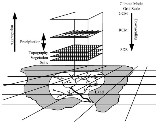
Figure 1.
Conceptual diagram of climate downscaling: converting global-scale model data into local-scale climate information. The figure shows aggregation and disaggregation processes across spatial scales. GCM (Global Climate Model), RCM (Regional Climate Model), and SDS (Statistical DownScaling) represent different levels of climate modeling and downscaling approaches. Inputs such as precipitation, topography, vegetation, and soils affect land surface processes at finer resolutions [14].

Table 1.
The key differences, advantages and disadvantages of SDSM and MACA models [23,24,25,26].
1.3. Research Gaps and Study Contribution
Although there has been progress in hydrological modeling and climate downscaling, few studies have focused on how climate change affects water resources in coastal forest ecosystems. Recent research highlights the need for local studies that consider both natural and human-related pressures, especially in vulnerable areas like coastal plains [27,28]. This study helps fill that gap by:
- Comparing the MACA and SDSM to find suitable climate projections for the CNF.
- Using the MIDAS approach to choose an accurate set of precipitation data.
- Applying the WaSSI model with refined climate inputs to simulate future water yield.
This research links climate projection tools with hydrological modeling to inform forest and water management. This approach can be applied in various regions, not just coastal forests.
2. Materials and Methods
In this study, we examined how climate change could affect water yield using climate downscaling techniques and hydrological modeling. Precipitation and temperature data were collected from trusted weather stations in the study area to analyze recent climate trends and their effects on water behavior. To simulate future climate conditions, two statistical downscaling methods were applied: the SDSM and MACA. These methods were chosen for their ability to generate detailed local climate data suitable for hydrological modeling [29,30]. The SDSM uses past weather data like rainfall and temperature to create detailed predictions of future climate conditions. To improve accuracy, the model was first adjusted (calibrated) using this real data and then applied to GCM scenarios to explore possible future changes in climate [31]. The SDSM also includes an ensemble approach for predicting precipitation, which means it produces several possible future outcomes to better reflect uncertainty in climate forecasts [32].
In this study, we applied the MIDAS approach to improve climate input data for hydrological modeling. This approach started with generating twenty precipitation ensembles using the SDSM to reflect future climate uncertainty. We then applied a range of statistical and machine learning techniques to evaluate these scenarios. The XGBoost algorithm performed best and was used to create a refined, composite precipitation series [33]. This step is central to the MIDAS approach, helping reduce uncertainty in climate inputs and supporting more accurate hydrological simulations.
The MACA model uses past climate patterns to create detailed future climate data. By working with gridded datasets, it can show how temperature and rainfall change across different areas, which makes it useful for studying local climate conditions [34]. Both the SDSM and MACA used the same GCM scenarios to ensure consistency in model comparison. We used several statistical metrics including mean, standard deviation, correlation coefficient, Mean Absolute Error (MAE), Root Mean Square Error (RMSE), and Correlation Coefficient (R2) to compare the predicted averages and variability in both precipitation and temperature. These measures allowed us to assess how well each model simulated past climate patterns and helped identify the more reliable method for generating future climate projections [35]. Temperature projections were generally more accurate across both models. This aligns with previous findings that precipitation is inherently more variable and difficult to downscale than temperature due to its spatial and temporal complexity [36]. Although both models performed well, the SDSM had an advantage because it could produce more detailed ensemble outputs, which helped better analyze uncertainty [37], whereas MACA delivered higher spatial resolution and better representation of climate extremes [38,39]. To assess how climate change could affect water yield, we used the WaSSI model [40], powered by the climate inputs generated through MIDAS. To address this, we generated 20 ensemble precipitation series using the SDSM and applied the MIDAS approach to select the most representative one for hydrological modeling.
Using WaSSI in the CNF showed that it works well for estimating water yield in areas with complex hydrology. Because it can adjust to different climate and land use conditions, it gave more reliable results than other models [41]. Also, recent studies comparing WaSSI with the InVEST model showed that WaSSI is more effective for estimating annual water yield, especially in coastal areas like the study region [22]. This approach combines advanced downscaling methods with the hydrological strengths of WaSSI to estimate future water yield under different climate scenarios. MIDAS plays a key role in refining precipitation inputs, while the focus remains on simulating and analyzing long-term water yield projections.
2.1. Study Area
The CNF is in eastern North Carolina, USA, and covers about 647 km2. It is a flat, low-lying area close to the Atlantic Ocean, surrounded by rivers like the Bogue Sound, White Oak River, and Neuse River (Figure 2).
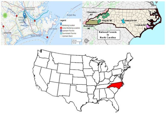
Figure 2.
Maps showing the study area. (Top left) Location of the Croatan National Forest (CNF) and hydrology monitoring stations. (Top right) Distribution of the four National Forests in North Carolina, including the CNF in the coastal region highlighted in pink. (Bottom) Location of North Carolina highlighted in red within the United States. River Bend is indicated by the green dot labeled with the number 2 [42].
These features create a mix of land and water ecosystems, including swamps, saltwater estuaries, and pine forests. The CNF features mostly sandy and poorly drained soils, which influence hydrological responses. Its vegetation includes longleaf pine and pocosin wetlands, with a growing season that typically extends from March through October. Because of its location and landscape, the forest is sensitive to climate-related changes such as sea-level rise, saltwater intrusion, and changing rainfall patterns. This makes it a suitable place to study how climate change can affect water yield. To help evaluate model performance, streamflow data from a nearby United States Geological Survey (USGS) gauge station (Brice Creek, Hydrologic Unit Code (HUC) 03020204) were used. This station was selected for its proximity and relevance to the study area, providing a reliable reference point for evaluating model performance. Due to its low elevation and proximity to coastal waters, the study area generally has a high-water table, which influences runoff, infiltration, and overall hydrological behavior.
2.2. Water Yield Model (WaSSI)
The WaSSI model is a useful tool for estimating water yield. Water yield refers to the amount of water that leaves a watershed after losses from soil storage, evapotranspiration, and land use are subtracted. It is usually measured in millimeters per year [43,44]. The WaSSI model, developed by the United States Department of Agriculture (USDA) Forest Service Southern Research Station, simulates water resources on both yearly and monthly scales. It includes advanced hydrological processes such as snow accumulation and melting, soil moisture tracking, evapotranspiration, and estimating runoff based on land cover types [45,46,47]. The model has been tested in many different climates and land uses, and it is known for being flexible and reliable when used to study how climate change may affect water yield [48,49]. WaSSI performed better than other models such as InVEST in estimating annual water yield, showing that it can be reliable for regions like the CNF [22]. The full details of the model, including the equations for evapotranspiration and runoff, were explained in our previous study [22]. In that study, the model was tested using historical data from the same area, and the results showed that it could simulate water balance components accurately. Therefore, in this study, the same validated WaSSI model is used to estimate future water yield using projected temperature and precipitation data under climate change scenarios. We use the WaSSI model with optimized monthly climate data from 2015 to 2060 to estimate annual water yield in the study area.
2.3. Statistical Downscaling Methods in Climate Data Analysis: SDSM and MACA
In recent years, climate downscaling methods have improved, mainly because we need more detailed climate data to understand local and regional impacts of climate change. Two well-known statistical downscaling methods, the SDSM and MACA, are widely used for this purpose and have become important tools in climate studies [50,51].
2.3.1. Statistical DownScaling Model (SDSM)
The SDSM is a widely used method that helps convert large-scale climate data into detailed local climate information. It builds statistical relationships between general atmospheric variables and observed local weather. The main steps include choosing key climate predictors, calibrating the model using past weather data, and then generating future climate data based on those relationships [31]. This approach is useful for creating more accurate local projections from coarse climate model outputs.
In the SDSM, daily precipitation is modeled in two sub-steps. In the first sub-step, a stochastic process determines whether precipitation occurs on a given day, which is modeled by the equation
where is the intercept, is the precipitation occurrence index for day , are the normalized predictor variables for day , are the regression coefficient, is the total number of predictors, and is the index of the predictors. Precipitation occurs on day if is less than or equal to a random number drawn from a uniform distribution between 0 and 1.
In the second sub-step, if precipitation occurs, the amount is estimated using a z-score regression model, given by
where is the intercept, is the z-score of precipitation for day , are regression coefficients, are the standardized predictors, is the index of the predictors, and is a normally distributed stochastic error term. The actual precipitation value is then calculated as
where is the standard normal cumulative distribution function, and is the inverse of the empirical Cumulative Distribution Function (CDF) of observed daily precipitation.
In the second step, daily temperature is simulated using a multiple linear regression model, expressed
where is the simulated temperature on day , is the intercept term, are the regression coefficients, are the standardized predictor variables for day , is the total number of predictors, is the index of the predictors, and is a normally distributed random error term.
After simulating daily precipitation and temperature with SDSM, its simplicity and efficiency became evident, making it suitable for regional climate studies [52,53,54]. In this study, the SDSM was used to generate localized climate data for the CNF. Twenty precipitation ensembles were produced to capture uncertainty, while a single temperature time series was used due to consistency across simulations.
Ensemble Selection Techniques
To identify the most representative precipitation time series among the 20 ensemble members generated by SDSM, several ensemble selection techniques were assessed. These methods differ in computational complexity, accuracy, and their ability to capture temporal variability and inter-member dependencies.
Best Single Member
This method selects the ensemble member with the lowest calibration error during the training phase. Although it is computationally efficient, it is sensitive to temporal anomalies and does not make use of the information contained in other ensemble members, which may reduce the reliability of the projections.
Weighted Average
This method gives each ensemble member a weight based on how well it performed in the past, then calculates a weighted average. It is better than just using one member because it uses all of them. However, it assumes that each member’s impact stays the same over time and cannot capture complex or changing relationships.
Multiple Linear Regression (MLR)
This method uses all ensemble members together in a linear regression model to make predictions. It usually gives better results than simpler methods because it uses more information. However, since it assumes relationships are linear and can struggle when the members are too similar, its accuracy may be limited in some cases.
Extreme Gradient Boosting (XGBoost)
XGBoost is a tree-based ensemble learning algorithm that builds additive regression trees in a stage-wise manner, optimizing a regularized objective function given by
where is the total objective function to be minimized, is loss function easuring the difference between true and predicted values (e.g., squared error), and is regularization term for -th tree, designed to prevent overfitting by penalizing complex trees.
where is regularization the penalty on the number of leaves in each tree, is the number of leaves (terminal nodes), is regularization coefficient that penalizes large leaf weights, and is the squared L2 norm of the vector of leaf weights (sum of squared leaf weights).
XGBoost is particularly suited for ensemble selection in climate applications due to its capability to handle missing values, multicollinearity, and nonlinear interactions among predictors. Furthermore, it automatically identifies the most informative features, balancing predictive accuracy with model simplicity [55].
2.3.2. Multivariate Adaptive Constructed Analogs (MACA)
In the MACA method, downscaling is performed by identifying historical analog days that closely resemble the large-scale climate patterns of a target future day. The downscaled value is computed as a weighted average of observed values from those analog days, using the equation
where is downscaled climate variable (e.g., temperature or precipitation) at future time t and location , are weights for each analog day based on its similarity to the GCM predictors at time , are climate variable from analog day , and is the number of analog days used. The weights are calculated based on the multivariate distance (e.g., Euclidean) between the predictor variables of the GCM for day t and those of historical days , and are normalized such that for each target day. This allows for improved temporal and spatial consistency in the downscaled projections. This method improves spatial and temporal accuracy in climate projections and is widely used in regional studies [56]. The next section shows the results, including climate predictions and their effects on water yield in the study area.
2.4. Time Scale of Data in the Modeling Process
Climate variables (precipitation and temperature) were spatially downscaled at a daily resolution using the SDSM and MACA models. However, since the WaSSI model requires monthly inputs and is sensitive to seasonal climate changes, these daily data were aggregated to a monthly scale. The selection and comparison of the downscaled climate data were performed at the monthly level to accurately capture seasonal hydroclimatic patterns. The WaSSI model was then run using these monthly inputs to simulate water yield at both monthly and annual scales. Although the model can produce outputs at finer resolutions, this study reports only annual results averaged over decades to emphasize long-term climate trends and minimize year-to-year variability. See Figure 3 for the modeling workflow.
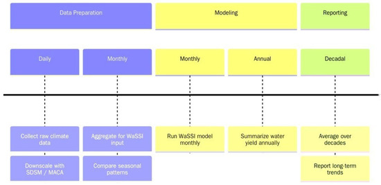
Figure 3.
Modeling framework: from daily climate data to decadal water yield using SDSM, MACA, and WaSSI.
2.5. Model Input Data
This study applied climate and hydrological modeling to assess future conditions in the Croatan National Forest (CNF), using two sources of climate data. MACAv2-METDATA offers ready-to-use, statistically downscaled CMIP5 projections for the Continental United States (CONUS) region, including the study area. In contrast, SDSM was used to downscale raw CMIP5 outputs from the CanESM2 model based on local observations. Since both sources rely on CMIP5 projections from CanESM2 under (RCPs) scenarios, the key difference lies in the downscaling methods used (Table 2).
Table 2.
Summary of climate datasets used for precipitation and temperature.
The WaSSI model was run using a variety of input data, including precipitation, temperature, land use, and soil characteristics. Table 3 lists the main data sources used for estimating water yield in the CNF.
Table 3.
Data sources for the WaSSI model.
3. Results
This section presents the key findings of the study in a structured manner. First, the outputs of two statistical downscaling approaches, the SDSM and MACA, are presented to provide localized climate projections. These projections include future trends in temperature and precipitation. Next, we apply the WaSSI hydrological model to simulate future water yield under various GCM scenarios. The results highlight differences in climate projections between downscaling methods and quantify the potential impacts of climate change on water availability in the study region.
3.1. Climate Downscaling Results
3.1.1. SDSM Projections of Temperature
The SDSM was calibrated using observed climate data from 1981 to 2014 to develop robust statistical relationships for temperature downscaling. Through iterative testing, specific humidity and 500 hPa geopotential height were identified as the most effective large-scale atmospheric predictors from the NCEP-DOE daily dataset. These variables consistently showed strong correlations with local temperature across all months. The calibration process yielded high model performance, with an average R2 of 0.75, and values exceeding 0.83 in certain months such as November and December. Additionally, Durbin–Watson statistics were consistently close to 2.0, indicating minimal autocorrelation in the residuals and confirming the statistical reliability of the model outputs [63]. Overall, the selected predictors and calibration results demonstrate that the SDSM can provide accurate and dependable localized temperature projections when properly configured. In the next step, to validate the model, temperature data for the period 2015–2022 were generated using the SDSM with predictors obtained from GCMs. The analysis of model performance during the calibration and validation periods indicates behavioral stability and satisfactory generalizability to independent datasets. As illustrated in Figure 4, during the calibration period (1981–2014), the distribution of monthly residuals was largely centered around zero, suggesting high model accuracy in reproducing temperature patterns, particularly in the summer season. Although greater variability in residuals is observed during the colder months, the overall trend remains consistent. A similar performance pattern is evident in the validation period (2015–2022), as shown in Figure 5, where the model successfully captures seasonal temperature fluctuations and maintains an acceptable level of predictive accuracy. The relative consistency of the model’s behavior across both periods confirms the coherence of the outputs and affirms the model’s reliability under varying temporal conditions. The final step involved generating future temperature projections for the period 2023–2060 using GCM-based predictors through the Scenario Generator module of SDSM.
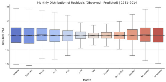
Figure 4.
Monthly Boxplots of Observed and Simulated Daily Temperatures during the Calibration Period (1981–2014), using NCEP-DOE predictors.
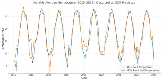
Figure 5.
Comparison of observed and GCM-based simulated monthly average temperatures during the validation period (2015–2022).
The temperature in the CNF has increased steadily from 1981 to 2022, and is projected to continue increasing to 2060, showing clear signs of climate warming. As shown in Figure 6, the average annual temperature rose by 0.121 °C per decade during 1981–2022 and is projected to rise faster 0.187 °C per decade between 2023 and 2060. Temperature variability also increased over time, with more extreme heat events and warm nights (Figure 6).
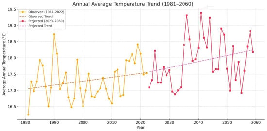
Figure 6.
Annual average temperature trends from observed (1981–2022, yellow) and projected (2023–2060, red) data using the SDSM. Dashed lines show warming trends with relevance to evapotranspiration and water yield.
Seasonal trends (Figure 7) show that all seasons are warming, especially summer and winter, which may increase evaporation and transpiration. Compared to the past, future temperatures are expected to be 0.60 °C higher (Figure 8) likely to reduce water yield.
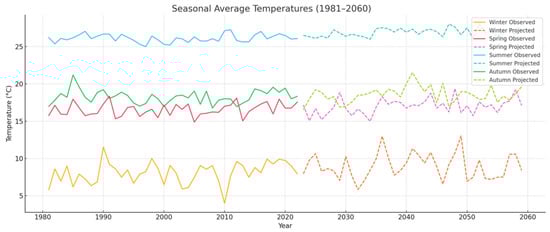
Figure 7.
Seasonal Temperature Trends (1981–2060).
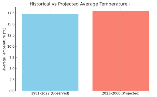
Figure 8.
Comparison of Historical and Projected Average Temperatures.
A major climate shift was detected around 2015 (Figure 9), marking the onset of a warmer, less stable period consistent with global temperature records that year [63]. Local observations also report more hot days, intense but less frequent rainfall, sea level rise causing ghost forests, and higher wildfire risk. In the next section, we compare the SDSM and MACA for temperature inputs in WaSSI.
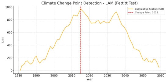
Figure 9.
Climate change point detection using the Pettitt test [64] applied to temperature data, showing a statistically significant change around 2015. The orange line represents the cumulative statistic , defined as the maximum absolute value of the rank-based cumulative sum of differences between two segments of the time series. The peak of , marked by the red dashed line, identifies the most probable change point, implying a shift to a new climatic phase relevant to evapotranspiration and water yield modeling.
SDSM vs. MACA for Temperature Inputs in WaSSI
Reliable projections of temperature and precipitation are important for estimating water yield with the WaSSI model and assessing potential impacts of climate change. In this section, the projected temperature results from two downscaling methods, MACA and SDSM, were compared. MACA outputs are readily available for the United States [60] and can be used to compare and evaluate the accuracy of the data produced by the SDSM. However, in many other regions of the world, MACA data is not readily available, and the method must be implemented separately.
In this section, the performance of these two statistical temperature prediction models was evaluated using observational data from 2015 to 2022. Based on the error metrics in Table 4, the SDSM had the lowest Mean Absolute Error (MAE = 1.80 °C), and Root Mean Square Error (RMSE = 2.56 °C), as well as a higher coefficient of determination (R2 = 0.866), showing better overall accuracy compared to MACA. The time-series trend (Figure 10) further confirms that the SDSM more accurately follows the seasonal patterns of observed temperatures.
Table 4.
Error Metrics of Temperature Prediction Models.
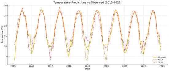
Figure 10.
Time-series comparison of observed temperatures versus MACA and SDSM predictions over the full period 2015 to 2022.
The scatter plots (Figure 11A, B) show that SDSM predictions align more closely with the ideal 1:1 line. Additionally, residual plots (Figure 12A, B) indicate that the SDSM has lower variance and less systematic bias. Therefore, both quantitative metrics and visual comparisons suggest that the SDSM is the more accurate and reliable compared to MACA, and its downscaled temperature data were used as inputs to the WaSSI model to assess future changes.
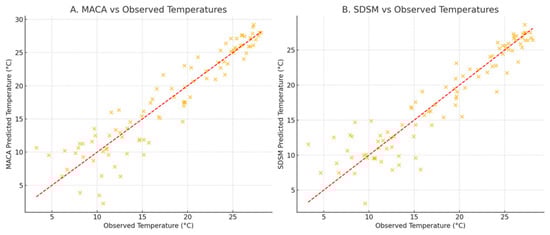
Figure 11.
(A,B) Comparison between observed temperatures and those predicted by MACA (A) and SDSM (B). Each orange cross (×) represents an individual observed–predicted temperature pair. The red dashed line indicates the 1:1 line, representing perfect agreement between observed and predicted values.
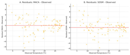
Figure 12.
(A,B) Residual plots for MACA (A) and SDSM (B), showing the difference between predicted and observed temperatures. Each orange cross (×) represents an individual residual value at a given observed temperature. The red dashed line indicates the zero-residual line.
In the next section, we will evaluate the calibration and validation of the precipitation projection using SDSM.
3.1.2. SDSM Projections of Precipitation
In this section, the SDSM was calibrated for the period 1981–2014 using two large-scale atmospheric variables from the NCEP-DOE dataset: the meridional wind component at 850 hPa (V850) and the geopotential height at 850 hPa (Z850). Daily precipitation data were paired with these predictors to train the model, resulting in an average R2 of 0.56. For validation, daily outputs from a GCM were used to generate 20 ensemble precipitation series for the period 2015–2022, to test the model’s ability to reproduce recent climate conditions. In the next step, to reduce precipitation prediction errors, the MIDAS approach was applied.
Improved Precipitation Simulation with MIDAS
Precipitation is one of the most challenging climate variables to simulate accurately due to its unstable behavior and high spatial variability. Statistical models like the SDSM have limitations in capturing these patterns. To address this, the MIDAS approach was applied, combining 20 ensembles of downscaled precipitation with the XGBoost algorithm to reduce prediction errors and improve model accuracy. To find the most accurate precipitation series from the 20 ensembles produced by the SDSM, we first tested simple methods like the Best Single Model and Weighted Average. However, these approaches had high monthly errors (MAE of 69.99% and 68.78%) and could not fully capture the complexity of precipitation. Next, we applied Multiple Linear Regression, which improved the results (MAE reduced to 39.42%) but was still limited in handling nonlinear patterns. Finally, we used machine learning techniques and found that the XGBoost algorithm performed best, lowering the MAE to 17.56%. Due to its high accuracy, XGBoost was selected as the core of the MIDAS approach. The results closely matched observed and prediction data, confirming the effectiveness of this method. Figure 13 shows the monthly comparison between observed precipitation and the predictions made by the XGBoost-based ensemble model as part of the MIDAS approach from 2015 to 2022. The results indicate that the model successfully captures the general patterns and seasonal variability of precipitation. Although some differences are noticeable during peak rainfall events, the overall agreement between observed and predicted values demonstrates the model’s reliability in reproducing monthly precipitation trends. The following examines precipitation changes in the CNF.
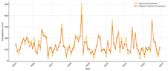
Figure 13.
Comparison of monthly precipitation: observed data vs. predictions from the XGBoost selected ensemble in the MIDAS approach (2015–2022).
Based on the long-term trends in observed (1981–2022) and predicted (2023–2060) precipitation, seasonal and monthly precipitation patterns (Figure 14) show a pronounced shift toward the warmer months in the predicted period. This redistribution has critical implications for the timing of runoff generation and groundwater recharge, both of which directly affect water yield. Additionally, the Standardized Precipitation Index (SPI), calculated over a 12-month scale (Figure 15), reveals considerable interannual variability, highlighting alternating periods of drought and wetness. These fluctuations underscore the increasing uncertainty in water yield projections under future climate conditions. The findings show that it is important to consider both long-term precipitation patterns and seasonal changes when planning water resources.
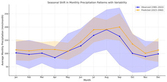
Figure 14.
Mean monthly precipitation for observed (1981–2022, blue) and projected (2023–2060, orange) periods, with shaded bands showing variability (±1 SD). The shift indicates increased summer and decreased winter rainfall, with key implications for future water yield modeling.
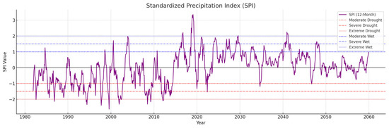
Figure 15.
Time series of the 12-month Standardized Precipitation Index (SPI) (1981–2060).
As shown in Figure 16, precipitation data shows clear changes in 2006, 2014, and 2016, suggesting shifts in climate patterns. This matches temperature results, which also show 2015 as a key year of climate change. These changes can directly affect water yield, so it is important to consider them in future assessments. This change in rainfall pattern may be partly influenced by the El Niño–Southern Oscillation (ENSO). Notably, 2010 and 2015 both marked as potential change points in the data coincided with strong ENSO phases (a strong La Niña in 2010 and a strong El Niño in 2015). Several studies have shown that ENSO events significantly affect rainfall and streamflow in the southeastern United States. These events can cause unusual seasonal rainfall patterns and increase climate variability in the region [65,66]. These findings suggest that ENSO related climate shifts may have played a role in the observed rainfall changes in this study area.
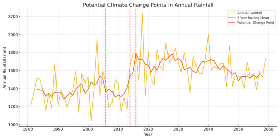
Figure 16.
Annual rainfall trends from 1980 to 2060, highlighting potential climate change points. The orange line represents annual rainfall, the bold red line shows the 5-year rolling mean, and the dashed vertical red lines indicate possible climate change points, suggesting sudden or gradual shifts in rainfall patterns.
Figure 17 shows a shift in annual rainfall patterns from 1981 to 2060, with 2015 marking a clear turning point. Before 2015, rainfall generally increased over time. After 2015, however, the trend begins to decline, with projections showing a gradual decrease through 2060. While some years still show high rainfall after 2015, the overall pattern suggests a long-term downward trend. This decline, along with increasing year-to-year variability, may signal a shift in the region’s climate. Such changes could reduce water availability, lower annual water yield, and affect the ecological balance in forested coastal areas.
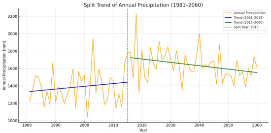
Figure 17.
Split trend analysis of annual precipitation from 1981 to 2060, highlighting 2015 as a climatic turning point. The orange line represents annual precipitation totals, while the blue and green lines indicate linear trends for the periods 1981–2015 and 2015–2060, respectively.
MIDAS-Integrated SDSM vs. MACA for Precipitation Inputs in WaSSI
To assess the accuracy of precipitation data for input into the WaSSI model, downscaled precipitation outputs from two models, MACA and a MIDAS-integrated SDSM, were compared against observed records from 2015 to 2022. MACA outputs are available for the United States and can be used to compare and evaluate the accuracy of the data produced by the SDSM [60].The evaluation included statistical metrics such as Mean Absolute Error (MAE), Root Mean Square Error (RMSE), the correlation coefficient, and the Nash–Sutcliffe Efficiency (NSE), as summarized in Table 5. The MIDAS-integrated SDSM consistently outperformed MACA, showing significantly lower errors, higher correlation, and a much better NSE value indicating closer agreement with observed data.
Table 5.
Statistical Comparison of Precipitation Downscaling: MACA vs. MIDAS-SDSM.
The time series comparison in Figure 18 shows that the MIDAS-SDSM follows the observed precipitation patterns more closely than MACA, which shows larger deviations. Similarly, the scatter plots in Figure 19A,B indicate that MIDAS-SDSM predictions are more tightly clustered around line 1:1. Monthly and seasonal error analyses (Figure 20 and Figure 21) also support these results, showing that the MIDAS-SDSM provides more accurate and consistent precipitation estimates throughout the year. Therefore, the MIDAS-SDSM downscaled precipitation data were used in the WaSSI model to estimate future water yield changes.
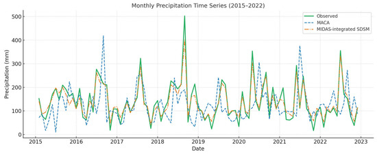
Figure 18.
Monthly precipitation (2015–2022): observed (green), MACA (blue dashed), and MIDAS-integrated SDSM (orange dash-dotted).
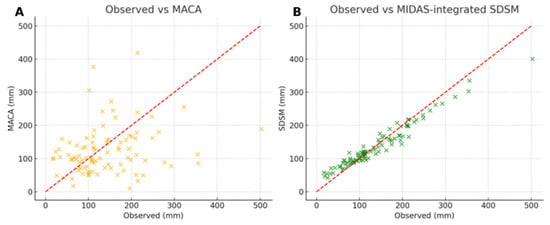
Figure 19.
(A,B) Scatter plots comparing observed precipitation with model-predicted values. (A) Comparison between observed data and the output of the MACA model; (B) Comparison between observed data and the output of the SDSM model integrated with MIDAS. Each × symbol represents a data pair consisting of an observed and predicted value. The red dashed line represents the 1:1 reference line.
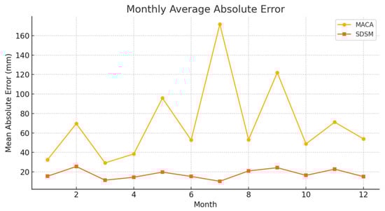
Figure 20.
Monthly average absolute error of precipitation predictions by MACA and MIDAS-integrated SDSM.
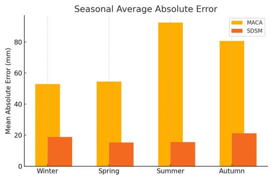
Figure 21.
Seasonal average absolute error for MACA and MIDAS-integrated SDSM across winter, spring, summer, and autumn.
3.2. Trends and Projections of Water Yield Using the WaSSI Model
Understanding how water availability might change under future climate conditions is essential, especially for sensitive ecosystems like the CNF, because water is a key part of natural resources and the environment. Changes in water supply can affect forest ecosystems, including vegetation dynamics, wildlife habitats, and groundwater systems. Knowing what might happen helps us protect nature and manage these areas more responsibly in the future [67,68].
In this study, we used the WaSSI hydrological model to estimate water yield from 1961 to 2060. For this purpose, as previously explained, the climate input data for the WaSSI model included temperature and precipitation from the historical period (1961–2022), obtained from the PRISM database [57]. Temperature data for the future period (2023–2060) were generated using the SDSM, and precipitation data for the same period were produced using the combined SDSM–MIDAS. For running the WaSSI model, in addition to climate data, Leaf Area Index (LAI) derived from MODIS imagery, land cover maps based on the 2006 NLCD, and watershed-level soil parameters from the STATSGO dataset were used (Table 3). Based on the results of trend analysis and climate variability, particularly the Pettitt test (Figure 9) and change points in annual precipitation (Figure 16), a significant climate shift appears to have occurred around the year 2015. This change is evident not only in the statistical structure of precipitation but also in the mean and increased variability. Considering this shift and its impact on rainfall, it is crucial to examine the projected water yield over the period 1961 to 2060. After 2015, more intense climate variability is expected to significantly affect the region’s hydrological behavior. Therefore, the year 2015 was selected as a baseline for comparison in water yield analysis, enabling a clearer evaluation of hydrological changes before and after this turning point. This temporal division helps us better understand and assess the potential effects of climate change on surface water resources and the ecosystems that depend on them. The analysis of Total Annual Water Yield (YLD) from 1961 to 2060 indicates that climate change has had a significant impact on both the quantity and variability of water production. As shown in Figure 22, the overall trend in annual water yield begins to decline steadily around 2015. This year is marked as a turning point for climate-related changes and is highlighted with a red dashed line.
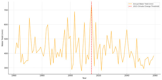
Figure 22.
Total Annual Water Yield (YLD) from 1961 to 2060, simulated using the WaSSI model. The red dashed line indicates the year 2015, which is marked as the threshold year for climate change.
Figure 23 presents a 10-Year Moving Average to smooth out annual fluctuations and reveal the long-term trend more clearly. The graph shows a continuous and gradual decline in YLD after 2015, which serves as a warning sign for the need to revise natural resource planning strategies.
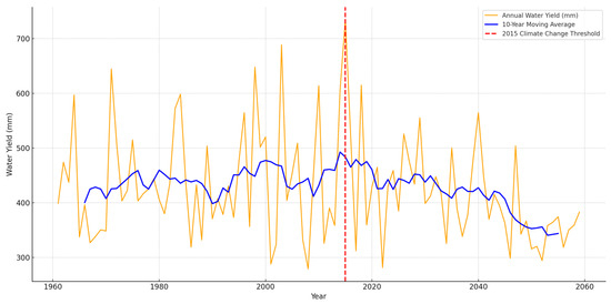
Figure 23.
Annual Water Yield (YLD) and 10-year moving average from 1961 to 2060, based on WaSSI model outputs. The red dashed line marks the 2015 climate change threshold.
Figure 24 displays the annual anomalies in water yield relative to the long-term average. Before 2015, most anomalies were positive, whereas most years after 2015 show negative deviations. This shift signals the onset of a period characterized by persistent declines in water production, likely due to decreased precipitation, increased evaporation, and disruptions in the region’s hydrological regime.
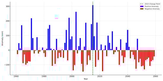
Figure 24.
Annual water yield anomalies (deviation from long-term mean) from 1961 to 2060. Positive and negative anomalies are shown in blue and red, respectively. The green dashed line marks the 2015 change point.
Figure 25 presents a comparative boxplot illustrating the statistical distribution of YLD before and after 2015. The post-2015 period shows a noticeable decrease in the median, a narrower Inter- Quartile Range (IQR), and lower maximum and minimum values. These changes point to a significant reduction in water yield and a heightened risk of drought and hydrological stress in the future.
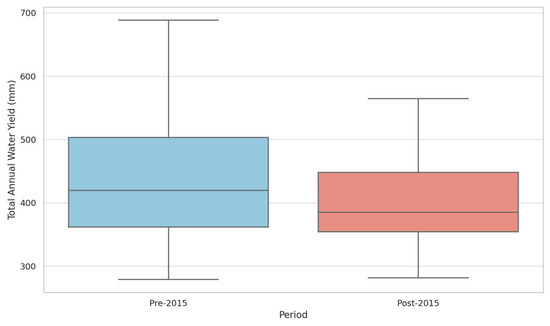
Figure 25.
Boxplot comparison of total annual water yield for pre-2015 and post-2015 periods. A noticeable decline in median and overall distribution is observed after 2015.
Water yield projections, derived from the integrated modeling steps, provide the basis for the following discussion.
4. Discussion
Accurate climate predictions are key to understanding how water resources might change in the future. In this study, we tested two statistical downscaling methods for estimating future precipitation and temperature. In comparison between the two downscaling methods, the SDSM showed better performance than MACA in simulating both temperature and, more notably, precipitation. Statistical indicators such as MAE, RMSE, correlation coefficient, and the NSE all indicated improved results for SDSM. Based on this, the SDSM was used to generate twenty ensemble precipitation series, which were then refined using the XGBoost machine learning algorithm. This integration, applied through the MIDAS approach, resulted in a noticeable reduction in prediction errors. The use of machine learning helped improve model accuracy by capturing nonlinear relationships among climate variables. Given that precipitation is often one of the more challenging variables to downscale, this combined approach helped reduce uncertainty and improve the reliability of the projections.
The temperature and precipitation projections indicate that the study area is experiencing notable climate change. This study examines the period 1981–2060. The historical analysis (1981–2022) shows a steady rise in mean annual temperature, and the projections for 2023–2060 indicate that this trend is likely to continue. The Pettitt test also points to a noticeable climate shift around 2015, associated with changes in temperature and precipitation patterns. These changes may gradually influence regional climate and water systems, especially in sensitive coastal ecosystems such as the CNF, in North Carolina. The year 2060 was selected only as the endpoint of this study. In future studies, the focus can be on extending projections up to the end of the 21st century to gain a broader understanding of long-term trends and a wider range of potential impacts of climate change.
The analysis of precipitation trends in the study area suggests a potential shift between the historical period (1981–2022) and the projected future period (2023–2060). While there was a modest upward trend in total annual precipitation in the past, future projections indicate a possible gradual decline in the coming decades. Changes in the seasonal distribution of precipitation are also evident, with peak precipitation expected to shift from spring and winter to summer and fall. This shift may increase the risk of seasonal floods and agricultural droughts. The year 2015 appears to mark a turning point in regional precipitation patterns, as the overall trend becomes downward afterward, despite occasional increases in certain months. This gradual decline, along with greater interannual variability, may reflect a transition toward a different climatic regime.
The Standardized Precipitation Index (SPI) also indicates an increase in the frequency and severity of drought events after 2015. This trend aligns with the identified climate regime shift in the same year. Annual rainfall data show notable changes in specific years, such as 2003, 2010, and 2015, which may be linked to shifts in atmospheric conditions and regional evaporation patterns.
Hydrological responses are clearly reflected in the model results. water yield (YLD), simulated using the WaSSI model based on historical (1961–2022) and projected (2023–2060) temperature and precipitation data, shows a gradual and relatively consistent decline after 2015. The chart indicates that before 2015, YLD reached approximately 650 mm in some years, while after 2015, it generally remained below 600 mm in most years. Moving average and boxplot analyses also confirm a reduction in both the mean and variability of YLD. These findings are consistent with national-scale studies suggesting that rising temperatures can reduce water availability even when precipitation increases, due to higher evapotranspiration, which limits the amount of rainfall contributing to total water yield. Overall, the period through 2060 provides a useful time frame for assessing the medium-term impacts of climate change on regional water resources. It should be noted that WaSSI does not simulate rainfall intensity or short-duration storm events directly. Nonetheless, the model accounts for general soil characteristics, including water holding capacity, which helps represent broader hydrological trends.
Previous research has reported similar patterns regarding the impacts of rising temperatures and precipitation on water availability. For instance, one study in Bulgaria found that warmer temperatures led to increased spring runoff but reduced summer flows [69]. In Ethiopia, even with increased rainfall, water availability did not improve due to higher evaporation rates driven by warmer conditions [70,71,72]. Similar findings have been reported in several other studies, particularly in forested and semi-humid regions, where warming was shown to reduce water yield even when precipitation increased suggesting that the negative effects of rising temperatures can offset the potential benefits of greater precipitation [38,73,74,75,76,77,78].
Although our study focused on the effects of climatic variables such as temperature and precipitation on water yield, national-scale modeling studies also support the notion that climate change exerts a more dominant influence on water yield variations than vegetation dynamics. For instance, projections using the MC2–WaSSI modeling framework—which combines the MAPSS-CENTURY version 2 (MC2) ecosystem model with the Water Supply Stress Index (WaSSI) hydrologic model have indicated substantial declines in water yield across many watersheds in the southeastern and central United States under climate change scenarios, particularly Representative Concentration Pathway (RCP) 8.5, a high-emissions scenario assuming continued increases in greenhouse gas concentrations without significant mitigation efforts. These declines are primarily attributed to shifts in temperature and precipitation, rather than vegetation characteristics such as leaf area index (LAI). These findings align with and indirectly support our results, underscoring the critical role of climatic drivers in shaping future water yield patterns. In line with recent recommendations advocating the use of more advanced climate projections climate projections within the MC2–WaSSI framework [50], our study incorporates downscaled data optimized through the SDSM–MIDAS approach to better capture future precipitation and temperature inputs and their impacts on hydrological processes.
What sets our study apart is its focus on coastal forested watersheds that are sensitive and hydrologically vulnerable like the CNF, which were not specifically examined in previous large-scale studies. Additionally, this study used high-resolution statistical downscaling to produce climate input data, improving the spatial accuracy and reliability of the results compared to relying only on global climate models [50,79,80].
This study may be useful for informing future research on climate impacts in similar coastal forested regions. The MIDAS approach, along with the SDSM, is fully generalizable and can be applied to any region or station where observed precipitation and temperature data are available. Future research could expand on this work by exploring a broader range of climate scenarios (e.g., various SSP pathways within CMIP6), applying the modeling framework to different ecological or climatic regions beyond the current study area, or integrating dynamic land use and land cover change projections to better assess their influence on water yield responses. Additionally, incorporating key socioeconomic factors such as population growth or land management decisions could improve the understanding of how human activities interact with climate to shape future hydrological outcomes. These insights may support adaptive and informed decision making in the face of future climate challenges.
5. Conclusions
This study examined climate change impacts in the CNF, North Carolina, and found that rising regional temperatures, shifts in the seasonal distribution of precipitation, and increased evapotranspiration have had a significant influence on water resources. Analysis of both historical data and future projections indicates that since 2015, the region has entered a new climate regime characterized by accelerated warming and reduced hydrological stability. The decline in both the magnitude and variability of annual water yield (YLD) after this transition reflects these changes clearly.
Comparison of downscaling approaches showed that the MIDAS approach combining statistical downscaling methods with machine learning produced more accurate simulations of precipitation than single method downscaling models. The use of updated climate scenarios and high-resolution input data further enhanced the spatial precision and reliability of projections. These findings align with other studies suggesting that in forested or humid regions, rising temperatures can reduce available water yield even when precipitation increases.
Overall, the results underscore the importance of understanding the complex interactions between climatic and hydrological variables for effective water resource planning. A focus on sensitive coastal ecosystems, supported by advanced modeling approaches, can provide a more suitable basis for developing climate-adaptive strategies. Future research that explores local-scale impacts and management responses could further support informed decision making in vulnerable regions.
Author Contributions
All research work, including conceptualization, methodology, formal analysis, investigation, data curation, original draft writing, visualization, and other research processes, was independently conducted by M.F. The remaining authors (S.A.C.N., P.C., J.P.R., S.B. and M.N.P.) contributed to writing (review and editing), supervision, resources, and administration. All authors have read and agreed to the published version of the manuscript.
Funding
This research received no external funding.
Data Availability Statement
The original contributions presented in this study are included in the article. For further information, please contact the corresponding author.
Acknowledgments
The authors declare that no external support or contributions were received in conducting this research.
Conflicts of Interest
The authors declare no conflicts of interest.
Disclaimer
Any opinions, findings, conclusions, or recommendations expressed in this material are those of the authors and do not necessarily reflect the views of the USDA. Any use of trade, firm, or product names is for descriptive purposes only and does not imply endorsement by the U.S. Government.
References
- Davis, M.B.; Shaw, R.G.; Etterson, J.R. Evolutionary responses to changing climate. Ecology 2015, 86, 1706–1714. [Google Scholar] [CrossRef]
- Bosch, J.M.; Hewlett, J.D. A review of catchment experiments to determine the effect of vegetation changes on water yield and evapotranspiration. J. Hydrol. 1982, 55, 3–23. [Google Scholar] [CrossRef]
- Sun, G.; Caldwell, P.; Noormets, A.; McNulty, S.G.; Cohen, E.; Myers, J.M.; Domec, J.-C.; Treasure, E.; Mu, Q.; Xiao, J.; et al. Upscaling key ecosystem functions across the conterminous United States by a watercentric ecosystem model. J. Geophys. Res. Biogeosci. 2011, 116, G00J05. [Google Scholar] [CrossRef]
- Zhang, L.; Cheng, L.; Chiew, F.; Fu, B. Understanding the impacts of climate and land use change on water yield. Adv. Water Resour. 2018, 33, 167–174. [Google Scholar]
- Nuñez, J.A.; Aguiar, S.; Jobbágy, E.G.; Jiménez, Y.G.; Baldassini, P. Climate change and land cover effects on water yield in a subtropical watershed spanning the Yungas–Chaco transition of Argentina. J. Environ. Manag. 2024, 358, 120808. [Google Scholar] [CrossRef]
- de Andrade Costa, D.; Bayissa, Y.; Villas-Boas, M.D.; Maskey, S.; Junior, J.L.; da Silva Neto, A.J.; Srinivasan, R. Water availability and extreme events under climate change scenarios in an experimental watershed of the Brazilian Atlantic Forest. Sci. Total Environ. 2024, 905, 167644. [Google Scholar]
- Ury, E.A.; Yang, X.; Wright, J.P.; Bernhardt, E.S. Rapid deforestation of a coastal landscape driven by sea-level rise and extreme events. Ecol. Appl. 2021, 31, e02339. [Google Scholar] [CrossRef]
- Bagstad, K.J.; Semmens, D.J.; Waage, S.; Winthrop, R. A comparative assessment of decision support tools for ecosystem services quantification and valuation. Ecosyst. Serv. 2013, 5, 27–39. [Google Scholar] [CrossRef]
- Garcia, X.; Estrada, L.; Saló, J.; Acuña, V. Blueing green water from forests as a strategy to cope with climate change in water-scarce regions: The case of the Catalan River basin district. J. Environ. Manag. 2024, 353, 120249. [Google Scholar] [CrossRef]
- Keller, A.A.; Garner, K.; Rao, N.; Knipping, E.; Thomas, J. Hydrological models for climate-based assessments at the watershed scale: A critical review of existing hydrologic and water quality models. Sci. Total Environ. 2023, 867, 161209. [Google Scholar] [CrossRef]
- Giorgi, F.; Mearns, L.O. Introduction to special section: Regional climate modeling revisited. J. Geophys. Res. Atmos. 1999, 104, 6335–6352. [Google Scholar] [CrossRef]
- Brekke, L.D.; Thrasher, B.L.; Maurer, E.P.; Pruitt, T. Downscaled CMIP3 and CMIP5 Climate Projections: Release of Downscaled CMIP5 Climate Projections, Comparison with Preceding Information, and Summary of User Needs; U.S. Department of the Interior, Bureau of Reclamation, Technical Services Center: Lakewood, CO, USA, 2013.
- Hessami, M.; Gachon, P.; Ouarda, T.B.M.J.; St-Hilaire, A. Automated regression-based statistical downscaling tool. Environ. Model. Softw. 2008, 23, 813–834. [Google Scholar] [CrossRef]
- Wilby, R.L.; Dawson, C.W. Using SDSM, Version 3.1. A decision support tool for the assessment of regional climate change impacts. Climate Change Unit, Environment Agency of England and Wales & Department of Computer Science, Loughborough University: Nottingham, UK, 2004.
- Abatzoglou, J.T.; Brown, T.J. A comparison of statistical downscaling methods suited for wildfire applications. Int. J. Climatol. 2012, 32, 772–780. [Google Scholar] [CrossRef]
- Wilby, R.L.; Dessai, S. Robust adaptation to climate change. Weather 2010, 65, 180–185. [Google Scholar] [CrossRef]
- Valencia, J.B.; Guryanov, V.V.; Mesa Diez, J.; Diaz, N.; Escobar Carbonari, D.; Gusarov, A.V. Predictive assessment of climate change impact on water yield in the Meta River Basin, Colombia: An InVEST model application. Hydrology 2024, 11, 25. [Google Scholar] [CrossRef]
- Rocha, J.; Quintela, A.; Serpa, D.; Keizer, J.J.; Fabres, S. Water yield and biomass production on a eucalypt-dominated Mediterranean catchment under different climate scenarios. J. For. Res. 2023, 34, 1263–1278. [Google Scholar] [CrossRef]
- Lockaby, G.; Nagy, C.; Vose, J.M.; Ford, C.R.; Sun, G.; McNulty, S.; Caldwell, P.; Cohen, E.; Moore Myers, J. Forests and water. In The Southern Forest Futures Project: Technical Report; Wear, D.N., Greis, J.G., Eds.; Gen. Tech. Rep. SRS-GTR-178; USDA Forest Service, Southern Research Station: Asheville, NC, USA, 2013; pp. 309–339. [Google Scholar]
- Caldwell, P.V.; Sun, G.; McNulty, S.G.; Cohen, E.C.; Moore Myers, J. Impacts of impervious cover, water withdrawals, and climate change on river flows in the conterminous US. Hydrol. Earth Syst. Sci. 2012, 16, 2839–2857. [Google Scholar] [CrossRef]
- Sun, S.; Sun, G.; Caldwell, P.; McNulty, S.; Cohen, E.; Xiao, J.; Zhang, Y. Drought impacts on ecosystem functions of the U.S. National Forests and Grasslands: Part I, evaluation of a water and carbon balance model. For. Ecol. Manag. 2015, 353, 260–268. [Google Scholar] [CrossRef]
- Fallahi, M.; Nelson, S.A.C.; Beyene, S.; Caldwell, P.V.; Roise, J.P. A comparative assessment of Water Supply Stress Index (WaSSI) and Integrated Valuation of Ecosystem Services and Tradeoffs (InVEST) models for annual water yield estimation: A case study in the Croatan National Forest. Environments 2025, 12, 89. [Google Scholar] [CrossRef]
- Kim, J.B.; Jiang, Y.; Hawkins, L.R.; Still, C.J. A comparison of multiple statistically downscaled climate change datasets for the conterminous USA. Environ. Res. Commun. 2022, 4, 125005. [Google Scholar] [CrossRef]
- Wang, G.; Kirchhoff, C.J.; Seth, A.; Abatzoglou, J.T.; Livneh, B.; Pierce, D.W.; Ding, T. Projected changes of precipitation characteristics depend on downscaling method and training data: MACA versus LOCA using the U.S. Northeast as an example. J. Hydrometeorol. 2020, 21, 2739–2758. [Google Scholar] [CrossRef]
- Keller, A.A.; Garner, K.L.; Rao, N.; Knipping, E.; Thomas, J. Downscaling approaches of climate change projections for watershed modeling: Review of theoretical and practical considerations. PLoS Water 2023, 2, e0000046. [Google Scholar] [CrossRef]
- Dorji, S.; Herath, S.; Mishra, B.K. Future climate of Colombo downscaled with SDSM-neural network. Climate 2017, 5, 24. [Google Scholar] [CrossRef]
- Sun, S.; Xiang, W.; Shuai, O.; Hu, Y.; Peng, C. Balancing water yield and water use efficiency between planted and natural forests: A global analysis. Glob. Change Biol. 2024, 30, e17561. [Google Scholar] [CrossRef] [PubMed]
- Farooqi, T.J.A.; Irfan, M.; Zhou, X.; Pan, S.; Atta, A.; Li, J. Advancing knowledge in forest water use efficiency under global climate change through scientometric analysis. Forests 2024, 15, 1893. [Google Scholar] [CrossRef]
- Gagnon, S.; Singh, B.; Rousselle, J.; Roy, L. An application of the Statistical DownScaling Model (SDSM) to simulate climatic data for streamflow modelling in Québec. Can. Water Resour. J. 2005, 30, 297–314. [Google Scholar] [CrossRef]
- Clark, S.; Mills, G.; Brown, T.; Harris, S.; Abatzoglou, J.T. Downscaled GCM climate projections of fire weather over Victoria, Australia. Part 1: Evaluation of the MACA technique. Int. J. Wildland Fire 2021, 30, 585–595. [Google Scholar] [CrossRef]
- Karamouz, M.; Nazif, S.; Falahi, M. Hydrology and Hydroclimatology: Principles and Applications; CRC Press: Boca Raton, FL, USA, 2013; Chapter 9; pp. 24–31. [Google Scholar]
- Zhina, D.; Avilés, A.; González, L.; Astudillo, A.; Astudillo, J.; Matovelle, C. Effects of Climate Change and Changes in Land Use and Cover on Water Yield in an Equatorial Andean Basin. Hydrology 2024, 11, 157. [Google Scholar] [CrossRef]
- Zhu, H.; Liu, H.; Zhou, Q.; Cui, A. A XGBoost-Based Downscaling-Calibration Scheme for Extreme Precipitation Events. IEEE Trans. Geosci. Remote Sens. 2023, 61, 4103512. [Google Scholar] [CrossRef]
- Heidari, A.; Watkins, D.; Mayer, A.; Propato, T.; Verón, S.; Abelleyra, D. Spatially variable hydrologic impact and biomass production tradeoffs associated with Eucalyptus (E. grandis) cultivation for biofuel production in Entre Rios, Argentina. GCB Bioenergy 2021, 13, 823–837. [Google Scholar] [CrossRef]
- Villamizar, S.R.; Pineda, S.M.; Carrillo, G.A. The effects of land use and climate change on the water yield of a watershed in Colombia. Water 2019, 11, 285. [Google Scholar] [CrossRef]
- Tebaldi, C.; Sansó, B. Joint projections of temperature and precipitation change from multiple climate models: A hierarchical Bayesian approach. J. R. Stat. Soc. Ser. A Stat. Soc. 2009, 172, 83–106. [Google Scholar] [CrossRef]
- Maraun, D.; Wetterhall, F.; Ireson, A.M.; Chandler, R.E.; Kendon, E.J.; Widmann, M.; Brienen, S.; Rust, H.W.; Sauter, T.; Themeßl, M.; et al. Precipitation downscaling under climate change: Recent developments to bridge the gap between dynamical models and the end user. Rev. Geophys. 2010, 48, RG3003. [Google Scholar] [CrossRef]
- González-Rojí, S.; Wilby, R.; Sáenz, J.; Ibarra-Berastegi, G. Harmonized evaluation of daily precipitation downscaled using SDSM and WRF+WRFDA models over the Iberian Peninsula. Clim. Dyn. 2019, 53, 1413–1433. [Google Scholar] [CrossRef]
- Eum, H.I.; Cannon, A.J.; Murdock, T.Q. Intercomparison of multiple statistical downscaling methods: Multi-criteria model selection for South Korea. Stoch. Environ. Res. Risk Assess. 2017, 31, 683–703. [Google Scholar] [CrossRef]
- Sun, G.; McNulty, S.G.; Moore Myers, J.A.; Cohen, E.C. Impacts of multiple stresses on water demand and supply across the southeastern United States. J. Am. Water Resour. Assoc. 2008, 44, 1441–1457. [Google Scholar] [CrossRef]
- Bagstad, K.J.; Cohen, E.; Ancona, Z.H.; McNulty, S.G.; Sun, G. The sensitivity of ecosystem service models to choices of input data and spatial resolution. Appl. Geogr. 2018, 93, 25–36. [Google Scholar] [CrossRef]
- U.S. Forest Service. Schedule of Proposed Actions (SOPA)—North Carolina [Map]. U.S. Department of Agriculture, Forest Service. Available online: https://www.fs.usda.gov/sopa/state-level.php?nc (accessed on 10 August 2025).
- Zhao, Z.Y.; Fu, B.J.; Lu, Y.H.; Li, T.; Deng, L.; Wang, Y.L.; Lu, D.; Wang, Y.; Wu, X. Variable climatic conditions dominate decreased wetland vulnerability on the Qinghai-Tibet Plateau: Insights from the ecosystem pattern-process-function framework. J. Clean. Prod. 2024, 458, 142496. [Google Scholar] [CrossRef]
- Sun, G.; McNulty, S.G.; Lu, J.; Amatya, D.M.; Liang, Y.; Kolka, R.K. Regional annual water yield from forest lands and its response to potential deforestation across the southeastern United States. J. Hydrol. 2005, 308, 258–268. [Google Scholar] [CrossRef]
- Caldwell, P.V.; Miniat, C.F.; Elliott, K.J.; Swank, W.T.; Brantley, S.T.; Laseter, S.H. Declining water yield from forested mountain watersheds in response to climate change and forest mesophication. Glob. Change Biol. 2016, 22, 2997–3012. [Google Scholar] [CrossRef]
- Werner, C.; Meredith, L.K.; Ladd, S.N.; Ingrisch, J.; Kübert, A.; van Haren, J.; Bahn, M.; Bailey, K.; Bamberger, I.; Beyer, M.; et al. Ecosystem fluxes during drought and recovery in an experimental forest. Science 2021, 374, 1514–1518. [Google Scholar] [CrossRef]
- Liu, N.; Shaikh, M.A.; Kala, J.; Harper, R.J.; Dell, B.; Liu, S.; Sun, G. Parallelization of a distributed ecohydrological model. Environ. Model. Softw. 2018, 101, 51–63. [Google Scholar] [CrossRef]
- Sun, S.; Sun, G.; Cohen, E.; McNulty, S.G.; Caldwell, P.V.; Duan, K.; Zhang, Y. Projecting water yield and ecosystem productivity across the United States by linking an ecohydrological model to WRF dynamically downscaled climate data. Hydrol. Earth Syst. Sci. 2016, 20, 935–952. [Google Scholar] [CrossRef]
- Liu, N.; Dobbs, G.R.; Caldwell, P.V.; Miniat, C.F.; Sun, G.; Duan, K.; Nelson, S.A.C.; Bolstad, P.V.; Carlson, C.P. Inter-Basin Transfers Extend the Benefits of Water from Forests to Population Centers Across the Conterminous U.S. Water Resour. Res. 2022, 58, e2022WR032051. [Google Scholar] [CrossRef]
- Duarte, H.F.; Kim, J.B.; Sun, G.; McNulty, S.G.; Xiao, J. Climate and vegetation change impacts on future conterminous United States water yield. J. Hydrol. 2024, 639, 131472. [Google Scholar] [CrossRef]
- Tang, J.; Niu, X.; Wang, S.; Gao, H.; Wang, X.; Wu, J. Statistical downscaling and dynamical downscaling of regional climate in China: Present climate evaluations and future climate projections. Adv. Atmos. Sci. 2016, 33, 632–646. [Google Scholar] [CrossRef]
- Dafouf, S.; Lahrach, A.; Tabyaoui, H.; Benaabidate, L. Future Evolutions of Precipitation and Temperature Using the Statistical DownScaling Model (SDSM), Case of the Guir and the Ziz Watershed, Morocco. Earth 2025, 6, 4. [Google Scholar] [CrossRef]
- Wilby, R.L.; Hay, L.E.; Leavesley, G.H. A comparison of downscaled and raw GCM output: Implications for climate change scenarios in the San Juan River basin, Colorado. J. Hydrol. 1999, 225, 67–91. [Google Scholar] [CrossRef]
- Karamouz, M.; Fallahi, M.; Nazif, S.; Rahimi Farahani, M. Long lead rainfall prediction using statistical downscaling and artificial neural network modeling. Sci. Iran. Trans. A Civ. Eng. 2009, 16, 165–172. [Google Scholar]
- Chen, T.; Guestrin, C. XGBoost: A scalable tree boosting system. In Proceedings of the 22nd ACM SIGKDD International Conference on Knowledge Discovery and Data Mining, San Francisco, CA, USA, 13–17 August 2016; ACM: New York, NY, USA, 2016; pp. 785–794. [Google Scholar]
- Shukla, R.; Khare, D.; Dwivedi, A.K.; Rudra, R.P.; Palmate, S.S.; Ojha, C.S.P.; Singh, V.P. Evaluation of statistical downscaling model’s performance in projecting future climate change scenarios. J. Water Clim. Change 2023, 14, 3559–3595. [Google Scholar] [CrossRef]
- PRISM Climate Group. PRISM Climate Data. Oregon State University. Available online: https://prism.oregonstate.edu/ (accessed on 31 May 2024).
- NOAA Physical Sciences Laboratory. NCEP/DOE Reanalysis 2 Data. Available online: https://psl.noaa.gov/data/gridded/data.ncep.reanalysis2.html (accessed on 31 May 2024).
- Government of Canada. Climate Model Projections: CanESM2. Canadian Climate Data and Scenarios. Available online: https://climate-scenarios.canada.ca/?page=pred-canesm2 (accessed on 31 May 2024).
- University of Idaho, MACA Team. Multivariate Adaptive Constructed Analogs (MACA) Downscaled Climate Data [Data set]. Available online: https://climate.northwestknowledge.net/MACA/ (accessed on 31 May 2024).
- NASA. MODIS Leaf Area Index (LAI) and Fraction of Photosynthetically Active Radiation (FPAR) Product (MOD15A2H), Version 6.1 [Data Set]. NASA LP DAAC. Available online: https://www.earthdata.nasa.gov/data/catalog/lpcloud-mod15a2h-061 (accessed on 25 June 2023). [CrossRef]
- United States Department of Agriculture (USDA). Available online: https://www.usda.gov (accessed on 26 June 2023).
- Shen, X.; Luo, X.; Sang, X. A geographically weighted Durbin model for spatial downscaling of land surface temperatures. In Proceedings of the International Conference on Remote Sensing, Surveying, and Mapping (RSSM 2023), Changsha, China, 6–8 January 2023; SPIE: Bellingham, WA, USA, 2023; Volume 12710, p. 127100R. [Google Scholar]
- Pettitt, A.N. A non-parametric approach to the change-point problem. J. R. Stat. Soc. Ser. C (Appl. Stat.) 1979, 28, 126–135. [Google Scholar] [CrossRef]
- Zhang, C.; Li, S.; Luo, F.; Huang, Z. The global warming hiatus has faded away: An analysis of 2014–2016 global surface air temperatures. Int. J. Climatol. 2019, 39, 2116–2130. [Google Scholar] [CrossRef]
- Clark, C.; Nnaji, G.A.; Huang, W. Effects of El-Niño and La-Niña Sea surface temperature anomalies on annual precipitations and streamflow discharges in southeastern United States. J. Coast. Res. Spec. Issue 2014, 68, 113–120. [Google Scholar] [CrossRef]
- Li, S.; Agathokleous, E.; Li, S.; Xu, Y.; Xia, J.; Feng, Z. Climate gradient and leaf carbon investment influence the effects of climate change on water use efficiency of forests: A meta-analysis. Plant Cell Environ. 2023, 47, 1070–1083. [Google Scholar] [CrossRef] [PubMed]
- Liang, C.; Zhang, M.; Wang, Z.; Xiang, X.; Gong, H.; Wang, K.; Liu, H. The strengthened impact of water availability at interannual and decadal time scales on vegetation GPP. Glob. Change Biol. 2024, 30, e17138. [Google Scholar] [CrossRef]
- Chang, H.; Knight, C.; Staneva, M.P.; Kostov, D. Water resource impacts of climate change in southwestern Bulgaria. GeoJournal 2002, 57, 159–168. [Google Scholar] [CrossRef]
- Belihu, M.; Abate, B.; Tekleab, S.; Bewket, W. Hydro-meteorological trends in the Gidabo catchment of the Rift Valley Lakes Basin of Ethiopia. Phys. Chem. Earth Parts A/B/C 2018, 104, 84–101. [Google Scholar] [CrossRef]
- Lemann, T.; Roth, V.; Zeleke, G. Impact of precipitation and temperature changes on hydrological responses of small-scale catchments in the Ethiopian Highlands. Hydrol. Sci. J. 2017, 62, 270–282. [Google Scholar] [CrossRef]
- Wakjira, M.T.; Peleg, N.; Six, J.; Molnar, P. Green water availability and water-limited crop yields under a changing climate in Ethiopia. Hydrol. Earth Syst. Sci. 2025, 29, 863–886. [Google Scholar] [CrossRef]
- Udall, B.; Overpeck, J. The twenty-first century Colorado River hot drought and implications for the future. Water Resour. Res. 2017, 53, 2404–2418. [Google Scholar] [CrossRef]
- Lu, J.; Sun, G.; McNulty, S.G.; Amatya, D.M. Modeling actual evapotranspiration from forested watersheds across the southeastern United States. J. Am. Water Resour. Assoc. 2003, 39, 887–896. [Google Scholar] [CrossRef]
- Zhu, J.; Sun, G.; Li, W.; Zhang, Y.; Miao, G.; Noormets, A.; McNulty, S.G.; King, J.S.; Kumar, M.; Wang, X. Modeling the potential impacts of climate change on the water table level of selected forested wetlands in the southeastern United States. Hydrol. Earth Syst. Sci. 2017, 21, 6289–6305. [Google Scholar] [CrossRef]
- McLaughlin, D.L.; Kaplan, D.A.; Cohen, M.J. Managing forests for increased regional water yield in the southeastern U.S. Coastal Plain. J. Am. Water Resour. Assoc. 2013, 49, 953–965. [Google Scholar] [CrossRef]
- Ahmed, M.A.A.; Abd-Elrahman, A.; Escobedo, F.J.; Cropper, W.P., Jr.; Martin, T.A.; Timilsina, N. Spatially explicit modeling of multi-scale drivers of aboveground forest biomass and water yield in watersheds of the Southeastern United States. J. Environ. Manag. 2017, 199, 158–171. [Google Scholar] [CrossRef]
- Younger, S.E.; Jackson, C.R.; Rasmussen, T.C. Relationships among forest type, watershed characteristics, and watershed ET in rural basins of the Southeastern US. J. Hydrol. 2020, 591, 125316. [Google Scholar] [CrossRef]
- Shiogama, H.; Fujimori, S.; Hasegawa, T.; Hayashi, M.; Hirabayashi, Y.; Ogura, T.; Iizumi, T.; Takahashi, K.; Takemura, T. Important distinctiveness of SSP3–7.0 for use in impact assessments. Nat. Clim. Change 2023, 13, 1276–1278. [Google Scholar] [CrossRef]
- Inglis, N.C.; Brown, T.R.; Cale, A.B.; Hartsook, T.; Matos, A.; Onyegbula, J.; Greenberg, J. Quantifying spatially explicit uncertainty in empirically downscaled climate data. Int. J. Climatol. 2024, 44, 4548–4570. [Google Scholar] [CrossRef]


Disclaimer/Publisher’s Note: The statements, opinions and data contained in all publications are solely those of the individual author(s) and contributor(s) and not of MDPI and/or the editor(s). MDPI and/or the editor(s) disclaim responsibility for any injury to people or property resulting from any ideas, methods, instructions or products referred to in the content. |
© 2025 by the authors. Licensee MDPI, Basel, Switzerland. This article is an open access article distributed under the terms and conditions of the Creative Commons Attribution (CC BY) license (https://creativecommons.org/licenses/by/4.0/).