Article

GIANN—A Methodology for Optimizing Competitiveness Performance Assessment Models for Small and Medium-Sized Enterprises

by
Jones Luís Schaefer
1,*,
Paulo Roberto Tardio
2,
Ismael Cristofer Baierle
3 and
Elpidio Oscar Benitez Nara
2
1
Department of Production Engineering, Federal University of Santa Maria (UFSM), Santa Maria 97105-900, Brazil
2
Production and Systems Engineering Graduate Program, Pontifical Catholic University of Parana (PUCPR), Curitiba 80215-901, Brazil
3
Graduate Program in Agro-Industrial Systems and Processes, Federal University of Rio Grande, Rio Grande 96203-900, Brazil
*
Author to whom correspondence should be addressed.
Adm. Sci. 2023, 13(2), 56; https://doi.org/10.3390/admsci13020056
Submission received: 29 December 2022 / Revised: 6 February 2023 / Accepted: 9 February 2023 / Published: 10 February 2023

Abstract

:
The adoption of models based on key performance indicators to diagnose and evaluate the competitiveness of companies has been presented as a trend in the operations’ management. These models are structured with different variables in complex interrelationships, making diagnosis and monitoring difficult due to the number of variables involved, which is one of the main management challenges of Small and Medium-sized Enterprises. In this sense, this article proposes the Gain Information Artificial Neural Network (GIANN) method. GIANN is a method to optimize the number of variables of assessment models for the competitiveness and operational performance of Small and Medium-sized Enterprises. GIANN is a hybrid methodology combining Multi-attribute Utility Theory with Entropy and Information Gain concepts and computational modeling through Multilayer Perceptron Artificial Neural Network. The model used in this article integrates variables such as fundamental points of view, critical success factors, and key performance indicators. GIANN was validated through a survey of managers of Small and Medium-sized Enterprises in Southern Brazil. The initial model was adjusted, reducing the number of key performance indicators by 39% while maintaining the accuracy of the results of the competitiveness measurement. With GIANN, the number of variables to be monitored decreases considerably, facilitating the management of Small and Medium-sized Enterprises.

1. Introduction

Competitiveness is a broad term that combines managers’ concerns related to market share, profitability, outputs, exports, and employment levels (Carbone and Rivers 2020). Furthermore, the competitiveness and innovation of companies directly depend on improvements in their productivity, quality (Liu et al. 2022; Bhat et al. 2021), and the formation of dynamic and entrepreneurial environments (Baierle et al. 2021). These concerns heavily impact SMEs that form the backbone of development in most nations (Soni et al. 2022). The main challenges are industrial transformation and developing a high-quality production style (Villa and Taurino 2018). However, SMEs cannot identify the causes of these difficulties and challenges due to the lack of management control systems and difficulties measuring management performance (Kim et al. 2021), demonstrating the need for SMEs to have optimized and simplified models for diagnosing and measuring competitiveness.
The rapid industrial and technological development has increased competitiveness among companies, which have sought to establish strategies such as monitoring competitiveness through management metrics (Rodrigues et al. 2021) to improve decision-making (Baierle et al. 2019). The companies’ competitive performance must be measured to verify if the objectives are being reached (Kim et al. 2021). Therefore, this measurement becomes a basic requirement to effectively improve the competitiveness of companies (Yadav et al. 2020). In this sense, to measure competitiveness and assist in the decision-making process, Key Performance Indicators (KPIs) can be used as a set of metrics to manage and seek continuous improvement and effectiveness in productivity, quality, operational performance, and efficiency of an enterprise (Kang et al. 2016; Chytilova et al. 2019). KPIs must be defined based on business strategy, allowing organizations to translate abstract performance objectives into concrete, measurable metrics (Gilsing et al. 2021). There is no consensus among the authors regarding the number of KPIs to be used; Kaplan and Norton (1996) recommend less than 20 KPIs, while Hope and Fraser (2013) recommend less than 10. Thus, one must discern the appropriate number of KPIs to be used; often, many KPIs can end up generalizing specific problems. In contrast, a very small number may not effectively present the perceived reality of an enterprise.
In addition to KPIs, other metrics such as Critical Success Factors (CSFs) and Fundamental Points of View (FPVs) can be used to diagnose and assess companies’ competitiveness, bringing a qualitative-quantitative view to the model used. In this sense, CSFs are those areas where a company needs to achieve positive results to achieve its goals (Gupta et al. 2018; Rockart 1982) being used as a basis for adapting and improving company actions and processes (Swarnakar et al. 2020). These CSFs can compose models of diagnosis and measurement of competitive performance together with other variables, such as FPVs (Schaefer et al. 2022). The FPVs are those aspects considered fundamental to evaluate the possible actions to be taken, defining what is important in the decision-making context and what actions must be taken (e Costa et al. 1999) to ensure efficient and effective management of companies (Schaefer et al. 2021). Thus, FPVs make up the main group of variables in companies’ decision-making models (Ishizaka and Nemery 2013), enabling a direct assessment of companies’ business objectives. Therefore, the relevance of structuring models for diagnosing and measuring the competitiveness of companies is perceived. These models can encompass KPIs, CSFs, and FPVs in a multilevel structure (Silva Júnior et al. 2022). It is necessary to define which and how many these KPIs, CSFs, and FPVs will be, as well as how to integrate them into a competitiveness measurement model (Rodrigues et al. 2021).
The models for measuring the competitive performance of companies can be structured with the help of Multicriteria Decision Making (MCDM) methods. MCDM methods are commonly used to classify options and alternatives and solve problems where a decision needs to be made, such as choosing the best option, eliminating alternatives, and identifying or creating new strategies (Santos et al. 2022). To find a solution in a decision-making process, hierarchizing the variables in a decision tree format is a crucial step (Laforest et al. 2013), thus making it possible to carry out the intended diagnoses and evaluations. To solve this decision tree, an MCDM approach like Multi-attribute Utility Theory (MAUT) can be used. MAUT uses subjective decision-making judgments given by managers and experts to establish preferences about different consequences (da Silva et al. 2022). The results of applying the MCDM methods to models for measuring and evaluating competitiveness may differ depending on the method chosen, and to overcome this difficulty, hybridization with other methodologies is an option that should be considered. (Aktaş and Demirel 2021). Therefore, allying an MCDM technique, such as MAUT, with mathematical and computational techniques to aid the management and decision-making process can be successfully performed.
Based on these initial considerations, it can be said that SMEs are naturally concerned with monitoring and measuring their competitive and market performance. Managers of these companies should seek to develop simple and optimized models to measure the competitiveness of these companies, enabling easier management and being in line with what is required at the market level. The use of metrics, such as KPIs, associated with decision-making methodologies can become an important tool to monitor and measure the competitive performance of SMEs. In addition, structuring this tool by adding a methodology to optimize this modeling could further facilitate the management process of these companies.
Thus, this research aims to present the GIANN method. GIANN can be used to optimize and adjust the number of variables present in assessment models and frameworks that evaluate competitiveness in SMEs. To validate and show how GIANN can be applied, a case study was developed with SMEs from the South of Brazil. The companies’ competitiveness rates were calculated using the MAUT method based on an evaluation model that integrates variables such as FPVs, CSFs, and KPIs. The correlation between the KPIs and the competitive rates and the tests to optimize the initial evaluation model were operationalized through the Artificial Neural Network (ANN) Multilayer Perceptron (MLP), keeping the variation of the values of the competitiveness rates within limits previously defined as acceptable. Thus, GIANN can reduce the number of KPIs, CSFs, and FPVs, keeping the correlation coefficient between KPIs and competitiveness rates above a predetermined level.
The main contribution of this article is that, through GIANN, the number of variables to evaluate the competitiveness of the companies can be optimized and adjusted, demanding the monitoring and control of a smaller number of KPIs to accompany the evaluation of the companies’ competitiveness. It can also be highlighted that GIANN combines the multicriteria analysis method MAUT with mathematical techniques, such as entropy and information gain, and computational modeling through ANN MLP. From the SME’s point of view, it can be highlighted that the article presents a proposal for the assessment of competitiveness with a direction of which variables are more critical and unstable in companies of this size.
The remainder of the paper is organized as follows: Section 2 details the GIANN Method, Section 3 shows a case study, Section 4 presents the discussion and managerial implications, and Section 5 presents the conclusion of this paper.

2. GIANN Method

The GIANN method is subdivided into eight stages, as seen in Figure 1. Each one of these stages is detailed in the sequence.

2.1. Stage 1—Integration of KPIs, CSfs, and FPVs

The initial model for evaluating the competitiveness of SMEs used in this research is the one proposed by (Schaefer et al. 2020), which uses interdependent and correlated concepts such as FPVs, CSFs, and KPIs, integrating and hierarchizing them in a decision tree format. This decision tree makes it possible to calculate replacement rates using the MAUT method, thus measuring the SMEs’ competitiveness. Table 1 presents this initial model.
Figure 2 presents KPIs, CSFs, and FPVs in a decision tree format diagram. This diagram represents the initial variable integration used in this case study.

2.2. Stage 2—Data Collection

The second stage of the proposed methodology consists of surveying to collect data with specialists in the research area. The case study of this article was developed from a survey sent by e-mail to 67 managers of industry SMEs linked to productive extension programs of the Secretary of Economic Development Science and Technology of Rio Grande do Sul, Brazil. The survey questions to SME managers used a 5-point Likert Scale (1 = not important until 5 = extremely important). In these questions, SME managers pointed out the level of importance that each of the 18 KPIs of the competitive performance measurement model to effectively assess these companies’ competitiveness rate.

2.3. Stage 3—Calculation of Competitiveness Rates Using the MAUT Method

MAUT (Fishburn 1970; Keeney and Raiffa 1976) has one of the best theoretical bases for applications involving risk and uncertainty since it not only deals with the choice of an alternative but also allows analyzing the decision (Monte and de Almeida-Filho 2016). The MAUT allows the establishment of an evaluation scale of alternatives (Aktaş and Demirel 2021); from this, the utility values for each alternative are calculated (Ozkaya et al. 2021). The ease of combining with other optimization methods in the search for an optimal solution (Wu et al. 2012) was the reason why this method was chosen for this research.
The MAUT method allows the proposition of decision models with more variables, and replacement rates are used to carry out the transition of calculations from one level to another. The replacement rates demonstrate the differences in importance between each criterion of the modeling, allowing them to be evaluated quantitatively (de Almeida 2013). They can be obtained by ordering the evaluation criteria and then constructing the semantic matrix of the value judgment in the same scale used for the value function (Ensslin et al. 2000). In the case study, to calculate the ICRs of SMEs, it is necessary to calculate the local replacement rates of KPIs, CSFs, and FPVs, allowing for assessing the competitiveness perception of SME managers at each level of the proposed model according to Equation (1) (KPIs), Equation (2) (CSFs), and Equation (3) (FPVs) initially proposed in Schaefer et al. (Schaefer et al. 2020).
L R R K P I = K P I k
where:
  • LRRKPI: KPI local replacement rate;
  • KPI: the value of KPI responses;
  • k: number of KPIs within the CSF.
L R R C S F = 1 n L R R K P I   k w
where:
  • LRRCSF: CSF local replacement rate;
  • n: number of KPIs of the CSF;
  • LRRKPI: KPIs’ local replacement rate;
  • k: number of KPIs within the CSF;
  • w: number of KPIs within the FPV.
L R R F P V = 1 n L R R C S F   w x
where:
  • LRRFPV: FPV local replacement rate;
  • n: number of CSFs within the FPV;
  • LRRCSF: CSF local replacement rate;
  • w: number of KPIs within the FPV;
  • x: total number of KPIs.
FPVs’ local replacement rates allow for calculating the SMEs’ ICRs (Equation (4)).
I C R = 1 n L R R F P V
where:
  • ICR: individual competitiveness rate;
  • LRRFPV: FPV local replacement rate;
  • n: number of FPVs.
The ICR values provide a view of the perception of managers about the SMEs’ competitiveness which takes into account the variables presented in the evaluation model initially proposed in Table 1 and Figure 2. This article aims to propose a methodology that allows for optimizing these competitiveness assessment models, reducing the number of variables to be monitored by managers, and keeping the results of the competitiveness assessment similar to the initial model. For this, the GIANN method proposes using the information gain each KPI brings to the model.

2.4. Stage 4—Calculation of KPIs Information Gain

To obtain the information gain that each KPI brings to the modeling, it is necessary to calculate the entropy of the system, which is a measure of how uncertain the content of information is in a random variable (Bermudez-Edo et al. 2018). The maximum entropy principle determines the least informative probability distribution for a random variable given previous information about itself (Mendes et al. 2016). The calculation of the entropy is given by Equation (5):
E ( S ) = i 1 n p i l o g 2 ( p i )
where:
  • E(S): general network entropy;
  • n: number of elements;
  • p: the probability of occurrence of the element p.
With entropy, it is possible to calculate the information gain that each KPI brings to the model (Equation (6)). The information gain is calculated for each attribute (KPI), and the attribute with the highest information gain is designated as the root node (Kumar Pal and Pal 2013). In this research, we used the Weka software (WEKA 2022) to calculate the entropy and information gain each KPI provides to the initial competitiveness assessment model.
G ( S , A ) = E ( S ) V a l u e s   ( A ) | S v | | S | E ( S v )
where:
  • G(S, A): attribute A information gain as a function of the set S;
  • E(S): general network entropy;
  • Sv: number of occurrences of the element p in attribute A;
  • S: total number of occurrences in attribute A;
  • E(Sv): individual element entropy.
From the values of the information gains, it becomes possible to carry out the correlation tests of the model, removing the KPIs one by one and verifying if the values of the competitiveness rates remain above the desired values. The methodology proposed in this article uses the ANN for these tests.

2.5. Stage 5—Test Correlation by ANNs

ANN is a computational model based on biological neural networks which use multiple simple processors interconnected to learn the relationships between sets of variables (Hemmat Esfe et al. 2022). There are different types of ANNs, and the MLP network was chosen because it is a classification tree with at least three nodes: input, hidden, and output (Li et al. 2022), and each node of a layer has a connection to all nodes of the next layer through adaptive synaptic weights (Sarkar et al. 2019). This configuration partially approximates the initial measurement model presented in Figure 2. A backpropagation ANN was used to dynamically predict competitiveness rates, considering the uncertainties of the model (Lu et al. 2022) and predicting new data from supervised learning based on existing data. The mechanism used in learning functions as a sequential process iterative where information feed-forward, error calculation, error backpropagation, and weight adjustment occur (Kwon et al. 2018; Wong and Chan 2015). This process is repeated until the output error value converges to a minimum value.
Weka software (WEKA 2022) was used in this research to model the ANN. Modeling through Weka results in the weights and bias for each node, and a sigmoidal function is used for activation. Still, in cases where the data behaves linearly, the values of “S” provided by Weka must be considered linearly according to Equation (8). To obtain the general equation of the network, it is necessary to use Equations (7) and (8). Figure 3 graphically shows where the weights and bias influence the network, which is a simplified ANN with four inputs (×1, ×2, ×3, and ×4), a hidden layer with two nodes (S1 and S2), and one output (ICR):
I C R = W 0 + 1 n W n · S n
where:
  • ICR: Individual competitiveness rate obtained by ANN;
  • W0: Linear Node 0—Bias node 0;
  • W: Linear Node—Node synaptic weight;
  • S: Sigmoid Node—S function result.
For each node in the ANN hidden layers, it must calculate the value of S, which is the result of the linear function described by S (Equation (8)):
S = w 0 + 1 n w n · x n
where:
  • S: Node sigmoid—linear function result;
  • w0: Node 1 sigmoid—Node 1 bias;
  • wn: Node n sigmoid—Attribute xn synaptic weight;
  • xn: x values (KPIs).
To obtain the correlation between KPIs and ICRs, it was necessary to provide the values of the ICRs calculated using the MAUT method. These parameters must be provided to the MLP ANN so that it is trained (Fetene et al. 2018). The dataset obtained through the survey can be considered small to be applied to the ANN. However, with a smaller dataset, the network can be trained with a high level of performance, set with a learning rate of 0.01 and momentum of 0.01, allowing the tests to be performed quickly. The cross-validation mode was applied to optimize the available data set and to train ANN once it divides the dataset into training and validation objects. It is used when the dataset is too small to be divided into training and validation datasets (Xu et al. 2018). The input attributes for the ANN were the responses of the SME managers to the survey KPIs. We obtained the correlation coefficients between the KPIs and the competitiveness rates (ICRs) as output.

2.6. Stage 6—Withdraw the KPI with Less Information Gain

With the KPIs ranked according to the information gains, the exclusion tests can be carried out, starting with the exclusion of the ones with less information gain towards the ones with greater information gain. Thus, the network was tested again for each excluded KPI to verify the new correlation coefficient. The stopping point of the tests was when the pre-established correlation coefficient was reached. Pearson’s correlation coefficient measures the linear dependency between two random variables, where 0.9 indicates a very strong correlation (Ly et al. 2018). Wu et al. (2018) say that above 0.7 the Pearson Correlation coefficient is already considered satisfactory. Thus, for this research, it was proposed a correlation coefficient of 0.950. In this case study, the KPIs were removed until only one was left, and the correlation coefficient was calculated for demonstration.

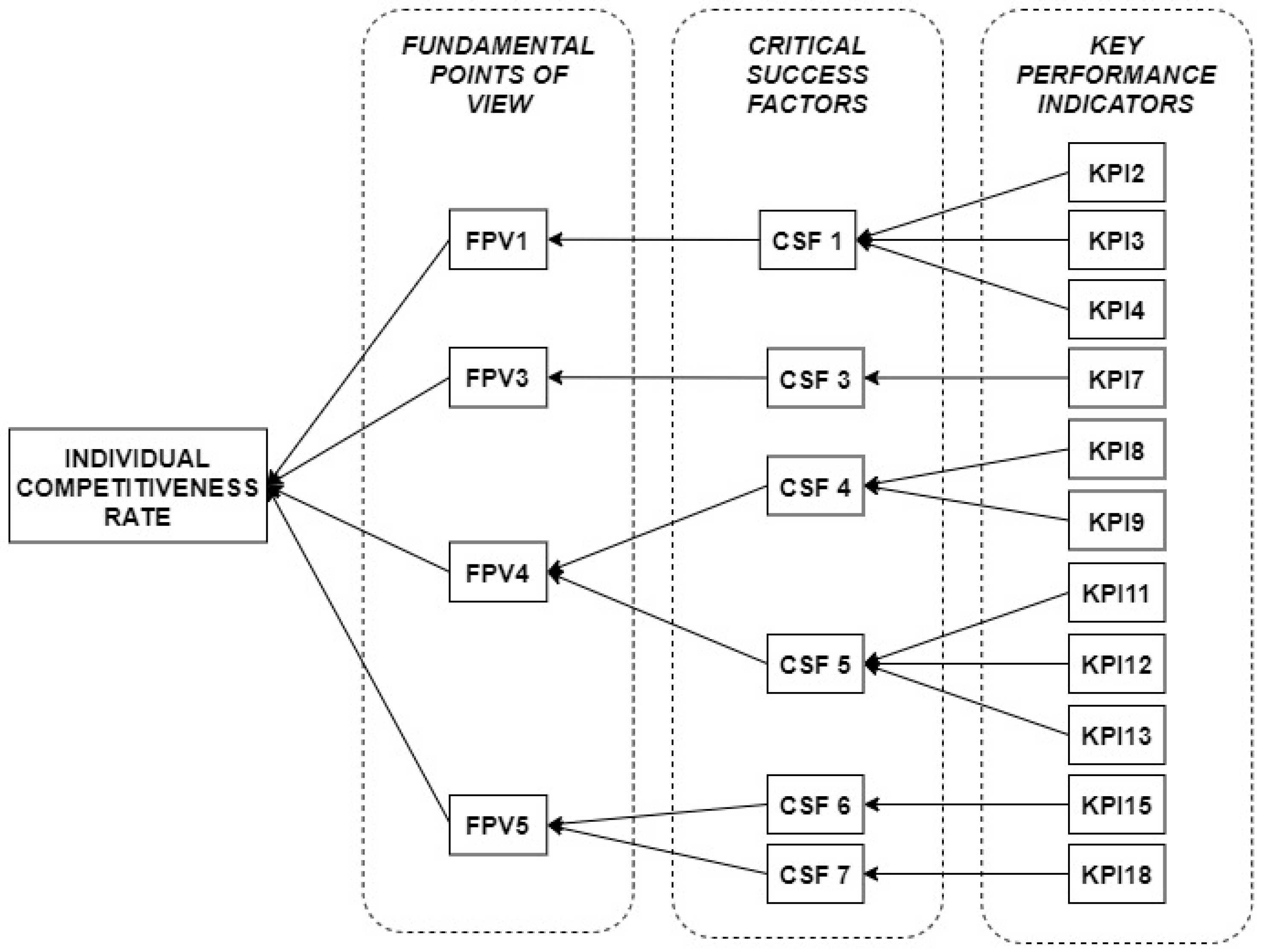
2.7. Stage 7—New Integration of KPIs, CSFs, and FPVs

Once the correlation coefficient was reached, a new hierarchy in a decision tree format was structured with the remaining KPIs, CSFs, and FPVs, giving rise to an optimized model for diagnosing and measuring the SMEs’ competitiveness.

2.8. Stage 8—Calculation of the New ICRs by MAUT

Finally, the new ICRs from the optimized model were calculated by the MAUT method using Equations (1)–(4).

3. Case Study with Small and Medium-Sized Enterprises

The initial model for diagnosing and measuring competitiveness was presented in Figure 1, consisting of 18 KPIs, 7 CSFs, 5 FPVs, and the ICR as output.

3.1. KPIs’ Information Gain Ranking

To make it possible to carry out tests that reduce the number of KPIs needed for the model and establish an order for removing KPIs, a ranking was generated (Table 2) with the average information gain each KPI brings to the model.

3.2. Correlation Tests by ANN

To perform the ANN tests, Weka automatically generated the model in Figure 4. This model, represented by the ANN shown in this figure, uses 18 KPIs as inputs, a hidden layer with nine nodes, and the ICR as the output. It is worth mentioning that, in the MAUT method, each KPI influences only one CSF, and each CSF influences only one FPV, while in the ANN, each KPI influences all nodes of the hidden layer, distributing the weights among these nodes. By applying the results of the competitiveness rates obtained by the MAUT method as parameters for the ANN, it was possible to obtain the correlation coefficient between the KPIs and these rates and the absolute and quadratic errors, both provided by Weka.
The GIANN method, after stage 5, has a decision point where it is checked whether the correlation coefficient is satisfactory. In this paper, for correlation to be considered satisfactory, it should be above 0.950. However, as a way of exemplifying, we presented in Figure 5 the tests until there was only one KPI in the model. This way, we made the tests by removing KPI by KPI, starting with the last one placed in the ranking (KPI10), followed by KPI14, and successively until there was only one KPI in the model (KPI11). Figure 5 is a graph with the progression of the correlation coefficients and the absolute and quadratic errors according to the KPI reduction tests.
In this paper, the remaining KPIs’ correlation coefficient is defined as equal to or greater than 0.950 regarding the initial ICR. The optimization proposed for the competitiveness assessment model was to exclude 7 KPIs with the lowest information gain. In this proposal, the correlation coefficient reached was 0.9501, and the absolute error was 0.0969. The following KPIs were excluded: 10, 14, 16, 17, 5, 6, and 1. It is possible to perceive a good performance of the proposal due to the following factors: the reduction in the number of KPIs maintains the correlation between the variables and a level of error low; and the fact that the KPIs that were excluded have little variability, bringing little information to the model.

3.3. New Integration of KPIs, CSFs, and FPVs

At this stage of the GIANN method, a new integration between KPIs, CSFs, and FPVs is performed, generating an optimized competitiveness measurement model. This new model is structured considering the decrease in the number of KPIs of the competitiveness measurement model from 18 to 11 and maintaining a correlation between the KPIs and the companies’ competitiveness rates at 0.9501. With the decrease in KPIs, CSF2 and FPV2 could also be excluded. Figure 6 shows the optimized model for measuring the competitiveness of SMEs.

3.4. New Competitiveness Rates by MAUT

With the optimized model to measure the competitiveness of SMEs, the new ICRs were calculated by the MAUT method. Table 3 presents the first results of SMEs’ ICR and the new SMEs’ ICR calculated by MAUT (the SMEs are coded by the letter E followed by numbers, and the ICR scale is the same as the survey, from 1 to 5).
The variation between the values obtained for the ICRs and the new ICRs was between 0.101 (+2.27%) for more, up to 0.525 (−14.4%) for less, with a medium variation of 0.173 (4.42%). A slight tendency for a decrease in the ICR values of the SMEs could be observed.
Remembering that the scale of the ICRs ranges from 1 to 5, E9 had the highest positive variation, ranging from 4.444 to 4.545, and E69 had the greatest negative variation, ranging from 3.889 to 3.364. The variation of the ICRs’ mean, called Global Competitiveness Rate (GCR), is shown in Table 4.
Another observation that can be made is that 10 SMEs occupy the same position in the two rankings, and another 10 had their positions changed only one position, more or less. This little variation can be considered positive given the large number of variables involved in the model, thus bringing safety to the GIANN method.

4. Discussion and Managerial Implications

The model optimization by the GIANN method reduced the number of KPIs to be monitored and controlled by order of 39% (from 18 KPIs to 11 KPIs) and has a direct impact on the SMEs management, which, considering their financial and technological limitations, may measure and control their competitiveness by making use of a smaller number of metrics, facilitating their managerial decision-making processes. Given the low variability between initial and optimized competitiveness rates, it can also be understood that KPIs that can be excluded do not need to be monitored and controlled to maintain the enterprise’s competitiveness because the desired level of efficiency will be maintained given the high correlation obtained between the variables and the competitiveness rates.
The ranking of the SMEs was performed to demonstrate that applying the GIANN method to optimize the competitiveness measurement model reduced the number of necessary KPIs, CSFs, and FPVs, and did not substantially modify the positions obtained by the SMEs. The initial model, which had 18 KPIs, 7 CSFs, and 5 FPVs, was optimized, resulting in an optimized model, maintaining a correlation coefficient above 0.950 and, therefore, a satisfactory mathematical accuracy. The optimized model consists of 11 KPIs, 6 CSFs, and 4 FPVs. GIANN enabled a 39% reduction in the number of KPIs in the model while maintaining a 95,01% correlation between the KPIs and the calculated competitiveness rates, demonstrating the reliability of the proposed method. GIANN method reduces the number of variables in such competitiveness measurement models, and it can be applied to other situations, exemplifying how the model can be simplified to aid decision-making while maintaining satisfactory results.

5. Conclusions

This article presented the GIANN method, a methodology used to optimize and adjust the number of variables present in models for measuring and evaluating the competitiveness of companies. The article focused on demonstrating an application of the proposed methodology in a case study with SMEs from the industry in southern Brazil. The management variables that served as the basis of the competitiveness measurement model presented were the KPIs, CSFs, and FPVs, which, after being ranked, were modeled to diagnose and assess the competitiveness of SMEs.
GIANN uses the MAUT multicriteria method, the concepts of entropy and information gain, and the ANN MLP in a hybrid way to evaluate and optimize models to measure the competitiveness of companies such as SMEs. Previously, the MONNA method was proposed to verify the quality of modeling to measure competitiveness (Baierle et al. 2020), de Moraes et al. (2019) used the Naive Bayes algorithm to simulate the probabilities of trade associations getting more members, and Immawan et al. (2019) proposed a KPI-based model to measure the performance of SMEs related to customers. In this sense, it is clear that the GIANN method, in addition to allowing the measurement of competitiveness, also allows optimizing the measurement model.
About the GIANN method, it can be said that the methodology streamlines and simplifies the monitoring and controlling variables such as KPIs. The application of the method defines a minimum set of variables that can satisfy the management needs of companies. With GIANN, KPIs that have little influence on business results are identified and do not need to be monitored regularly. Assuming that it is a fact with negative repercussions and greater variability in the KPIs, knowing how to select which these indicators are of paramount importance for good management of companies. In addition, a company can reapply the method when the set of controlled indicators no longer varies greatly. At this point, the company can reapply the method to verify if any indicator controlled in its management model can be replaced by another showing greater information gain.
This article had limitations regarding the level of specificity of the metrics and variables used, once in this article, three variables were used to measure the competitiveness of SMEs: KPIs, CSFs, and FPVs. However, in other applications, these variables may receive other nomenclatures and be applied to measure other objectives, such as innovation capacity. The number of model levels can be changed if the equations are suitable. It is suggested that, in the future, the GIANN method be applied to optimize the use of variables in applied models such as innovation in SMEs or the use of technology in SMEs.

Author Contributions

Conceptualization, J.L.S. and E.O.B.N.; methodology, J.L.S. and I.C.B.; investigation, J.L.S. and I.C.B.; resources, J.L.S. and E.O.B.N.; data curation, J.L.S. and I.C.B.; writing—original draft preparation, J.L.S., I.C.B. and P.R.T.; writing—review and editing, J.L.S., P.R.T. and E.O.B.N.; visualization, I.C.B. and E.O.B.N.; supervision, E.O.B.N.; project administration, E.O.B.N. All authors have read and agreed to the published version of the manuscript.

Funding

This research received no external funding.

Institutional Review Board Statement

Not applicable.

Informed Consent Statement

Not applicable.

Data Availability Statement

Data will be made available on request.

Conflicts of Interest

The authors declare no conflict of interest.

References

  1. Aktaş, Nadine, and Neslihan Demirel. 2021. A Hybrid Framework for Evaluating Corporate Sustainability Using Multi-Criteria Decision Making. Environment, Development and Sustainability 23: 15591–618. [Google Scholar] [CrossRef]
  2. Baierle, Ismael Cristofer, Jones Luis Schaefer, Miguel Afonso Sellitto, Leandro Pinto Fava, João Carlos Furtado, and Elpidio Oscar Benitez Nara. 2020. MOONA Software for Survey Classification and Evaluation of Criteria to Support Decision-Making for Properties Portfolio. International Journal of Strategic Property Management 24: 226–36. [Google Scholar] [CrossRef]
  3. Baierle, Ismael Cristofer, Julio Cezar Mairesse Siluk, Vinicius Jaques Gerhardt, Cláudia De Freitas Michelin, Álvaro Luiz Neuenfeldt, and Elpidio Oscar Benitez Nara. 2021. Worldwide Innovation and Technology Environments: Research and Future Trends Involving Open Innovation. Journal of Open Innovation: Technology, Market, and Complexity 7: 229. [Google Scholar] [CrossRef]
  4. Baierle, Ismael Cristofer, Miguel Afonso Sellitto, Rejane Frozza, Jones Luís Schaefer, and Anderson Felipe Habekost. 2019. An Artificial Intelligence and Knowledge-Based System to Support the Decision-Making Process in Sales. South African Journal of Industrial Engineering 30: 17–25. [Google Scholar] [CrossRef]
  5. Bermudez-Edo, Maria, Payam Barnaghi, and Klaus Moessner. 2018. Analysing Real World Data Streams with Spatio-Temporal Correlations: Entropy vs. Pearson Correlation. Automation in Construction 88: 87–100. [Google Scholar] [CrossRef]
  6. Bhat, Shreeranga, E. V. Gijo, Anil Melwyn Rego, and Vinayambika S. Bhat. 2021. Lean Six Sigma Competitiveness for Micro, Small and Medium Enterprises (MSME): An Action Research in the Indian Context. TQM Journal 33: 379–406. [Google Scholar] [CrossRef]
  7. Carbone, Jared C., and Nicholas Rivers. 2020. The Impacts of Unilateral Climate Policy on Competitiveness: Evidence from Computable General Equilibrium Models. Review of Environmental Economics and Policy 11: 24–42. [Google Scholar] [CrossRef]
  8. Chytilova, Ekaterina, Siyka Demirova, and Marie Jurova. 2019. Key Performance Indicators the Providers of Logistic Services: Experience of Selected Companies. Paper presented at 2019 II International Conference on High Technology for Sustainable Development (HiTech), Sofia, Bulgaria, October 10–11. [Google Scholar]
  9. de Almeida, Adiel Teixeira. 2013. Processo de Decisão Nas Organizações. São Paulo: Atlas. [Google Scholar]
  10. de Moraes, Jaqueline, Jones Luís Schaefer, Jacques Nelson Corleta Schreiber, Johanna Dreher Thomas, and Elpidio Oscar Benitez Nara. 2019. Algorithm Applied: Attracting MSEs to Business Associations. Journal of Business and Industrial Marketing 35: 13–22. [Google Scholar] [CrossRef]
  11. e Costa, Carlos A. Bana, Leonardo Ensslin, Émerson C. Cornêa, and Jean-Claude Vansnick. 1999. Decision Support Systems in Action: Integrated Application in a Multicriteria Decision Aid Process. European Journal of Operational Research 113: 315–35. [Google Scholar] [CrossRef]
  12. Ensslin, Leonardo, Ademar Dutra, and Sandra R. Ensslin. 2000. MCDA: A Constructivist Approach to the Management of Human Resources at a Governmental Agency. International Transactions in Operational Research 7: 79–100. [Google Scholar] [CrossRef]
  13. Fetene, Besufekad N., Rajkumar Shufen, and Uday S. Dixit. 2018. FEM-Based Neural Network Modeling of Laser-Assisted Bending. Neural Computing and Applications 29: 69–82. [Google Scholar] [CrossRef]
  14. Fishburn, Peter C. 1970. Utility Theory for Decision Making. McLean: Research Analysis Corp. [Google Scholar]
  15. Gilsing, Rick, Anna Wilbik, Paul Grefen, Oktay Turetken, Baris Ozkan, Onat Ege Adali, and Frank Berkers. 2021. Defining Business Model Key Performance Indicators Using Intentional Linguistic Summaries. Software and Systems Modeling 20: 965–96. [Google Scholar] [CrossRef]
  16. Gupta, Shivam, Subhas C. Misra, Ned Kock, and David Roubaud. 2018. Organizational, Technological and Extrinsic Factors in the Implementation of Cloud ERP in SMEs. Journal of Organizational Change Management 31: 83–102. [Google Scholar] [CrossRef]
  17. Hemmat Esfe, Mohammad, Sayyid Majid Motallebi, and Davood Toghraie. 2022. Investigation the Effects of Different Nanoparticles on Density and Specific Heat: Prediction Using MLP Artificial Neural Network and Response Surface Methodology. Colloids and Surfaces A: Physicochemical and Engineering Aspects 645: 128808. [Google Scholar] [CrossRef]
  18. Hope, Jeremy, and Robin Fraser. 2013. Beyond Budgeting: How Managers Can Break Free from the Annual Performance Trap. Boston: Harvard Business Press. [Google Scholar]
  19. Immawan, Taufiq, Annisa Indah Pratiwi, and Winda Nur Cahyo. 2019. The Proposed Dashboard Model for Measuring Performance of Small-Medium Enterprises (SME). International Journal of Integrated Engineering 11: 167–73. [Google Scholar] [CrossRef]
  20. Ishizaka, Alessio, and Philippe Nemery. 2013. Multi-Criteria Decision Analysis: Methods and Software. Hoboken: John Wiley & Sons. [Google Scholar]
  21. Kang, Ningxuan, Cong Zhao, Jingshan Li, and John A. Horst. 2016. A Hierarchical Structure of Key Performance Indicators for Operation Management and Continuous Improvement in Production Systems. International Journal of Production Research 54: 6333–50. [Google Scholar] [CrossRef]
  22. Kaplan, Robert S., and David P. Norton. 1996. The Balanced Scorecard: Translating Strategy into Action. Boston: Harvard Business Press. [Google Scholar]
  23. Keeney, R. L., and H. Raiffa. 1976. Decisions with Multiple Objectives: Preferences and Value Tradeoffs. Cambridge: Cambridge University Press. [Google Scholar]
  24. Kim, Doyeong, Wongyun Oh, Jiyeong Yun, Jongyoung Youn, Sunglok Do, and Donghoon Lee. 2021. Development of Key Performance Indicators for Measuring the Management Performance of Small Construction Firms in Korea. Sustainability 13: 6166. [Google Scholar] [CrossRef]
  25. Kumar Pal, Ajay, and Saurabh Pal. 2013. International Journal of Computer Science and Mobile Computing Evaluation of Teacher’s Performance: A Data Mining Approach. International Journal of Computer Science and Mobile Computing 2: 359–69. [Google Scholar]
  26. Kwon, He Boong, Jooh Lee, and Kristyn N. White Davis. 2018. Neural Network Modeling for a Two-Stage Production Process with Versatile Variables: Predictive Analysis for above-Average Performance. Expert Systems with Applications 100: 120–30. [Google Scholar] [CrossRef]
  27. Laforest, Valérie, Gaëlle Raymond, and É. Piatyszek. 2013. Choosing Cleaner and Safer Production Practices through a Multi-Criteria Approach. Journal of Cleaner Production 47: 490–503. [Google Scholar] [CrossRef]
  28. Li, Pengpeng, Jiping Liu, An Luo, Yong Wang, Jun Zhu, and Shenghua Xu. 2022. Deep Learning Method for Chinese Multisource Point of Interest Matching. Computers, Environment and Urban Systems 96: 101821. [Google Scholar] [CrossRef]
  29. Liu, Zheming, Saixing Zeng, Daxin Sun, and Chi Ming Tam. 2022. How Does Transport Infrastructure Shape Industrial Competitiveness? A Perspective from Industry Dynamics. IEEE Transactions on Engineering Management 69: 1378–93. [Google Scholar] [CrossRef]
  30. Lu, Renzhi, Ruichang Bai, Zhe Luo, Junhui Jiang, Mingyang Sun, and Hai Tao Zhang. 2022. Deep Reinforcement Learning-Based Demand Response for Smart Facilities Energy Management. IEEE Transactions on Industrial Electronics 69: 8554–65. [Google Scholar] [CrossRef]
  31. Ly, Alexander, Maarten Marsman, and Eric Jan Wagenmakers. 2018. Analytic Posteriors for Pearson’s Correlation Coefficient. Statistica Neerlandica 72: 4–13. [Google Scholar] [CrossRef]
  32. Mendes, R. R. A., A. P. Paiva, R. S. Peruchi, P. P. Balestrassi, R. C. Leme, and M. B. Silva. 2016. Multiobjective Portfolio Optimization of ARMA–GARCH Time Series Based on Experimental Designs. Computers & Operations Research 66: 434–44. [Google Scholar] [CrossRef]
  33. Monte, Madson B.S., and Adiel T. de Almeida-Filho. 2016. A Multicriteria Approach Using MAUT to Assist the Maintenance of a Water Supply System Located in a Low-Income Community. Water Resources Management 30: 3093–106. [Google Scholar] [CrossRef]
  34. Nara, Elpidio Oscar Benitez, Diane Cristina Sordi, Jones Luís Schaefer, Jaques Nélson Corleta Schreiber, Ismael Cristofer Baierle, Miguel Afonso Sellitto, and João Carlos Furtado. 2019. Prioritization of OHS Key Performance Indicators That Affecting Business Competitiveness—A Demonstration Based on MAUT and Neural Networks. Safety Science 118: 826–34. [Google Scholar] [CrossRef]
  35. Ozkaya, Gokhan, Mehpare Timor, and Ceren Erdin. 2021. Science, Technology and Innovation Policy Indicators and Comparisons of Countries through a Hybrid Model of Data Mining and MCDM Methods. Sustainability 13: 694. [Google Scholar] [CrossRef]
  36. Rockart, John Fralick. 1982. The Changing Role of the Information Systems Executive: A Critical Success Factors Perspective. Sloan School of Management 24: 3–13. [Google Scholar]
  37. Rodrigues, Diogo, Radu Godina, and Pedro Espadinha da Cruz. 2021. Key Performance Indicators Selection through an Analytic Network Process Model for Tooling and Die Industry. Sustainability 13: 13777. [Google Scholar] [CrossRef]
  38. Santos, Murilo R., Luis C. Dias, Maria C. Cunha, and João R. Marques. 2022. Multicriteria Decision Analysis Addressing Marine and Terrestrial Plastic Waste Management: A Review. Frontiers in Marine Science 8: 2041. [Google Scholar] [CrossRef]
  39. Sarkar, Sobhan, Sammangi Vinay, Rahul Raj, Jhareshwar Maiti, and Pabitra Mitra. 2019. Application of Optimized Machine Learning Techniques for Prediction of Occupational Accidents. Computers and Operations Research 106: 210–24. [Google Scholar] [CrossRef]
  40. Schaefer, Jones Luís, Ismael Cristofer Baierle, Miguel Afonso Sellitto, Julio Cezar Mairesse Siluk, João Carlos Furtado, and Elpidio Oscar Benitez Nara. 2020. Competitiveness Scale as a Basis for Brazilian Small and Medium-Sized Enterprises. EMJ—Engineering Management Journal 33: 255–71. [Google Scholar] [CrossRef]
  41. Schaefer, Jones Luís, Julio Cezar Mairesse Siluk, and Patrícia Stefan de Carvalho. 2021. An MCDM-Based Approach to Evaluate the Performance Objectives for Strategic Management and Development of Energy Cloud. Journal of Cleaner Production 320: 128853. [Google Scholar] [CrossRef]
  42. Schaefer, Jones Luís, Julio Cezar Mairesse Siluk, and Patrícia Stefan de Carvalho. 2022. Critical Success Factors for the Implementation and Management of Energy Cloud Environments. International Journal of Energy Research 46: 13752–68. [Google Scholar] [CrossRef]
  43. Silva, Lucas Borges Leal da, Marcelo Hazin Alencar, and Adiel Teixeira de Almeida. 2022. A Novel Spatiotemporal Multi-Attribute Method for Assessing Flood Risks in Urban Spaces under Climate Change and Demographic Scenarios. Sustainable Cities and Society 76: 103501. [Google Scholar] [CrossRef]
  44. Silva Júnior, Claudio Roberto, Julio Cezar Mairesse Siluk, Alvaro Neuenfeldt Júnior, Matheus Francescatto, and Cláudiade Michelin. 2022. A Competitiveness Measurement System of Brazilian Start-Ups. International Journal of Productivity and Performance Management. ahead-of-print. [Google Scholar] [CrossRef]
  45. Soni, Gunjan, Satish Kumar, Raj V. Mahto, Sachin K. Mangla, M. L. Mittal, and Weng Marc Lim. 2022. A Decision-Making Framework for Industry 4.0 Technology Implementation: The Case of FinTech and Sustainable Supply Chain Finance for SMEs. Technological Forecasting and Social Change 180: 121686. [Google Scholar] [CrossRef]
  46. Swarnakar, Vikas, Amit Raj Singh, Jiju Antony, Anil Kr Tiwari, Elizabeth Cudney, and Sandra Furterer. 2020. A Multiple Integrated Approach for Modelling Critical Success Factors in Sustainable LSS Implementation. Computers and Industrial Engineering 150: 106865. [Google Scholar] [CrossRef]
  47. Villa, Agostino, and Teresa Taurino. 2018. From Industrial Districts to SME Collaboration Frames. International Journal of Production Research 56: 974–82. [Google Scholar] [CrossRef]
  48. WEKA. 2022. “WEKA”. Available online: https://www.cs.waikato.ac.nz/ml/weka/ (accessed on 29 December 2022).
  49. Wong, T. C., and Alan H. S. Chan. 2015. A Neural Network-Based Methodology of Quantifying the Association between the Design Variables and the Users Performances. International Journal of Production Research 53: 4050–67. [Google Scholar] [CrossRef]
  50. Wu, Zheng, Gerardo Flintsch, Adelino Ferreira, and Luís de Picado-Santos. 2012. Framework for Multiobjective Optimization of Physical Highway Assets Investments. Journal of Transportation Engineering 138: 1411–21. [Google Scholar] [CrossRef]
  51. Wu, Yunna, Yiming Ke, Ting Zhang, Fangtong Liu, and Jing Wang. 2018. Performance Efficiency Assessment of Photovoltaic Poverty Alleviation Projects in China: A Three-Phase Data Envelopment Analysis Model. Energy 159: 599–610. [Google Scholar] [CrossRef]
  52. Xu, Lu, Hai Yan Fu, Mohammad Goodarzi, Chen Bo Cai, Qiao Bo Yin, Ya Wu, Bang Cheng Tang, and Yuan Bin She. 2018. Stochastic Cross Validation. Chemometrics and Intelligent Laboratory Systems 175: 74–81. [Google Scholar] [CrossRef]
  53. Yadav, Sanjeev, Dixit Garg, and Sunil Luthra. 2020. Development of IoT Based Data-Driven Agriculture Supply Chain Performance Measurement Framework. Journal of Enterprise Information Management 34: 292–327. [Google Scholar] [CrossRef]
Figure 1. GIANN method stages.
Admsci 13 00056 g001
Figure 2. Initial integration of KPIs, CSFs, and FPVs (Schaefer et al. 2020).
Admsci 13 00056 g002
Figure 3. ANN representation (Nara et al. 2019).
Admsci 13 00056 g003
Figure 4. Competitiveness measurement model through Artificial Neural Network.
Admsci 13 00056 g004
Figure 5. Progression of correlation coefficient and error levels.
Admsci 13 00056 g005
Figure 6. Optimized competitiveness measurement model.
Admsci 13 00056 g006
Table 1. KPIs, CSFs, and FPVs integration (Schaefer et al. 2020).
Fundamental Point of ViewCritical Success FactorKey Performance Indicator
FPV1
RELIABILITY
CSF1
ORGANIZATIONAL STRATEGY
KPI1—Customer satisfaction indicator
KPI2—Indicator of the existence of price strategies of products according to the market
KPI3—Percentage of active customers indicator
KPI4—Customer loyalty indicator
FPV2
COST
CSF2
RESOURCES
KPI5—Reinvestment of profits in the enterprise indicator
KPI6—Raw material cost indicator
FPV3
FLEXIBILITY
CSF3 TRAINING AND EDUCATIONKPI7—Indicator of the use, by employees, of the personal protective equipment indicated for their function
FPV4
QUALITY
CSF4
MANAGEMENT AND LEADERSHIP
KPI8—Control of the enterprise working capital indicator
KPI9—Attracting new customers indicator
CSF5
PROCESSES
KPI10—Quality of products indicator
KPI11—Indicator of warranty products returned by defects
KPI12—Machine availability indicator
KPI13—Production capacity utilization indicator
FPV5
SPEED
CSF6
PERFORMANCE MEASUREMENT
KPI14—Indicator of the order delivered in the combined period with the customer
KPI15—Customer complaints indicator
KPI16—Sales results indicator
KPI17—Employee productivity indicator
CSF7
MOTIVATION
KPI18—Employee attendance indicator
Table 2. KPI ranking.
POSITIONKPIINFORMATION GAIN AVERAGE
KPI111.072 ± 0.046
KPI41.039 ± 0.038
KPI150.935 ± 0.057
KPI30.914 ± 0.034
KPI180.900 ± 0.071
KPI20.889 ± 0.035
KPI70.888 ± 0.035
KPI120.886 ± 0.040
KPI80.880 ± 0.044
10ºKPI130.874 ± 0.052
11ºKPI90.815 ± 0.057
12ºKPI10.756 ± 0.055
13ºKPI60.738 ± 0.052
14ºKPI50.745 ± 0.041
15ºKPI170.731 ± 0.033
16ºKPI160.705 ± 0.040
17ºKPI140.563 ± 0.039
18ºKPI100.451 ± 0.059
Table 3. SMEs’ ICR and New ICR by MAUT.
RANKSMEICRSMENEW ICRRANKSMEICRSMENEW ICR
E675.000E675.00035ºE14.000E43.818
E604.944E604.90936ºE354.000E293.818
E654.722E654.72737ºE424.000E533.818
E454.722E104.63638ºE614.000E303.818
E544.667E454.63639ºE473.944E333.818
E104.611E624.63640ºE43.944E553.818
E684.611E94.54541ºE343.944E723.818
E624.556E684.45542ºE203.889E13.636
E464.500E544.45543ºE293.889E203.636
10ºE524.500E74.36444ºE493.889E233.636
11ºE564.500E464.36445ºE643.889E243.636
12ºE94.444E524.36446ºE693.889E393.636
13ºE514.444E564.36447ºE113.889E433.636
14ºE574.444E574.36448ºE333.833E473.636
15ºE274.389E274.27349ºE323.833E503.636
16ºE224.333E54.18250ºE183.833E113.545
17ºE74.278E224.18251ºE393.833E183.545
18ºE384.278E514.18252ºE433.833E33.545
19ºE124.222E24.09153ºE83.778E643.545
20ºE264.222E164.09154ºE143.778E83.455
21ºE594.222E384.09155ºE253.778E173.455
22ºE54.222E594.09156ºE503.778E693.364
23ºE634.222E634.09157ºE313.667E133.364
24ºE534.167E704.09158ºE33.611E143.364
25ºE24.167E124.00059ºE153.611E213.364
26ºE164.167E264.00060ºE213.611E253.364
27ºE414.111E414.00061ºE483.611E153.273
28ºE704.111E424.00062ºE133.556E313.273
29ºE724.111E614.00063ºE173.500E193.273
30ºE234.056E344.00064ºE193.444E713.273
31ºE244.056E323.90965ºE713.444E483.091
32ºE304.056E353.90966ºE663.389E663.091
33ºE404.056E403.90967ºE443.333E443.000
34ºE554.056E493.909
Table 4. Global Competitiveness Rate by initial and optimized modeling.
Initial ModelOptimized Model
MAUT GCR4.0663.893
MAUT standard deviation0.3760.459
Disclaimer/Publisher’s Note: The statements, opinions and data contained in all publications are solely those of the individual author(s) and contributor(s) and not of MDPI and/or the editor(s). MDPI and/or the editor(s) disclaim responsibility for any injury to people or property resulting from any ideas, methods, instructions or products referred to in the content.

