
COVID-19 Model with High- and Low-Risk Susceptible Population Incorporating the Effect of Vaccines


 , and
, and 
Abstract
:1. Introduction
2. Model Formulation
3. Model Analysis
3.1. Disease Free Equilibrium
3.2. Endemic Equilibrium
Global Stability Analysis of the Endemic Equilibrium
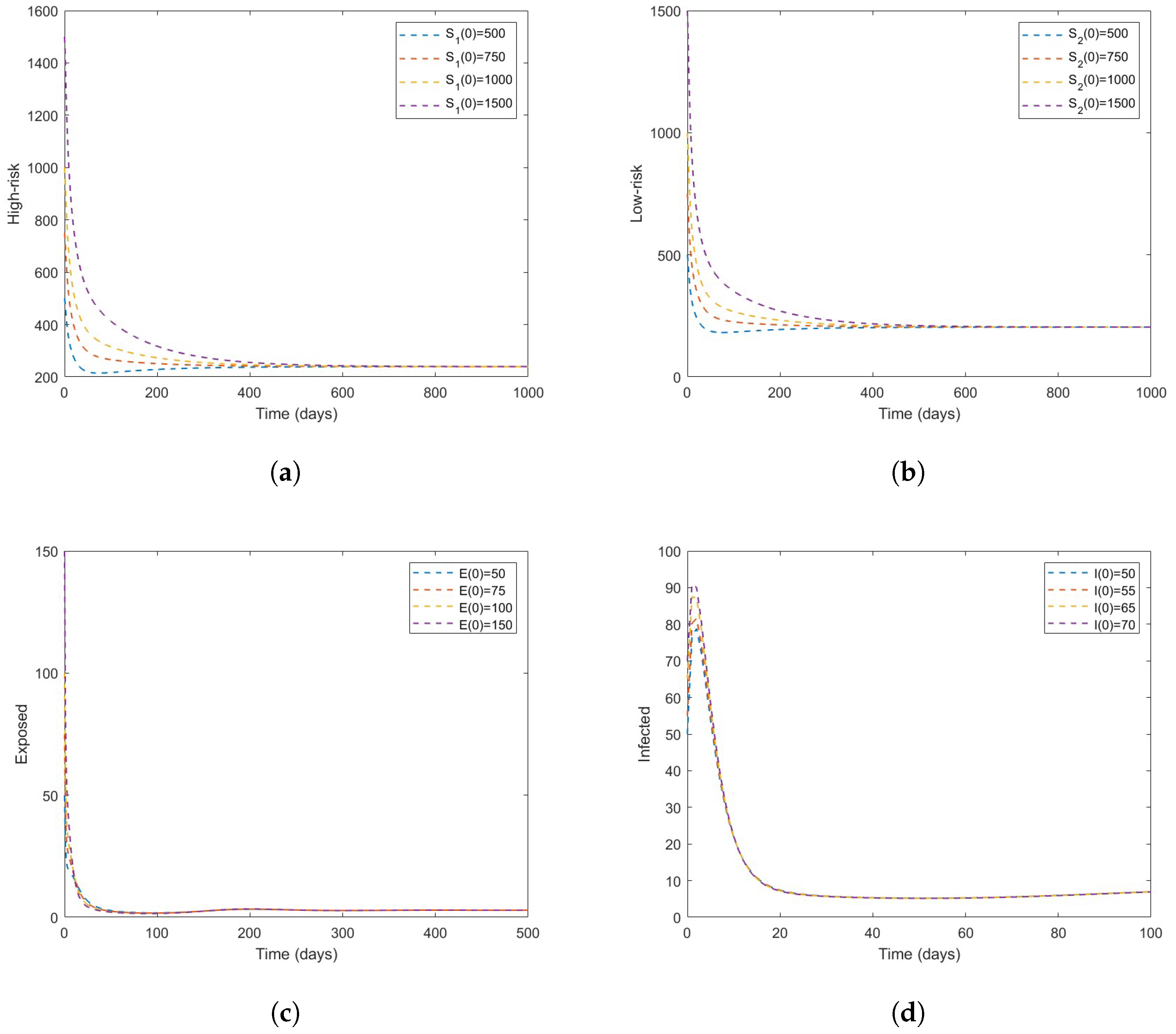
4. Numerical Simulations
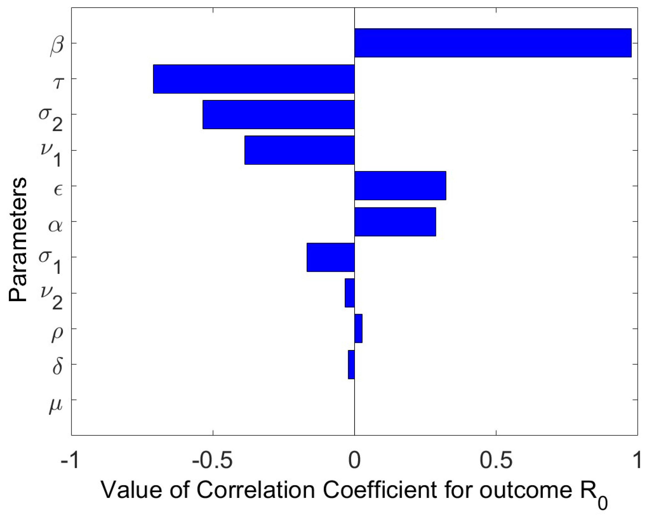
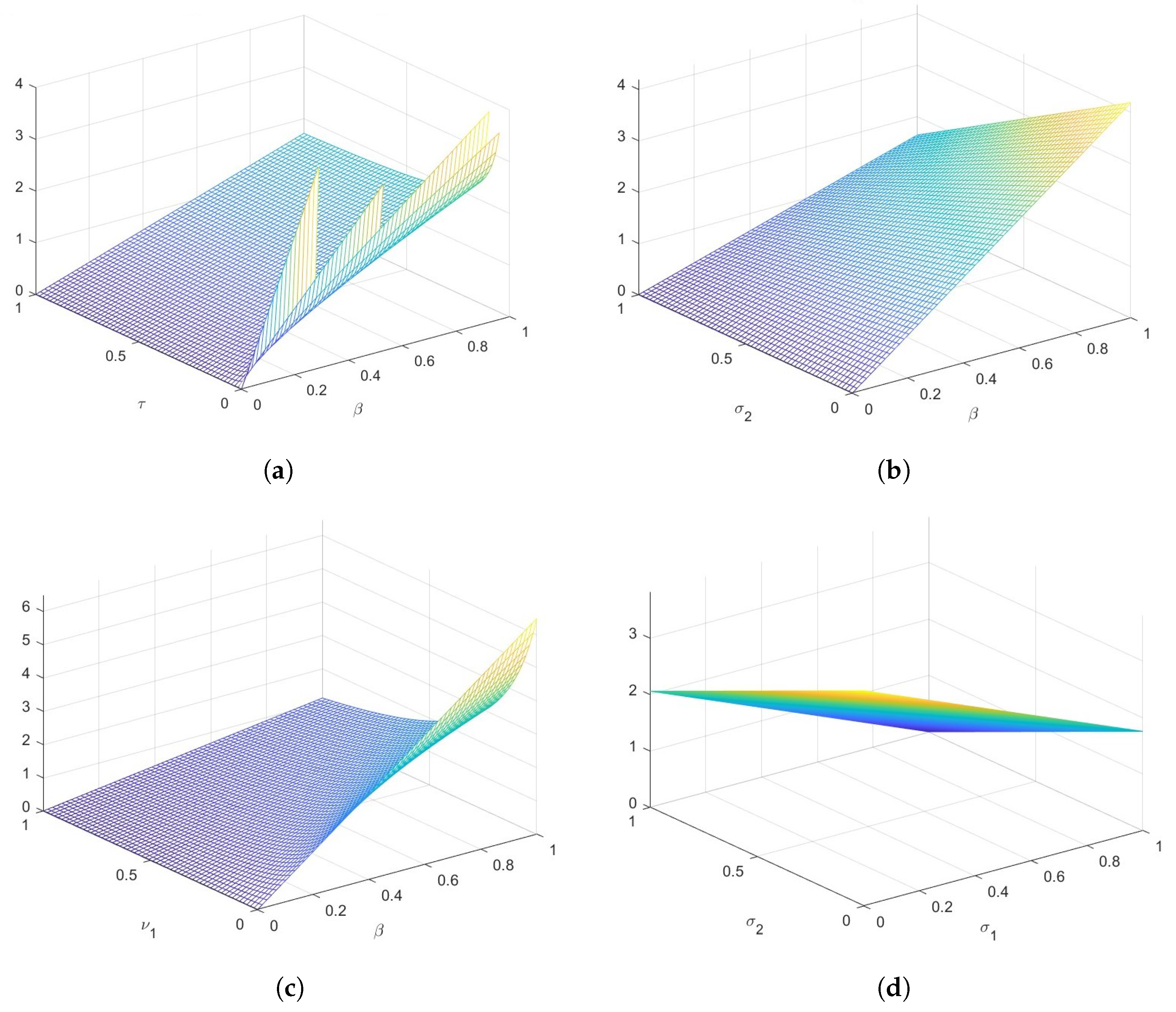
Sensitivity Analysis
5. Extended Model with Vaccination
- i.
- The number of high-risk individuals reduces.
- ii.
- Infections can be prevented with some degree of efficacy.
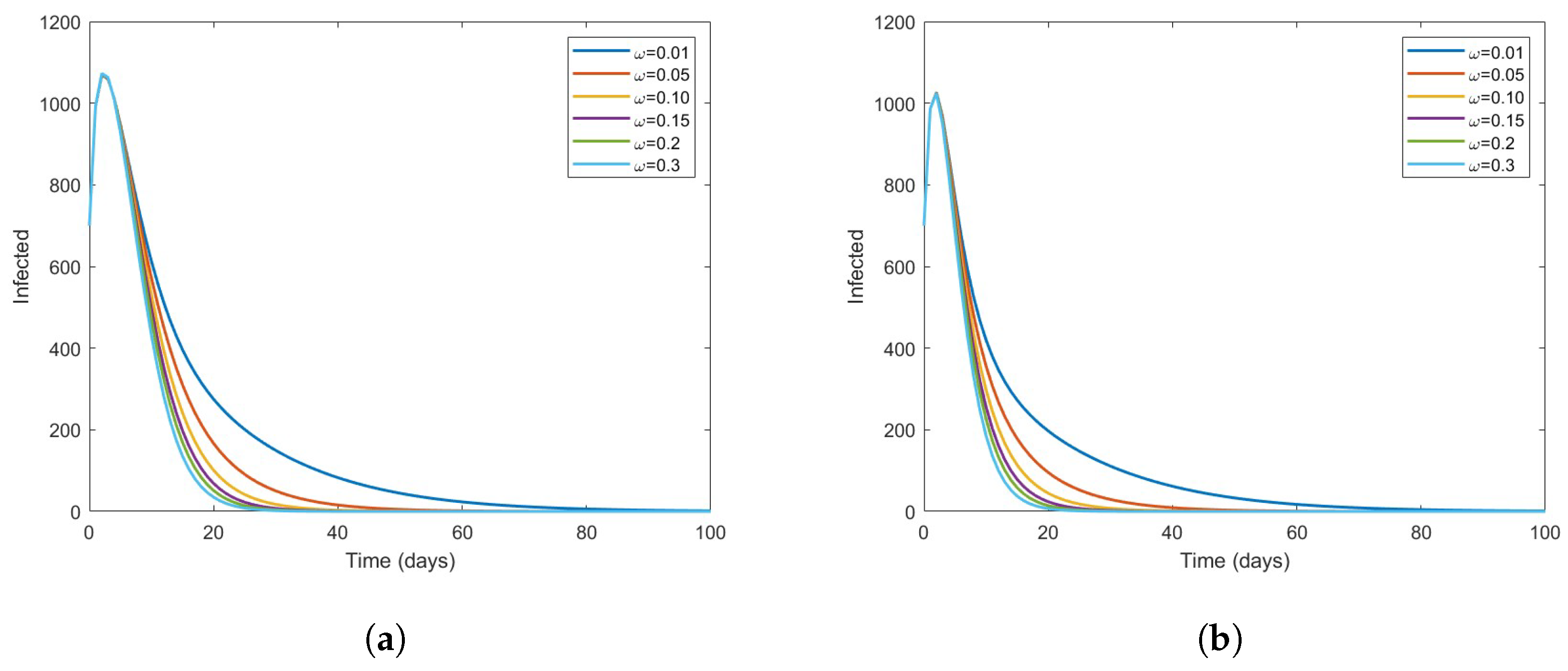
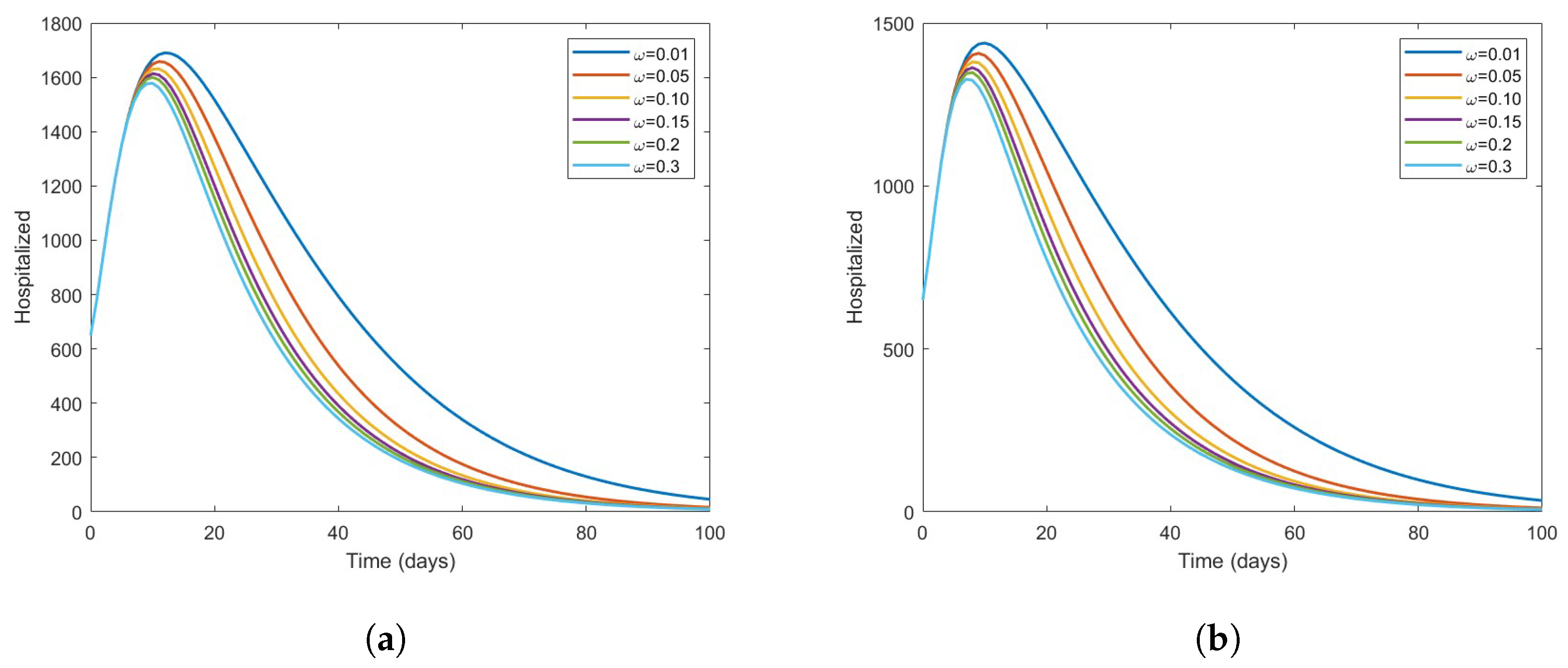
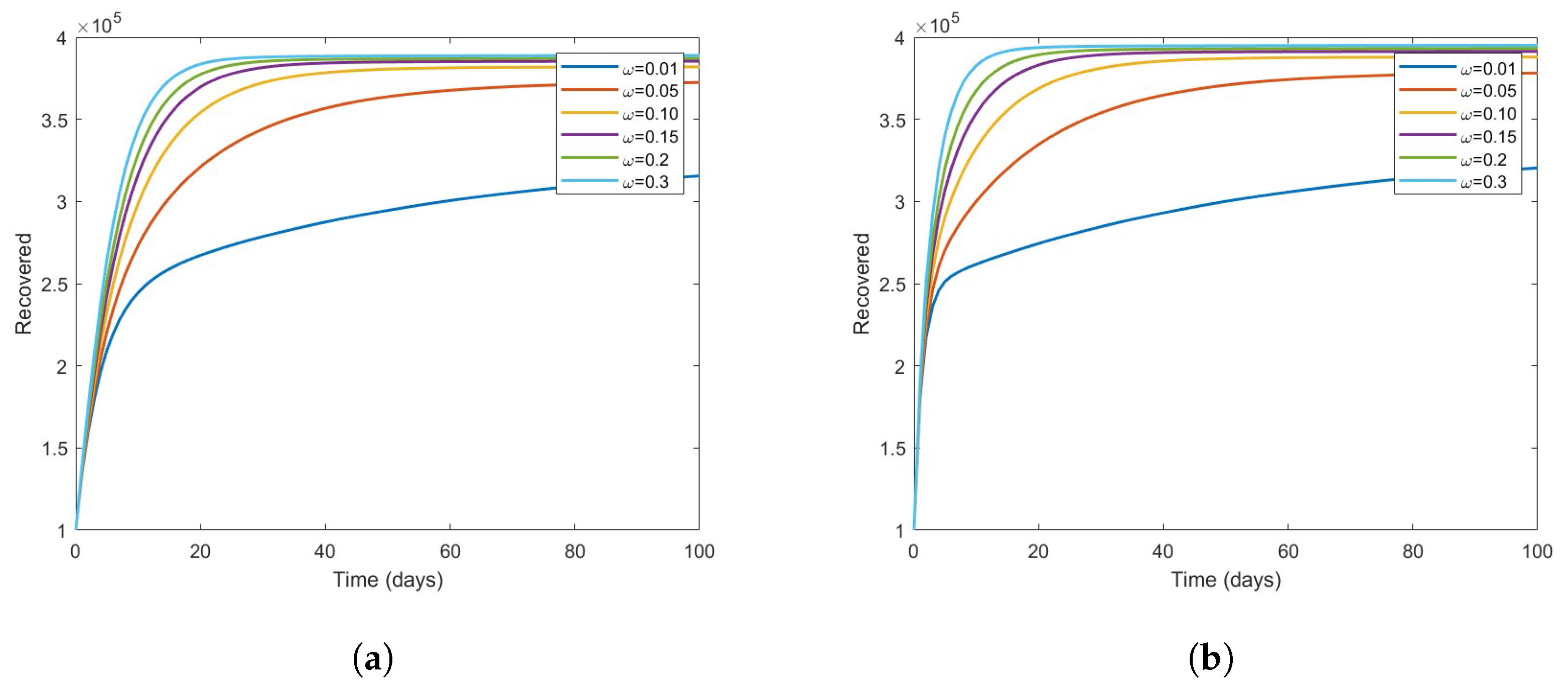
The Effect of Vaccine on the Disease Dynamics
6. Discussion and Conclusions
- (i)
- A GAS DFE occurs in the model without vaccination every time the associated basic reproduction number is less than 1 and there are multiple endemic equilibria, which is a GAS in a particular case.
- (ii)
- Based on numerical simulations it is indicated that if some high-risk individuals were vaccinated and moved to low-risk, the disease could be reduced to a minimum. However, this is dependent on the coverage of vaccinations.
- (iii)
- The Latin Hypercube Sampling to create 1000 samples and the resulting Partial Rank Correlation Coefficients (PRCCs) were used to perform a sensitivity study of the model parameter values. A tornado plot is used to visually display the results. The parameters , (hospitalized recovery rate), , (reduction in infectiousness of risk individuals), according to sensitivity analysis, greatly lessen an epidemic if increased. However, if the rates of person-to-person interaction and hospital inefficacy are reduced, transmission also decreases.
Future Work Directions
- Some new models with a different approach of incidence fraction can be proposed.
- Several dynamical features of COVID-19 were captured by our model, though other population compartments might be added and furthermore implement optimal control strategies when having access to more detailed and authentic COVID-19 data.
Supplementary Materials
Author Contributions
Funding
Data Availability Statement
Acknowledgments
Conflicts of Interest
Abbreviations
| COVID-19 | Coronavirus disease 2019 |
| NPIs | Non-pharmaceutical interventions against COVID-19 |
| DFE | Disease-free equilibrium |
| EE | Endemic equilibrium |
| LAS | Locally asymptotically stable |
| GAS | Globally asymptotically stable |
| SaSAT | Sampling and sensitivity analysis tool |
| PRCC | Partial rank correlation coefficient |
| LHS | Latin hypercube sampling |
| ASQ | Alternative state quarantine |
References
- Acter, T.; Uddin, N.; Das, J.; Akhter, A.; Choudhury, T.R.; Kim, S. Evolution of severe acute respiratory syndrome coronavirus 2 (SARS-CoV-2) as coronavirus disease 2019 (COVID-19) pandemic: A global health emergency. Sci. Total. Environ. 2020, 730, 138996. [Google Scholar] [CrossRef] [PubMed]
- Anderson, D.E.; Sivalingam, V.; Kang, A.E.Z.; Ananthanarayanan, A.; Arumugam, H.; Jenkins, T.M.; Hadjiat, Y.; Eggers, M. Povidone-iodine demonstrates rapid in vitro virucidal activity against SARS-CoV-2, the virus causing COVID-19 disease. Infect. Dis. Ther. 2020, 9, 669–675. [Google Scholar] [CrossRef] [PubMed]
- Elmancy, L.; Alkhatib, H.; Daou, A. SARS-CoV-2: An Analysis of the Vaccine Candidates Tested in Combatting and Eliminating the COVID-19 Virus. Vaccines 2022, 10, 2086. [Google Scholar] [CrossRef]
- Beach, B.; Clay, K.; Saavedra, M. The 1918 influenza pandemic and its lessons for COVID-19. J. Econ. Lit. 2022, 60, 41–84. [Google Scholar] [CrossRef]
- Ilatova, E.; Abraham, Y.S.; Celik, B.G. Exploring the Early Impacts of the COVID-19 Pandemic on the Construction Industry in New York State. Architecture 2022, 2, 457–475. [Google Scholar] [CrossRef]
- LaMattina, J.L. Pharma and Profits: Balancing Innovation, Medicine, and Drug Prices; John Wiley & Sons: Hoboken, NJ, USA, 2022. [Google Scholar]
- Vivian, D.T. Media Literacy and Fake News: Evaluating the Roles and Responsibilities of Radio Stations in Combating Fake News in the COVID-19 Era. Int. J. Inf. Manag. Sci. 2022, 6, 33–49. [Google Scholar]
- Hughes, D. What is in the so-called COVID-19 “Vaccines”? Part 1: Evidence of a Global Crime Against Humanity. Int. J. Vaccine Theory Pract. Res. 2022, 2, 455–586. [Google Scholar] [CrossRef]
- Kumari, M.; Lu, R.M.; Li, M.C.; Huang, J.L.; Hsu, F.F.; Ko, S.H.; Ke, F.-Y.; Su, S.-C.; Liang, K.-H.; Yuan, J.P.-Y. A critical overview of current progress for COVID-19: Development of vaccines, antiviral drugs, and therapeutic antibodies. J. Biomed. Sci. 2022, 29, 1–36. [Google Scholar] [CrossRef]
- Niknam, Z.; Jafari, A.; Golchin, A.; Danesh Pouya, F.; Nemati, M.; Rezaei-Tavirani, M.; Rasmi, Y. Potential therapeutic options for COVID-19: An update on current evidence. Eur. J. Med. Res. 2022, 27, 1–15. [Google Scholar] [CrossRef]
- Favilli, A.; Mattei Gentili, M.; Raspa, F.; Giardina, I.; Parazzini, F.; Vitagliano, A.; Borisova, A.V.; Gerli, S. Effectiveness and safety of available treatments for COVID-19 during pregnancy: A critical review. J. Matern.-Fetal Neonatal Med. 2022, 35, 2174–2187. [Google Scholar] [CrossRef]
- Graham, E.L.; Koralnik, I.J.; Liotta, E.M. Therapeutic approaches to the neurologic manifestations of COVID-19. Neurotherapeutics 2022 19, 1435–1466. [CrossRef]
- Md Khairi, L.N.H.; Fahrni, M.L.; Lazzarino, A.I. The race for global equitable access to COVID-19 vaccines. Vaccines 2022, 10, 1306. [Google Scholar] [CrossRef] [PubMed]
- Lukaszuk, K.; Podolak, A.; Malinowska, P.; Lukaszuk, J.; Jakiel, G. Cross-Reactivity between Half Doses of Pfizer and AstraZeneca Vaccines—A Preliminary Study. Vaccines 2022, 10, 521. [Google Scholar] [CrossRef] [PubMed]
- Liu, X.; Zhao, N.; Li, S.; Zheng, R. Opt-out policy and its improvements promote COVID-19 vaccinations. Soc. Sci. Med. 2022, 307, 115120. [Google Scholar] [CrossRef] [PubMed]
- Moore, S.; Hill, E.M.; Dyson, L.; Tildesley, M.J.; Keeling, M.J. Retrospectively modeling the effects of increased global vaccine sharing on the COVID-19 pandemic. Nat. Med. 2022, 28, 2416–2423. [Google Scholar] [CrossRef]
- Tyagi, S.; Martha, S.C.; Abbas, S.; Debbouche, A. Mathematical modeling and analysis for controlling the spread of infectious diseases. Chaos Solitons Fractals 2021, 144, 1107072. [Google Scholar] [CrossRef] [PubMed]
- Iboi, E.; Sharomi, O.O.; Ngonghala, C.; Gumel, A.B. Mathematical modeling and analysis of COVID-19 pandemic in Nigeria. MedRxiv 2020. [Google Scholar] [CrossRef]
- Riyapan, P.; Shuaib, S.E.; Intarasit, A. A mathematical model of COVID-19 pandemic: A case study of Bangkok, Thailand. Comput. Math. Methods Med. 2021, 2021, 6664483. [Google Scholar] [CrossRef]
- Tylicki, L.; Puchalska-Reglińska, E.; Tylicki, P.; Och, A.; Polewska, K.; Biedunkiewicz, B.; Parczewska, A.; Szabat, K.; Wolf, J.; Dębska-Ślizień, A. Predictors of mortality in hemodialyzed patients after SARS-CoV-2 infection. J. Clin. Med. 2022, 11, 285. [Google Scholar] [CrossRef]
- He, S.; Peng, Y.; Sun, K. SEIR modeling of the COVID-19 and its dynamics. Nonlinear Dyn. 2020, 101, 1667–1680. [Google Scholar] [CrossRef]
- Bajiya, V.P.; Bugalia, S.; Tripathi, J.P. Mathematical modeling of COVID-19: Impact of non-pharmaceutical interventions in India. Chaos Interdiscip. J. Nonlinear Sci. 2020, 30, 113143. [Google Scholar] [CrossRef] [PubMed]
- Chen, T.; Wu, D.; Chen, H.; Yan, W.; Yang, D.; Chen, G.; Ma, K.; Xu, D.; Yu, H.; Wang, H. Clinical characteristics of 113 deceased patients with coronavirus disease 2019: Retrospective study. BMJ 2020, 368, m1091. [Google Scholar] [CrossRef] [PubMed] [Green Version]
- Wang, C.; Horby, P.W.; Hayden, F.G.; Gao, G.F. A novel coronavirus outbreak of global health concern. Lancet 2020, 395, 470–473. [Google Scholar] [CrossRef] [PubMed] [Green Version]
- Mtisi, E.; Rwezaura, H.; Tchuenche, J.M. A mathematical analysis of malaria and tuberculosis co-dynamics. Discret. Contin. Dyn. Syst.-B 2009, 12, 827. [Google Scholar] [CrossRef]
- Prathumwan, D.; Trachoo, K.; Chaiya, I. Mathematical modeling for prediction dynamics of the coronavirus disease 2019 (COVID-19) pandemic, quarantine control measures. Symmetry 2020, 12, 1404. [Google Scholar] [CrossRef]
- Van den Driessche, P.; Watmough, J. Reproduction numbers and sub-threshold endemic equilibria for compartmental models of disease transmission. Math. Biosci. 2002, 180, 1–2. [Google Scholar] [CrossRef]
- La, S.; Joseph, P. The Stability of Dynamical Systems; Society for Industrial and Applied Mathematics: Philadelphia, PA, USA, 1976. [Google Scholar]
- Garba, S.M.; Gumel, A.B.; Bakar, M. Abu. Backward bifurcations in dengue transmission dynamics. Math. Biosci. 2008, 215, 11–25. [Google Scholar] [CrossRef]
- Roop, O.P.; Chinviriyasit, W.; Chinviriyasit, S. The effect of incidence function in backward bifurcation for malaria model with temporary immunity. Math. Biosci. 2015, 256, 47–64. [Google Scholar] [CrossRef]
- Yang, C.; Wang, X.; Gao, D.; Wang, J. Impact of awareness programs on cholera dynamics: Two modeling approaches. Bull. Math. Biol. 2017, 79, 2109–2131. [Google Scholar] [CrossRef] [Green Version]
- Salihu, S.M.; Shi, Z.; Chan, H.S.; Jin, Z.; He, D. A mathematical model to study the 2014–2015 large-scale dengue epidemics in Kaohsiung and Tainan cities in Taiwan, China. Math. Biosci. Eng. 2019, 6, 3841–3863. [Google Scholar]
- Asempapa, R.; Oduro, B.; Apenteng, O.O.; Magagula, V.M. A COVID-19 mathematical model of at-risk populations with non-pharmaceutical preventive measures: The case of Brazil and South Africa. Infect. Dis. Model. 2022, 7, 45–61. [Google Scholar] [CrossRef] [PubMed]
- Eikenberry, S.E.; Mancuso, M.; Iboi, E.; Phan, T.; Eikenberry, K.; Kuang, Y.; Kostelich, E.; Gumel, A.B. To mask or not to mask: Modeling the potential for face mask use by the general public to curtail the COVID-19 pandemic. Infect. Dis. Model. 2020, 5, 293–308. [Google Scholar] [CrossRef] [PubMed]
- Bala, S.I.; Gimba, B. Global sensitivity analysis to study the impacts of bed-nets, drug treatment, and their efficacies on a two-strain malaria model. Math. Comput. Appl. 2019, 24, 32. [Google Scholar] [CrossRef] [Green Version]
- Hoare, A.; Regan, D.G.; Wilson, D.P. Sampling and sensitivity analyses tools (SaSAT) for computational modelling. Theor. Biol. Med. Model. 2008, 5, 1–18. [Google Scholar] [CrossRef] [Green Version]
- Cianetti, S.; Pagano, S.; Nardone, M.; Lombardo, G. Model for taking care of patients with early childhood caries during the SARS-Cov-2 pandemic. Int. J. Environ. Res. Public Health 2020, 17, 3751. [Google Scholar] [CrossRef]
- Carli, E.; Pasini, M.; Pardossi, F.; Capotosti, I.; Narzisi, A.; Lardani, L. Oral Health Preventive Program in Patients with Autism Spectrum Disorder. Children 2022, 9, 535. [Google Scholar] [CrossRef]
- Baba, I.A.; Rihan, F.A. A fractional–order model with different strains of COVID-19. Phys. A Stat. Mech. Its Appl. 2022, 603, 127813. [Google Scholar] [CrossRef]
- Baba, I.A.; Sani, M.A.; Nasidi, B.A. Fractional dynamical model to assess the efficacy of facemask to the community transmission of COVID-19. Comput. Methods Biomech. Biomed. Eng. 2022, 25, 1588–1598. [Google Scholar] [CrossRef]


| Variables | Description |
|---|---|
| Number of high-risk susceptible population | |
| Number of low-risk susceptible population | |
| E | Number of exposed population |
| I | Number of infected population |
| H | Number of hospitalize population |
| R | Number of recovered population |
| N | Total human population |
| Parameter | Description |
|---|---|
| Recruitment rate | |
| Effective contact rate | |
| Fraction of newly recruited individuals moving to | |
| Rate of reduction in infectiousness in | |
| Rate of reduction in infectiousness in | |
| The natural death rate | |
| The rate of progression from exposed population to infected population | |
| The rate of hospital inefficacy | |
| The recovery rate of infected in | |
| The hospitalization rate of infected individuals | |
| The recovery rate of the hospitalized individuals | |
| The COVID-19 induced mortality rate |
Disclaimer/Publisher’s Note: The statements, opinions and data contained in all publications are solely those of the individual author(s) and contributor(s) and not of MDPI and/or the editor(s). MDPI and/or the editor(s) disclaim responsibility for any injury to people or property resulting from any ideas, methods, instructions or products referred to in the content. |
© 2022 by the authors. Licensee MDPI, Basel, Switzerland. This article is an open access article distributed under the terms and conditions of the Creative Commons Attribution (CC BY) license (https://creativecommons.org/licenses/by/4.0/).
Share and Cite
Ibrahim, A.; Humphries, U.W.; Khan, A.; Iliyasu Bala, S.; Baba, I.A.; Rihan, F.A. COVID-19 Model with High- and Low-Risk Susceptible Population Incorporating the Effect of Vaccines. Vaccines 2023, 11, 3. https://doi.org/10.3390/vaccines11010003
Ibrahim A, Humphries UW, Khan A, Iliyasu Bala S, Baba IA, Rihan FA. COVID-19 Model with High- and Low-Risk Susceptible Population Incorporating the Effect of Vaccines. Vaccines. 2023; 11(1):3. https://doi.org/10.3390/vaccines11010003
Chicago/Turabian StyleIbrahim, Alhassan, Usa Wannasingha Humphries, Amir Khan, Saminu Iliyasu Bala, Isa Abdullahi Baba, and Fathalla A. Rihan. 2023. "COVID-19 Model with High- and Low-Risk Susceptible Population Incorporating the Effect of Vaccines" Vaccines 11, no. 1: 3. https://doi.org/10.3390/vaccines11010003