Abstract
Separating non-ideal mixtures by pervaporation (hence PV) is a competitive alternative to most traditional methods, such as distillation, which are based on the vapour–liquid equilibrium (VLE). It must be said, in many cases, accurate VLE data are already well known in the literature. They make the method of PV modelling a lot more complicated, and most of the viable models are (semi)empirical and focus on component flux (Ji) estimation. The pervaporation model of Mizsey and Valentinyi, which is based on Rautenbach’s works, is further improved in this work and tested rigorously by statistical means. Until now, this type of exponential modelling was only used for alcohol–water mixtures, but in this work, it was extended to an ethyl acetate–water binary mixture as well. Furthermore, a flowchart of modelling is presented for the first time in the case of an exponential pervaporation model. The results of laboratory-scale experiments were used as the basis of the study and least squares approximation was used to compare them to the different model’s estimations. According to our results, Valentinyi’s model (Model I) and the alternative model (Model III) appear to be the best methods for PV modelling, and there is no significant difference between the models, mainly in organophilic cases. In the case of the permeation component, Model I, which better follows the exponential function, is recommended. It is important to emphasize that our research confirms that the exponential type model seems to be universally feasible for most organic–water binary mixtures. Another novelty of the work is that after PDMS and PVA-based membranes, the accuracy of the semiempirical model for the description of water flux on a PEBA-based membrane was also proved, in the organophilic case.
1. Introduction
Pervaporation (hence PV) is a type of membrane separation process, in which the components are separated by their different tendency to permeate through the membrane. On the feed side, the initial liquid is absorbed by the material of the polymer membrane and it is diffused through the length of the membrane, and then on the permeate side it is desorbed into the generated vacuum as a gas. In this type of process, the membrane is usually a composite membrane, which has an active and a porous supporting layer. The active layer is that which actually does the separation, by letting through the components at different degrees. The supporting layer does not take part in the separation—its only function is to provide mechanical stabilization. This is needed to counteract two forces: one is the hydrostatic pressure on the feed side, and the other one is the vacuum created on the permeate or product side [1,2].
Usually, during the separation of a binary solution, one of the components is water and the other one is an organic component. Depending on which is more likely to permeate through the membrane, there is hydrophilic (hence HPV) and organophilic pervaporation (hence OPV). There are several studies on organic–organic separation via PV, but these are not in the focus of this study [3,4,5,6].
The biggest advantage of PV, compared to the more traditional separation methods (such as distillation), is that it is not based on vapour–liquid equilibrium (hence VLE). Because of this, PV can be used to separate azeotropic solutions such as water–alcohol mixtures. So, even today, one of the most widely spread uses of PV is alcohol dehydration [7,8,9]. Further advantages are the capability of separating close-boiling point and heat-sensitive mixtures as well.
This VLE independency also poses a big problem when the aim is to model PV processes. Some of the most widely spread PV models are empirical or semiempirical [1,9], and so are heavily based on previous measurement, like in the case of the models discussed later in this work. One of best ways to characterise membrane processes is the component flux, which is the flowrate through a unit of membrane area [10]. So, it is not a surprise that most of the models focus on its estimation. Since this study focuses on the improvement of one of these models, the modelling of PV is mostly presented in the next chapter [11,12,13].
The aim of this work is to further develop a model that has been proven several times. By obtaining a better model, a more accurate calculation can support the PV process designing, via commercially used process simulation software (like ChemCAD and Aspen).
2. Materials and Methods
In this work, the examined aqueous mixtures can be seen in Table 1. PDMS (Sulzer PERVAP 4060), PVA (Sulzer PERVAP 1510) and, in the first case, PEBA pervaporation membranes were investigated. The standard deviation of the experimental data was 0.05. There were a minimum of three replicates in the experiments.

Table 1.
Examined mixtures.
2.1. Pervaporation Modelling
Modelling of traditional separation methods such as distillation is widely researched in literature [20,21]. The research field of distillation is heavily based on the vapour–liquid equilibrium (hence VLE). On the other hand, the mechanism of membrane separation cannot be explained by VLE. One of the most basic models that can be used for membrane separation is the diffusive or pore flow model.
In this case, the driving force of the separation is the chemical potential gradient between the two sides of the membrane. Because of the constant pressure in the membrane, the chemical potential gradient can be replaced with the concentration gradient. In this way, it is easier to define one of the most important parameters of pervaporation, the membrane flux, which can be described by Fick’s first law:
Since this is a general model for most transport processes, in this context ci is the concentration outside of the membrane.
The biggest drawback of this simplistic equation is the concentration dependency of the diffusion coefficient for non-ideal mixtures. For years, the scientific community have been working on the improvement of PV models for reliable flowsheet modelling uses.
Several pervaporation models have been brought forth as viable alternatives, such as the total solvent volume fraction model, pore-flow model and solution-diffusion model [12,22,23,24]. The solution diffusion one is quite probable theory; however, there are other theories to explain the complex phenomena of this membrane process. These theories are all only hypotheses and the authors know no experiment to prove them. One of the most widely accepted explanations is the solution-diffusion model, which is applicable for two-layered composite membranes. The model can be described by the following steps [12,25]:
- absorption of components in the membrane;
- selective diffusion of components through the length of the membrane;
- desorption and consequential evaporation to vapour phase on the permeate side.
This is the model on which Rautenbach’s (1990) [25] work is based. In his work, the driving force of the chemical potential gradient is replaced by the fugacity gradient, and the diffusion coefficient is replaced by the transport coefficient. The latter change is significant because of the lesser concentration dependency of the transport coefficient [26].
Based on Fick’s equation (Equation (1)), the component flux can be described as follows:
where is the geometric mean of the activity coefficient at the two sides of the composite membrane:
Introducing the transport coefficient:
Using the transport coefficient Equation (2) can be modified into:
Because the pressure at the permeate side is very low, the gas phase can be considered an ideal gas, and thus the fugacity difference can be replaced by partial pressure difference. Based on this, the partial flux can be defined as:
If Equation (5) is only determined for the active layer of the composite membrane and pressure is introduced instead of fugacity, combined with Equation (6), flux can by expressed as:
Transport coefficient can be calculated by the following Arrhenius type equation:
where T* is the reference temperature, in this case equal to 293 K or 20 °C.
In the works of Mizsey and Valentinyi [26,27], Rautenbach’s equation (Equation (7)) was modified and developed into the following:
This equation is called Model I in the work of Valentinyi et al. (2013) [27] (also, the original Rautenbach model is Equation (7)). It is generally accepted that the diffusion coefficient has an intense dependence on the feed concentration. Many authors have proposed an exponential relationship between the feed concentration and diffusion coefficient, which justifies the inserting of an exponential term into the pervaporation model [10,27]. This developed model is based on empirical laboratorial data [28,29], and it is specifically recommended for polymer and composite membranes.
Furthermore, in Mizsey’s work (2005) [26], it was established that the first part of Equation (7) as well as Equation (9) can be ignored. The reasoning behind this is that the porous supporting layer’s permeability coefficient (Q0) is infinitely big compared to the transport coefficient, correlating with the concept that this layer’s resistance is negligible. Thus, the Model I can be simplified as:
In this work, this equation was further improved as the following two models and researched in a similar fashion:
These models are called Model II and Model III, respectively.
2.2. Model Improvement
As mentioned, the model research is based on empirical laboratorian data [10,14,15,16,17,18,19]. For the calculations, the following base parameters were needed:
- mole fraction of the feed (xi1) [mole/mole];
- mole fraction of the permeate (xi3) [mole/mole];
- coefficients of the Wilson equation (Aij, Aji) [cal/moleK];
- input temperature (T) [°C. K];
- constants of the Antoine equation for both components (A, B, C, D and E) [-];
- pressure on the permeate side (p3) [bar. kPa];
- partial fluxes of both components (Ji) [kg/m2h].
The Antoine constants and Wilson parameters were obtained from the ChemCAD software’s database. Lower index numbers, as in the case of xi1 and p3, represent the location in the membrane module: 1 is the feed side, 2 is the intermembrane plane and 3 is the permeate side.
Based on these input parameters the following calculations can be executed. The activity coefficients can be calculated by the Wilson equation for both sides of the membrane and for both components. For example, for the component i, the feed side activity coefficient is:
where the Λij and Λji coefficients were obtained by the following formulas:
where the Vi and Vj are the molar volume of pure liquid. and it can be calculated as follows:
where A, B, C and D are the constants of the Antoine equation for the i and j components, respectively.
The pure component’s partial pressures can be calculated by the Antoine equation:
where A, B, C, D and E are the material depending constants of the Antoine equation.
Partial pressure in the feed and permeate side can be calculated by the Raoult’s law (Equation (17)) and Dalton’s law (Equation (18)), respectively:
To compare Model I, II and III, parameter fitting was used, for this purpose STATISTICA software was used. The estimated parameters were the reference transport coefficient (). component’s activation energy (Ei) and the added B parameter of the new models. The estimated function derives from the combination of the respective model and Equation (8):
As this is a nonlinear estimation process, a custom loss function needs to be defined, so least squares approximation was used. The objective function (hence OF) which needed to be minimized is the following:
For better transparency, the calculation method that was used in this work is represented on a flowchart (Figure 1).
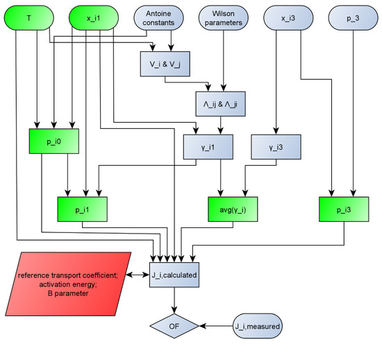
Figure 1.
Flowchart of calculation of pervaporation modelling. (Interpretation: p_i0 means pi0, others can be interpreted the same way and avg(y_i) means . Green parameters are the inputs of STATISTICA software. Red parameters are the parameters estimated by STATISTICA software.)
3. Results
As mentioned in the previous section, PV is mostly characterized by component flux, so during the model research it was estimated. To minimize the error, least squares approximation was used, and objective functions were obtained (Equation (22)), which can be seen in Table 2.
Table 2.
Objective functions in the case of different models.
Based on these OFs, it can be determined which model describes real measurement most accurately. The model that has the smallest OF in any case can be considered to be more accurate.
As stated before, the examined models use three estimated parameters: the reference transport coefficient (), the component’s activation energy (Ei), and the added B parameter. Estimation of these parameters can be seen in Table 3 for each component.
Table 3.
Estimated function parameters in case of the best model for each component.
4. Discussion
As can be seen in Table 2., Model II gave the biggest OFs in all cases, so it did not provide us with any promise of progression. On the other hand, Model III in some cases provided even better results than Valentinyi’s Model I.
In most cases, Model III proved to be better with regard to water flux modelling than Model I. These cases can be seen in Table 2 and as a representation in Figure 2a. Some cases, such as the water flux for OPV separation of isobutanol and water, are not too meaningful, but are still noticeable via OFs. The only exception is the HPV separation of isobutanol and water, where Model I beats the otherwise dominant Model III.
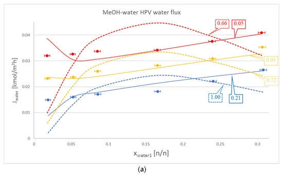
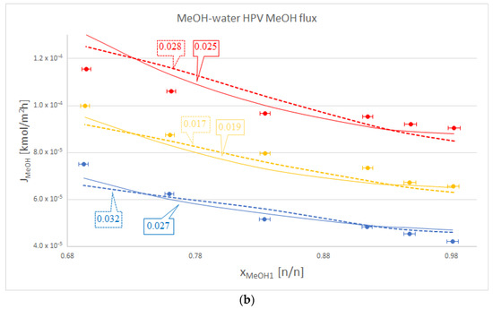
Figure 2.
Comparison of Model I (- - -), Model III (–––) and experimental data (●), where the colour code means the following: blue: 50 °C, yellow: 60 °C and red: 70 °C. Objective functions (OFs) are represented in the text bubbles per model per temperature. (a) MeOH-water hydrophilic (HPV) water flux; (b) MeOH-water HPV MeOH flux.
It is also worth mentioning that in the case of the organic component, Model III did not lag behind by much compared to Model I. This can be seen in Table 2., in the iBuOH-water and the first EtAc-water OPV results. In some cases, like both OPV and HPV separation of MeOH-water, Model III it is even better.
OFs were also analysed by temperature, so it can be determined whether the models work better at higher or lower temperature zones. OFs sorted by temperatures and mixture can be seen in Table 4. Overall, it can be said that both models behave similarly depending temperature changes and, in most cases, aqueous and organic component modelling is also indifferent. There is not a universal trend for temperature dependency, but most often higher temperatures yield lower OF. This observation needs further and bigger scale examination.
Table 4.
Objective functions temperature dependency.
Just like in other works, our models aim to estimate the partial flux for different components, heavily based on Fick’s law (Equation (1)), and make a lot of the same assumptions and simplifications. However, the goal of most models is to find a universal linear function; meanwhile, our approach keeps the exponential expression and changes its parameter to achieve a better fit to empirical data. Another difference is that other models use the plasticisation coefficient and partial activity to estimate the locational changes of the diffusion coefficient [30], or further boundary conditions are given to achieve an Arrhenius-type equation for partial flux [31]. Some cases just use the concentration to get a linear model for liquid composition estimation in the membrane [32], while our model uses fugacity and partial pressure to achieve an exponential empirical equation. Even more complicated models use the thermodynamic functions of solubility as well as diffusion [33], while ours only uses the latter.
5. Conclusions
In this work, two new alternative models were proposed for component flux estimation in pervaporation processes, Model II and III. Of those two, Model II seems to be less accurate than Valentinyi’s established Model I, so no further research is worthwhile. Meanwhile, Model III seems to be better in some regards, such as in water flux estimation for OPV processes. In most cases there is little difference between Model I and III in organic flux estimation for OPV processes. Overall, it can be said that further examination is needed for the investigation of this model, but it is more than promising.
In this study, it was also determined that both Model I and III behave similarly regarding temperature changes, and at higher temperatures the models yield more realistic approximations. However, for this type of study, bigger input data are needed, so it should be researched further.
To summarise, the recommended models for the examined mixtures are listed in Table 5. The model in parentheses is also correct but less accurate. As can be mentioned, in most cases the new Model III is better in the estimation of water flux, while Model I is better for organic component flux estimation.
Table 5.
Recommended model for examined mixtures.
Model I more closely follows the nature of the exponential function, which is more compatible with the permeable target component. In conclusion, the two models describe the flux of pervaporation with sufficient accuracy. Model I is universal, while Model III can be used for the non-target component because there is no significant difference between the two models.
It must be mentioned that the exponential type model was extended to an ethyl acetate–water binary mixture, as only alcohol–water binary mixtures were examined until now. The data show that both models can work just as well for ethyl acetate as they do in the case of alcohols. So, the exponential type model most likely describes the majority of organic–water binary mixtures.
Author Contributions
Conceptualization, A.J.T.; methodology, B.S.; writing—review and editing, B.S. All authors have read and agreed to the published version of the manuscript.
Funding
This publication was supported by the János Bolyai Research Scholarship of the Hungarian Academy of Sciences, NTP-NFTÖ-20-B-0095 National Talent Program of the Cabinet Office of the Prime Minister, OTKA 128543 and 131586. This research was supported by the European Union and the Hungarian State, co-financed by the European Regional Development Fund in the framework of the GINOP-2.3.4-15-2016-00004 project, aimed to promote the cooperation between the higher education and the industry. The research reported in this paper and carried out at the Budapest University of Technology and Economics has been supported by the National Research Development and Innovation Fund (TKP2020 National Challenges Subprogram, Grant No. BME-NC) based on the charter of bolster issued by the National Research Development and Innovation Office under the auspices of the Ministry for Innovation and Technology.
Conflicts of Interest
The authors declare no conflict of interest.
Nomenclature
| A | membrane area [m2] |
| B | constant in Model I, II and III |
| c | total molar concentration [mol/mol] |
| ci | concentration of component i [mol/m3] |
| Di | diffusion coefficient [m2/h] |
| Di0 | diffusion coefficient of component i [ kmol/m2 h] |
| transport coefficient of component i [kmol/m2 h] | |
| modified transport coefficient of component i in Model I, II and III [kmol/m2 h] | |
| relative transport coefficient of component i [kmol/m2 h] | |
| Ei | activation energy of component i [kJ/mol] |
| fi0 | fugacity of pure i component [mbar, kPa] |
| fi1 | fugacity of component i in the feed side [mbar, kPa] |
| fi3 | fugacity of component i in the permeate side [mbar, kPa] |
| J | total flux [kg/m2h] |
| Ji | partial flux [kg/m2h] |
| L | distance of diffusion [m] |
| ni | weight of component i [mol] |
| pi0 | vapour pressure of pure i component [bar, kPa] |
| pi1 | partial pressure of component i in the feed side [bar, kPa] |
| pi2 | partial pressure of component i between the two layers of the membrane [bar, kPa] |
| pi3 | partial pressure of component i in the permeate side [bar, kPa] |
| p3 | pressure on the permeate side [bar, kPa] |
| Q0 | permeability of the porous supporting layer of the membrane [kmol/m2 h bar] |
| R | gas constant [kJ/kmol K] |
| t | time [s, h] |
| T | temperature [K, °C] |
| T* | reference temperature: 273 K = 20 °C |
| wF | feed concentration of component i [wt%] |
| xi1 | mol fraction of component i in the feed [mol/mol] |
| yi | mol fraction of component i in the permeate [mol/mol] |
| Greek letters: | |
| βij | selectivity for component i and j |
| δ | thickness of the membrane [m] |
| γi1 | activity coefficient of component i in the feed |
| γi3 | activity coefficient of component i in the permeate |
| average activity coefficient of component i |
References
- Figoli, A.; Santoro, S.; Galiano, F.; Basile, A. Pervaporation membranes: Preparation characterization and application. In Pervaporation, Vapour Permeation and Membrane Distillation; Basile, A., Figoli, A., Khayet, M., Eds.; Woodhead Publishing: Cambridge, UK, 2015; Volume 1, pp. 19–63. [Google Scholar]
- Heintz, A.; Stephan, W. A generalized solution—Diffusion model of the pervaporation process through composite membranes Part I. Prediction of mixture solubilities in the dense active layer using the UNIQUAC model. J. Membr. Sci. 1994, 89, 143–151. [Google Scholar] [CrossRef]
- Penkova, A.V.; Pientka, Z.; Polotskaya, G.A. MWCNT/poly(phenylene isophtalamide) Nanocomposite Membranes for Pervaporation of Organic Mixtures. Fuller. Nanotub. Carbon Nanostruct. 2010, 19, 137–140. [Google Scholar] [CrossRef]
- Smitha, B.; Suhanya, D.; Sridhar, S.; Ramakrishna, M. Separation of organic-organic mixtures by pervaporation—a review. J. Membr. Sci. 2004, 241, 1–21. [Google Scholar] [CrossRef]
- Tang, J.; Sirkar, K.K.; Majumdar, S. Permeation and sorption of organic solvents and separation of their mixtures through an amorphous perfluoropolymer membrane in pervaporation. J. Membr. Sci. 2013, 447, 345–354. [Google Scholar] [CrossRef]
- Zhang, Q.G.; Han, G.L.; Hu, W.W.; Zhu, A.M.; Liu, Q.L. Pervaporation of Methanol–Ethylene Glycol Mixture over Organic–Inorganic Hybrid Membranes. Ind. Eng. Chem. Res. 2013, 52, 7541–7549. [Google Scholar] [CrossRef]
- Ling, W.S.; Thian, T.C.; Bhatia, S. Process optimization studies for the dehydration of alcohol–water system by inorganic membrane based pervaporation separation using design of experiments (DOE). Sep. Purif. Technol. 2010, 71, 192–199. [Google Scholar] [CrossRef]
- Liu, P.; Chen, M.; Ma, Y.; Hu, C.; Zhang, Q.; Zhu, A.; Liu, Q. A hydrophobic pervaporation membrane with hierarchical microporosity for high-efficient dehydration of alcohols. Chem. Eng. Sci. 2019, 206, 489–498. [Google Scholar] [CrossRef]
- Schiffmann, P.; Repke, J.-U. Design of pervaporation modules based on computational process modelling. Comput. Aided Chem. Eng. 2011, 29, 397–401. [Google Scholar] [CrossRef]
- Toth, A.J.; Andre, A.; Haaz, E.; Mizsey, P. New horizon for the membrane separation: Combination of organophilic and hydrophilic pervaporations. Sep. Purif. Technol. 2015, 156, 432–443. [Google Scholar] [CrossRef]
- Lipnizki, F.; Trägårdh, G. Modeling of pervaporation: Models to analyze and predict the mass transport in pervaporation. Sep. Purif. Rev. 2007, 30, 49–125. [Google Scholar] [CrossRef]
- Schaetzel, P.; Vauclair, C.; Nguyen, Q.T.; Bouzerar, R. A simplified solution–diffusion theory in pervaporation: The total solvent volume fraction model. J. Membr. Sci. 2004, 244, 117–127. [Google Scholar] [CrossRef]
- Sukitpaneenit, P.; Chung, T.-S.; Jiang, L.Y. Modified pore-flow model for pervaporation mass transport in PVDF hollow fiber membranes for ethanol–water separation. J. Membr. Sci. 2010, 362, 393–406. [Google Scholar] [CrossRef]
- Haaz, E.; Valentinyi, N.; Tarjani, A.J.; Fozer, D.; Andre, A.; Asmaa, S.; Rahimli, F.; Nagy, T.; Mizsey, P.; Deak, C.; et al. Platform molecule removal from aqueous mixture with organophilic pervaporation: Experiments and modelling. Period. Polytech. Chem. Eng. 2019, 63, 138–146. [Google Scholar] [CrossRef]
- Virag, B. Investigation of Ethanol-Water Mixture with Organophilic Pervaporation. Master’s Thesis, Budapest University of Technology and Economics, Budapest, Hungary, 2007. [Google Scholar]
- Toth, A.J.; Andre, A.; Haaz, E.; Nagy, T.; Valentinyi, N.; Fozer, D.; Mizsey, P. Application of pervaporation and distillation for utilization process wastewaters. In Proceedings of the Hungarian Water- and Wastewater Association Dr. Dulovics Dezső Junior Symposium, Budapest, Hungary, 22 March 2018. [Google Scholar]
- Poraczki, A. Investigation of Separation of Ethyl Acetate–Water Mixture with Pervaporation. Master’s Thesis, Budapest University of Technology and Economics, Budapest, Hungary, 2016. [Google Scholar]
- Vatani, M.; Raisi, A.; Pazuki, G. Mixed matrix membrane of ZSM-5/poly (ether-block-amide)/polyethersulfone for pervaporation separation of ethyl acetate from aqueous solution. Microporous Mesoporous Mater. 2018, 263, 257–267. [Google Scholar] [CrossRef]
- Haaz, E.; Toth, A.J. Methanol dehydration with pervaporation: Experiments and modelling. Sep. Purif. Technol. 2018, 205, 121–129. [Google Scholar] [CrossRef]
- Wesselingh, J.A. Non-Equilibrium Modelling of Distillation. Chem. Eng. Res. Des. 1997, 75, 529–538. [Google Scholar] [CrossRef]
- Tränkle, F.; Gerstlauer, A.; Zeitz, M.; Gilles, E.D. Application of the modeling and simulation environment ProMoT/Diva to the modeling of distillation processes. Comput. Chem. Eng. 1997, 21, S841–S846. [Google Scholar] [CrossRef]
- Heintz, A.; Stephan, W. A generalized solution–diffusion model of the pervaporation process through composite membranes Part II. Concentration polarization, coupled diffusion and the influence of the porous support layer. J. Membr. Sci. 1994, 89, 153–169. [Google Scholar] [CrossRef]
- Marriott, J.; Sørensen, E. A general approach to modelling membrane modules. Chem. Eng. Sci. 2003, 58, 4975–4990. [Google Scholar] [CrossRef]
- Wijmans, J.G.; Baker, R.W. The solution-diffusion model: A review. J. Membr. Sci. 1995, 107, 1–21. [Google Scholar] [CrossRef]
- Rautenbach, R.; Herion, C. Meyer-Blumentoth, U. Pervaporation membrane separation processes. Membr. Sci. Technol. Ser. 1990, 1, 181–191. [Google Scholar]
- Mizsey, P.; Koczka, K.; Deák, A.; Fonyó, Z. Simulation of pervaporation using the “solution–diffusion” model. Hung. Chem. J. 2005, 7, 239–242. [Google Scholar]
- Valentínyi, N.; Cséfalvay, E.; Mizsey, P. Modelling of pervaporation: Parameter estimation and model development. Chem. Eng. Res. Des. 2013, 91, 174–183. [Google Scholar] [CrossRef]
- Himics, M. Examination of Pervaporation Modeling Determination of Model Parameters in the Case of Butanol–Water Mixture. Bachelor’s Thesis, Budapest University of Technology and Economics, Budapest, Hungary, 2009. [Google Scholar]
- Koczka, K. Environmental Conscious Design and Industrial Application of Separation Processes. Ph.D. Thesis, Budapest University of Technology and Economics, Budapest, Hungary, 2009. [Google Scholar]
- Ortiz, I.; Gorri, D.; Casado, C.; Urtiaga, A. Modelling of the pervaporative flux through hydrophilic membranes. J. Chem. Technol. Biotechnol. 2005, 80, 397–405. [Google Scholar] [CrossRef]
- Gonzalez, B.; Ortiz, I. Mathematical Modeling of the Pervaporative Separation of Methanol–Methylterbutyl Ether Mixtures. Ind. Eng. Chem. Res. 2001, 40, 1720–1731. [Google Scholar] [CrossRef]
- Matsui, S.; Paul, D.R. A simple model for pervaporative transport of binary mixtures through rubbery polymeric membranes. J. Membr. Sci. 2004, 235, 25–30. [Google Scholar] [CrossRef]
- Ebneyamini, A.; Azimi, H.; Tezel, F.H.; Thibault, J. Modelling of mixed matrix membranes: Validation of the resistance-based model. J. Membr. Sci. 2017, 543, 361–369. [Google Scholar] [CrossRef]


Publisher’s Note: MDPI stays neutral with regard to jurisdictional claims in published maps and institutional affiliations. |
© 2020 by the authors. Licensee MDPI, Basel, Switzerland. This article is an open access article distributed under the terms and conditions of the Creative Commons Attribution (CC BY) license (http://creativecommons.org/licenses/by/4.0/).