Agricultural Risk Management Using Fuzzy TOPSIS Analytical Hierarchy Process (AHP) and Failure Mode and Effects Analysis (FMEA)

Abstract

Failure mode and effects analysis (FMEA) is a popular technique in reliability analyses. In a typical FMEA, there are three risk factors for each failure modes: Severity (S), occurrence (O), and detectability (D). These will be included in calculating a risk priority number (RPN) multiplying the three aforementioned factors. The literature review reveals some noticeable efforts to overcome the shortcomings of the traditional FMEA. The objective of this paper is to extend the application of FMEA to risk management for agricultural projects. For this aim, the factor of severity in traditional FMEA is broken down into three sub-factors that include severity on cost, the severity on time, and severity on the quality of the project. Moreover, in this study, a fuzzy technique for order preference by similarity to ideal solution (TOPSIS) integrated with a fuzzy analytical hierarchy process (AHP) was used to address the limitations of the traditional FMEA. A sensitivity analysis was done by weighing the risk assessment factors. The results confirm the capability of this Hybrid-FMEA in addressing several drawbacks of the traditional FMEA application. The risk assessment factors changed the risk priority between the different projects by affecting the weights. The risk of water and energy supplies and climate fluctuations and pests were the most critical risk in agricultural projects. Risk control measures should be applied according to the severity of each risk. Some of this research’s contributions can be abstracted as identifying and classifying the risks of investment in agricultural projects and implementing the extended FMEA and multicriteria decision-making methods for analyzing the risks in the agriculture domain for the first time. As a management tool, the proposed model can be used in similar fields for risk management of various investment projects.

1. Introduction

Agriculture industry is significantly challenged with numerous risks and uncertainties in project management. Advancement of the novel methods for risk assessment and project management is of significant importance [1]. Among the economic sectors, capital investment in the agriculture sector has a special position since it provokes a growth in the production and employment [2]. It also promotes production and economic growth [2]. The agriculture section confronts a capital escape due to an incapability to compete with the industry and the service sector and have a higher risk activity than other fields [3]. Generally, the agricultural sector includes a more risk level than the other sectors [4]. In fact, weather conditions and other natural phenomena make agriculture risky [5]. Moreover, there are other affecting factors like changes in the agricultural products’ prices, fertilizers and the other input as well as financial and political uncertainties in this field [6,7,8,9,10,11]. Agriculture risk management has been in the focal attention of many organizations active in this domain, especially in developing countries [12,13]. A lot of policymakers are still looking for a way to build an effective and efficient risk management support system in agriculture [14,15]. A lot of researchers and experts have paid attention to the risk management subject in the agricultural supply chain. Supply chains in the food industry are more complicated than other supply chains because of the perishability of food compared to other commodities [16,17].

Multiple studies say that organizations need a formal structure for identifying and evaluating the risks in supply chain and implementing a plan for mitigating the risks to minimize food wastage [18,19]. Investigating food supply chains risks can enhance the performance of these supply chains [20]. One of the most applied tools in evaluating and managing risk, is the failure mode and effects analysis (FMEA) method. FMEA is a technique that is applied in a many various areas. Moreover, FMEA has been widely used in the food industry to assess risks in the food production process [21]. This method has been used in determining the risks in the agricultural supply chain for identifying the risk of damage or lost quality and product contamination throughout the entire supply chain [22].

While there are many articles on the application of FMEA in the food supply chain risk domain and the risk of food products production, this method has not been used in evaluating agriculture plans yet and we cannot find valid articles in this field. The majority of the studies related to agricultural risk management have focused on the agricultural engineering and control of the environmental factors and the Project risk management tools are less used in this field. While Girdziute [10] introduced methods in their article such as Fuzzy matrix, Event tree analysis (ETA), Fault tree analysis (FTA), Delphi technique, and Monte-Carlo simulation for evaluating agricultural risks, but studies focusing on the comprehensive evaluation and comparison of the different agricultural risks are rare. Based on the investor needs, that is agricultural risk management from the preparation to the exploitation stage, common characteristics in the agricultural plans and the other projects as well as the similarity of the risks existing in the agricultural sector and project management, this article aims at using the existing tools of project risk management in the agricultural sector. Therefore, each agricultural plan can be considered as a project containing construct and exploitation time, the cost and quality of exploitation. This research addresses the following research questions:

• What are the main risks of agriculture plans?
• What are the proper measures for evaluating the risk of under-study agriculture plans risk?
• How can one evaluate and rank the identified risks based on the sensitivity of time, cost, and quality dimensions in each agriculture plan?
• How can one rank the identified risks considering all the agriculture plans?

Proposing a framework can equip the investors for evaluating risk and comparing their investment plans. For this aim, the FMEA method is chosen for agricultural projects risk management. FMEA is a tool mostly used for safety and reliability analysis of products and processes; however, several studies suggest using FMEA in the context of project risk management [23]. FMEA method can be used in project risk management due to its ease of use, familiar format, and comprehensive structure [24,25]. This technique was recommended by international standards such as MIL-STD-1629A [26]. In the traditional FMEA, the ranking of critical failure modes is performed via risk priority numbers (RPN) that is a product of evaluating some factors such as occurrence probability (O), severity (S), and detection (D) of each failure mode: RPN = S*O*D. This index describes the priority of the risk levels corresponding each failure mode [27]. Despite the wide application of FMEA in different domains, researchers criticize it because of the probability of error, contradiction, and ambiguity in judging the entering variables, the probability of producing the same RPN while the different set of entering variables, not taking into account the relative importance of the entering parameters, not considering indirect relations between parameters and so on [28,29,30,31]. With the aim of these inefficiencies, combining this approach and the fuzzy logic is suggested [32]. This logic can be a proper tool when there is not enough data available, gathering data is difficult, or the data is in the form of verbal or intellectual variable [31,33,34,35,36,37]. Also, integrating FMEA and multi-criteria decision-making (MCDM) methods such as AHP (analytic hierarchy process), ANP (analytic network process), TOPSIS (technique for order of preferences by similarity to ideal solution), LINMAP (linear programming technique for multidimensional analysis of preference) is done in different articles for removing the constraints of the traditional methods [38]. MCDM methods are ideal tools for the processes of decision-making between different alternatives. Although multi-criteria techniques have been used in decision problems related to the agriculture and food industries, it has rarely been used as a risk prevention appliance in the agriculture sector [39,40].

In this study, for the first time we applied the FMEA methodology in evaluating risk of agricultural projects with some modifications. The failure modes, therefore, were substituted by the term “risk” or “project risk”. Severity (S), occurrence (O), and detectability (D) factors are considered as the main factors of risk assessment. The research innovation can also be articulated in combining the contemporary indices of risk evaluation and methods of evaluating risk in this way that the 3 main factors, i.e., severity, are broken to three sub-factors; severity on cost, severity on time, and severity on quality of project. Experts’ verbal variables and the fuzzy analytic hierarchy process (FAHP) is used then for determining the weights of the risk assessment factors and sub-factors. A fuzzy technique for order of preference by similarity to ideal solution (FTOPSIS) [41,42] is then implemented using the verbal scores of each risk factor in the risk evaluation and the weights obtained on risk evaluation factors. Ranks of each risk item will be specified based on the results of an integrated combination of the TOPSIS, AHP, and FMEA techniques. This model will allow the decision makers to change each risk assessment factor’s weights and sub-factors in the fuzzy TOPSIS method doing a sensitivity analysis. The importance of the three objectives of time, cost, and quality would be different in different projects; therefore, one can investigate the risks’ priority as per the project objective by changing the evaluation factors weights. This also can be taken as an innovation in the domain, i.e., agricultural projects in the risk evaluation literature. By abstract, the contribution of this research can be seen as follows:

• Identifying and classifying the risks of investment in agriculture projects in two categories of construction and exploitation.
• Developing the FMEA method by breaking the severity risk evaluation factor onto three sub-factors of severity on cost, the severity of time, and severity on quality.
• Weighting the developed risk evaluation factors through the FAHP method and capability to sensitivity analysis of the risks based on the important amount of time, cost, or quality in different projects.
• Implementing the FMEA method and multiple indices for analyzing the risks in agriculture domain for the first time.

The article is structured as the following stages: In Section 2, a literature review on the risk evaluation and the fuzzy FMEA, fuzzy AHP, and fuzzy TOPSIS is investigated. The proposed model will be suggested in Section 2. Section 2.4 is devoted to presenting the proposed methodology applied for evaluating the 10 investment risks in five agricultural projects. In the next section, Section 3 a sensitivity analysis and control of the risk in the agricultural sector is discussed and finally conclusions will be remarked through Section 4.

1.1. Risk Assessment Tools

Risk management is a key element in the success of most projects [43,44,45,46,47,48]. It can be said that risk management of a project is regarded as a main task in project management so that some researchers have defined project management equal to projects risk management [49]. Many researchers have focused on identifying, analyzing, rating, and managing risk [50,51]. Many methods have been provided for evaluating the risk of a specific project or group of similar projects.

In the field of supply chain risk Xiaoping [52] introduced a fuzzy AHP model for examining the risks of safety in supply chains of food. Yet [53] proposed a Bayesian network (BN) modelling framework in a case study of a project in agricultural development for calculating costs and benefits as per multiple causal factors encompassing the individual risk factors effects, budget deficits, and time value discount. Song and Zhuang [54] brought a game-theoretic model to study optimal risk management policy in the food supply chain. Nakandala et al. [55] developed a combined model including hierarchical holographic modelling and fuzzy logic for assessing risk in food supply chains. To design a knowledge-based tool in analyzing and assessing rice production risk in Sarawak, researchers used an FMEA (improved fuzzy failure mode and effect analysis) with genetic algorithm design in fuzzy membership functions monotone fuzzy rules relabeling [56]. A combination of GST (grey system theory) and the MCDM technique has also been suggested for assessing risk in food supply chains [57]. Zamani et al. [58] designed a decision support system (DSS) based on fuzzy logic for evaluating and ranking the adaptation scenarios proposed on climate changes in the system of agriculture water resources in the southwest of Iran. FMEA approach also was used as a preventive tool in recognizing the risks of quality and safety of food in food cold chain for reducing the risks via effective control strategies [59].

Some risk evaluation techniques in project or production/operations domain are used in agricultural risk management too like Fuzzy matrix, Fault tree analysis (FTA), Event tree analysis (ETA), Monte-Carlo simulation, and Delphi technique [10]. Risk techniques are usually chosen based on the project risk degree [60]. Saiful-Islam et al. [38] listed a comprehensive review of the articles published from 2005 to 2017 on the techniques used in risk evaluation in manufacturing engineering and project management. Over 50 different techniques about risk evaluation are mentioned in their paper. Among the others, we find the application of FMEA and its combination with fuzzy logic and other multi-criteria methods of decision making such as analytic hierarchy process (AHP), analytic network process (ANP), VlseKriterijuska Optimizacija I Komoromisno Resenje (VIKOR), complex proportional assessment (COPRAS), and linear programming technique for multidimensional analysis of preference (LINMAP). This combination is mostly aimed at fulfilling the deficiencies with the traditional FMEA approach. One of the many available solutions to compensate these deficiencies is combining this approach with fuzzy logic. After the Fuzzy FMEA was introduced, some researchers started to improve this approach in their studies [61] so that many researches with fuzzy-rule-base and if–then rules were performed in this domain [28,36,47,62]. Sharma et al. [47] designed a decision support system with Fuzzy logic for FMEA. This system contained 384 fuzzy if–then rules that made it easy to use for non-experienced users. Tay and Lim [36] proposed a general model for reducing the fuzzy if–then rules number.

Wang et al. [33] worked on risk evaluation with fuzzy FMEA with weighted geometric mean in order to get over the traditional FMEA method limitations. In a new approach, Pillay and Wang [28] used fuzzy theory and Grey theory rules for FMEA concurrently. Abdelgaward and Fayek [23] published a system for managing risk for the construction industry by combining Fuzzy AHP and FMEA. Kutlu and Ekmekciogli [63] proposed a method based on FAHP and FTOPSIS for ranking the potential failure modes in designing, production process and delivery to the customer. According to this methodology, the three risk evaluation factors in the FMEA technique including occurrence probability, severity, and detectability, are weighted first. The identified risks are then analyzed and ranked through a Group Fuzzy TOPSIS. Taylan et al. [64,65] worked on evaluating and rating projects in terms of risk on which five indices are presented in this study including timing, cost, safety, quality, and environmental risk. These are evaluated and weighted by a FAHP method and then the investment projects are ranked by the FTOPSIS. Eskander [66] used AHP to assess risk of construction projects of Egypt and Saudi Arabia in the phases of bidding and construction. Rakesh et al. [67] used AHP to ascertain the relative importance of post-harvest factors risks in the fruits and vegetables (F&V) supply chain. Allaoui et al. [68] analyzed the sustainable agro-food supply chain design via a hybrid two-stage multi-objective AHP approach.

1.2. Risk Assessment Indicators

Risk management and assessment was studied in a couple of researches. In some studies, risk is regarded as the probability multiplication and the effect of an occurrence and the two indices of “Effect” and “Occurrence probability” in a probability–effect matrix [69,70,71,72,73]. In FMEA method, the calculation of the amount of risk is done by the three indices multiplication named severity, detectability, and occurrence probability [28]. Some weaknesses in the assessment method were aforementioned in some other studies and their unreliability was emphasized [74]. Some difficulties with the traditional method were entitled in the previous section. Some researchers do not regard considering the two indices of probability and severity as enough in the risk calculation [75].

For this reason, in some other studies, some other indices were proposed, including the organization’s ability to react on risk [76], degree of the uncertainty of estimate [77,78], and the speed of risk handling [79], probability, and amount of the effect on project cost, time, and quality in risks ranking [80]. In addition, complementary indices of manageability and the likelihood of the risk occurrence [81], social-economic effects, and environmental effects [82] were used. In general, the risk evaluation factors can be classified in two classes; primary and secondary (complementary). The former includes the risk occurrence probability, the amount of risk effect on factors including the time, the amount of risk effect on cost, the amount of risk effect on the quality and the amount of risk effect on the domain. The later includes the amount of dealing with risk, amount of manageability of risk, amount of the identification of the risk, the amount of risk detectability, social-economic effects of risk, environmental effects of the risk, occurrence likelihood, and the amount of risk diminishment [83]. In this study, the FMEA will be used combined with the TOPSIS and AHP techniques under a fuzzy environment. As described before, this will be based on the FMEA with the three indices of occurrence probability, severity, and detectability and control. The severity index is divided into three indices of time, cost, and quality so that the risk priorities can be controlled based on the project goals through weighting these indices.

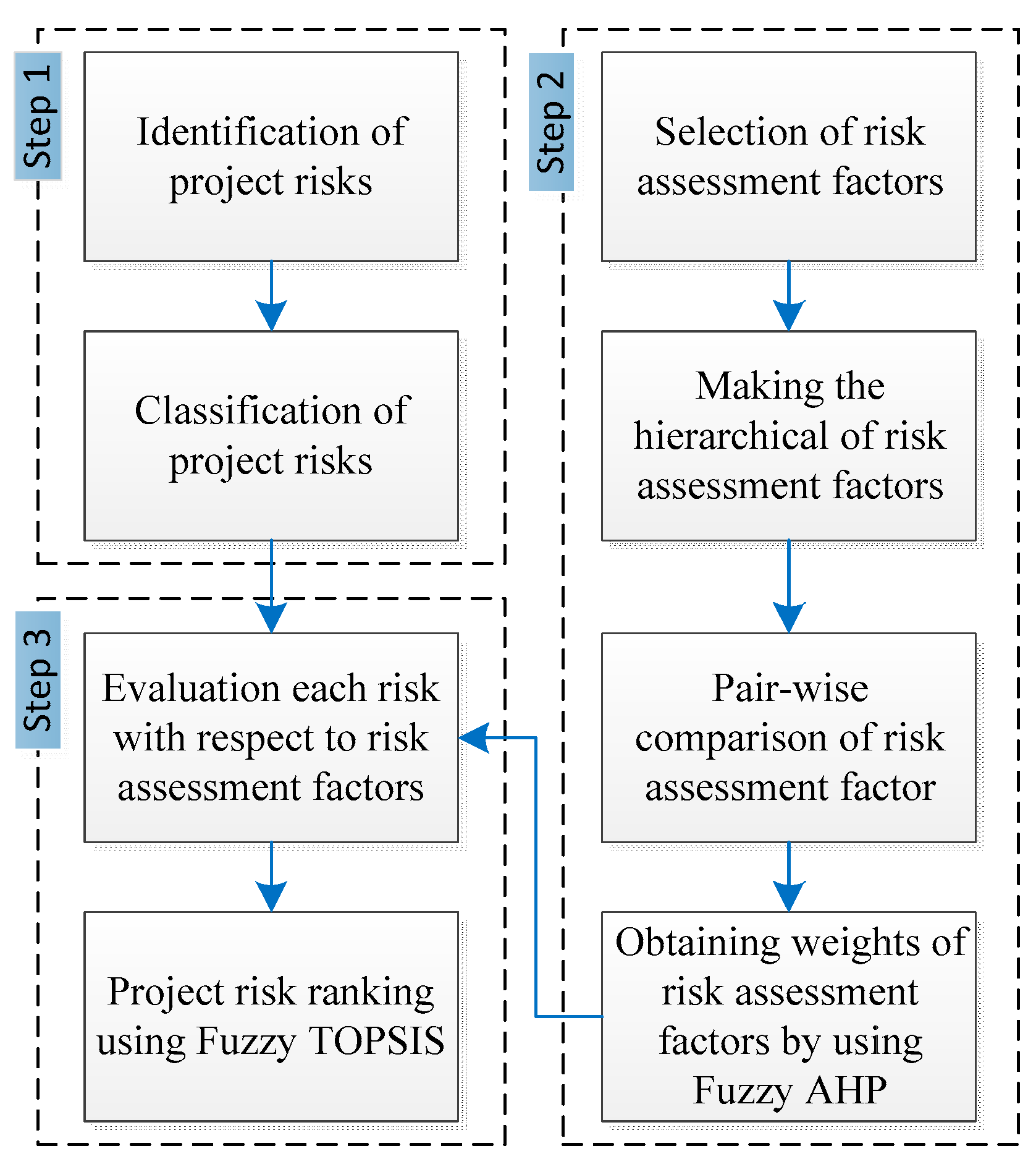
2. Materials and Methods

A modified fuzzy approach proposed by Kutlu and Ekmekçioğlu [63] is extended in this section for specifying the importance of the risks. In present study, risk assessment indicators in the traditional FMEA method are developed to determine the importance of risks. The domains of risk effectiveness on three principal criteria of cost, time and quality are broken down. Moreover, a corresponding weight is given to each risk assessment indicator. Because one factor of risk assessment is sometimes referred to other factors. For example, time may be preferred to cost in some projects. For this purpose, paired wise comparisons are used. The TOPSIS technique is used to rank the risks as per the assessment factors. So, the experts can express their judgment about any risk based on a precise number, a series of digital values, language phrases or fuzzy numbers. In a lot of situations, due to the quantitative uncertainty or non-measurability of the indicators, providing numerical values is difficult by the experts. Therefore, one can use a language variable or a fuzzy number. Due to the complexity of the largest projects and the lack of sufficient information, the fuzzy approach’s use is more appropriate [84]. Therefore, all calculations are based on triangular fuzzy numbers about the risk ranking process in this research. Figure 1 represents the proposed hybrid FMEA model for agricultural projects risk management.

To achieve these goals, the following steps are taken to identify the most important investment risks. The tools used in the proposed model are also described in the next section.

Step 1: Identify and categorize the investment risks

Step 2: Obtaining the weight of the risk assessment factors using Chang’s fuzzy AHP

• Draw a hierarchical chart of risk assessment factors.
• Formation of a pair-wise matrix of risk assessment factors (S, O, and D) and sub-risk assessment factors (ST, SC, and SQ) using triangular fuzzy numbers.
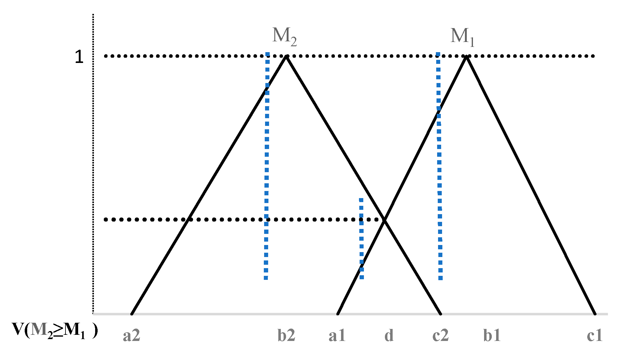
• Calculate Si for each of the two-dimensional matrix rows.
• Calculate the magnitude of Si’s relative to each other
• Calculate factors weight and risk factors under the paired matrix.
• Calculate the final weight vector at the lowest level of hierarchical structure.

Step 3: Risk rating using Chen’s fuzzy TOPSIS

• Assessing the experts with regards to the risks identified in each of the risk assessment factors.
• Create a fuzzy decision matrix and normalize it.
• Create a normal fuzzy decision matrix.
• Ideal positive ideal and adverse ideal fuzzy determination.
• Calculate the distance between all risks from a fuzzy positive and negative ideal
• Determine the proximity risk factor and calculate it.
• Risk rating according to their near-range ratio.

2.1. Fuzzy Logic

A good decision-making model must have effectiveness in inaccurate and vague conditions because vagueness is a prevalent feature of a lot of decision-making problems. Experts can make judgment according to an accurate numerical value, a range of numerical values, fuzzy numbers, and verbal phrases as well. There may sometimes be impossible to give numerical values due to uncertainty and the existence unmeasurable indices. Fuzzy number or verbal variable will therefore be used. It is better to apply the fuzzy approach in highly complex big projects and insufficient data [84]. Fuzzy set includes all the items groups each of which or their sub elements merit the property of membership function. A membership function varies between 0 and 1 meaning that there is a relative limited acceptability between the complete non-membership and complete dependency and this feature is relative, i.e., a boarder does not exist [85]. This theory is applied in ambiguous and uncertain conditions. This theory is capable of articulating many imprecise concepts and phrases in mathematics language and pave the path for reasoning, concluding, decision-making, and control in uncertain situations [86]. Despite the wide application of the fuzzy logic, its calculations are complicated generally. In the applied studies rectangular and triangular fuzzy numbers often are employed which can be performed easily for information processing and explaining results in the fuzzy conditions. In the current study, all the risks ranking calculations will be performed using the fuzzy triangular numbers.

In this method, the fuzzy numbers are demonstrated as 3 points (A = (a₁, a₂, a₃)) as shown in the Figure 2 adapted from [63]. The membership function is presented through Formula (1).

$${\mu }_A^{~}\left(x\right)=\left\{\begin{array}{cc}0,& x<a_1\\ \left(\frac{x-a_1}{a_2-a_1}\right),& a_1\le x\le a_2\\ \begin{array}{c}\left(\frac{a_3-x}{a_3-a_2}\right),\\ 0,\end{array}& \begin{array}{c}{a}_2\le x\le a_3\\ x>a_3\end{array}\end{array}\right\}$$

(1)

Having the triangular fuzzy number A = (a₁, a₂, a₃) and B = (b₁, b₂, b₃), the fuzzy operational rules of these fuzzy triangular numbers would be as follows [86]:

$$A (+) B=\left(a_1+b_1, a_2+b_2, a_3+b_3\right)$$

(2)

$$A(-)B=\left(a_1-b_1,a_2-b_2,a_3-b_3\right)$$

(3)

$$A(\times )B=\left(a_1\times b_1,a_2\times b_2,a_3\times b_3\right)$$

(4)

$$A(÷)B=\left(a_1÷b_3,a_2÷b_2,a_3÷b_1\right)$$

(5)

$$kA=\left(k{a}_1,k{a}_2,k{a}_3\right)$$

(6)

2.2. Fuzzy AHP

The analytic hierarchy process (AHP), that was developed by Saaty in 1980, is one of the most inclusive systems for multi-criteria decision making. It includes a pairwise comparison that facilitates judgments and calculations. In spite of the widespread application of the classical AHP in practical decision making problems, some criticized it for not handling adequately the uncertainty in mapping the perception of a decision maker to an exact number [87]. An optimal approach to deal with uncertain judgments is to express the ratio of the comparisons using fuzzy sets or numbers [88]. In the literature, several different methods and approaches have been proposed for “fuzzifying” AHP. Pedrycz and Laarhoven [89] performed studies that devised fuzzy logic principles to AHP. Buckley [90] implemented fuzzy numbers to demonstrate decision makers’ evaluation regarding various criteria of each decision. Chang [91] proposed an approach that can handle a pair-wise comparison instrument with triangular fuzzy numbers. Triantaphyllou [92] developed the multi-attribute decision making (MADM) fuzzy method. Their methodology was based on AHP method, coefficient model and TOPSIS method. Deng [87] introduced a simple fuzzy approach in order to solve qualitative multi-criteria problems. In the following, the concepts and definitions of fuzzy analytical hierarchy process will be presented based on the fuzzy triangular numbers and the extent analysis method [91]. Suppose M^j_gi is a triangular fuzzy number located at the row i and the column j in the pairwise comparisons matrix; then we have:

$${\displaystyle \sum }_{j=1}^m{M}_{gi}^j=\left({\displaystyle \sum }_{j=1}^m{a}_{ij},{\displaystyle \sum }_{j=1}^m{b}_{ij},{\displaystyle \sum }_{j=1}^m{c}_{ij}\right),i=1,2,3,\dots ,n$$

(7)

where c, b, a are the upper bound, mean and the lower bound of triangular fuzzy numbers respectively.

Fuzzy synthetic extent is shown by S_i and defined as:

$$S_i={\displaystyle \sum }_{j=1}^m{M}_{gi}^j\otimes {\left[{\displaystyle \sum }_{i=1}^n{\displaystyle \sum }_{j=1}^m{M}_{gi}^j\right]}^{-1}$$

(8)

To compute

$${\left[{\displaystyle \sum }_{i=1}^n{\displaystyle \sum }_{j=1}^m{M}_{gi}^j\right]}^{-1}$$

we act as follows:

$$\left[{\displaystyle \sum }_{i=1}^n{\displaystyle \sum }_{j=1}^m{M}_{gi}^j\right]=\left({\displaystyle \sum }_{i=1}^n{\displaystyle \sum }_{j=1}^m{a}_{ij},{\displaystyle \sum }_{i=1}^n{\displaystyle \sum }_{j=1}^m{b}_{ij},{\displaystyle \sum }_{i=1}^n{\displaystyle \sum }_{j=1}^m{c}_{ij}\right)$$

(9)

$${\left[{\displaystyle \sum }_{i=1}^n{\displaystyle \sum }_{j=1}^m{M}_{gi}^j\right]}^{-1}=\left(\frac{1}{{\sum }_{i=1}^n{\sum }_{j=1}^m{c}_{ij}},\frac{1}{{\sum }_{i=1}^n{\sum }_{j=1}^m{b}_{ij}},\frac{1}{{\sum }_{i=1}^n{\sum }_{j=1}^m{a}_{ij}}\right)$$

(10)

Then we have to determine the magnitude. For example, the magnitude of M₂ ≥ M₁ is as:

$$V\left(M_2\ge M_1\right)=Sup\left[min\left({\mu }_{M_1}\left(x\right),{\mu }_{M_2}\left(y\right)\right)\right],y\ge x$$

(11)

The magnitude is computed by the following formula:

$$V\left(M_2\ge M_1\right)=hgt\left(M_1{\displaystyle \cap }{M}_2\right)={\mu }_{M_2}\left(d\right)=\{\begin{array}{c} \begin{array}{cc}1,& IF{b}_2\ge b_1\end{array}\\ \begin{array}{cc}0,& IF{a}_1\ge c_2\end{array}\\ \begin{array}{cc}\frac{a_1-c_2}{(b_2-c_2)-(b_1-a_1)},& Otherwise\end{array}\end{array}$$

(12)

where d is the highest level between μ_M1 and μ_M2. Figure 3 adapted from [86] represents this concept.

In the next step, the magnitude of convex fuzzy numbers is defined as following:

$$V\left(M\ge M_1,M_2,\dots ,M_k\right)=V\left[\left(M\ge M_1\right)\&\dots \&\left(M\ge M_k\right)\right]=min\left(M\ge M_i\right)i=1,2,\dots ,K.$$

(13)

So we suppose that:

$$d^{\prime }\left(A_i\right)=minV\left(S_i\ge S_k\right).$$

(14)

The vector of weight is as:

$$W^{\prime }={\left(d^{\prime }\left(A_1\right),d^{\prime }\left(A_2\right),\dots ,d^{\prime }\left(A_n\right)\right)}^T.$$

(15)

After that we normalize the computed the weight vector:

$$W={\left(d\left(A_1\right),d\left(A_2\right),\dots ,d\left(A_n\right)\right)}^T.$$

(16)

In this way, we can calculate each sub-criterion weight.

In the current study, risk assessment factors in FMEA are performed by developing hierarchical structure of risk factors as shown in Figure 4. Base on reference [63] the continuum figured showed in

Table 1. Fuzzy spectrum for comparison of risk assessment factors.

Fuzzy Number	Description Term
(7,9,9)	Absolutely strong (AS)
(5,7,9)	Very strong (VS)
(3,5,7)	Fairly strong (FS)
(1,3,5)	Slightly strong (SS)
(1,1,1)	Equal (E)
(1/5,1/3,1)	Slightly weak (SW)
(1/7,1/5,1/3)	Fairly weak (FW)
(1/9,1/7,1/5)	Very weak (VW)
(1/9,1/9,1/7)	Absolutely weak (AW)

will be used for acquiring the ideas of the experts.

After achieving the pairwise comparison matrix, the consistency ration (CR) should be controlled. For this, the matrix can be defuzzified through graded mean integration and then calculate CR and get sure about its standardization. (CR ought to be less than 0.1). As per the graded mean integration we can convert a fuzzy number like $A=\left(a_1,a_2,a_3\right)$ to a crisp number through Equation (17) [63].

$$P\left(A\right)=\frac{a_1+4a_2+a_3}{6}$$

(17)

2.3. Fuzzy TOPSIS

TOPSIS is considered as a multi-criteria decision making model, which originally was introduced by Hwang and Yoon in 1981. Positive and negative ideal solutions are the principled logic of the method. The ideal positive solution maximizes the profit criteria while minimizes the criteria of cost [93]. TOPSIS method has been used with the fuzzy numbers too. Chen and Hwang used the fuzzy logic in TOPSIS first [94]. Fuzzy TOPSIS method is suitable to solve the problems in fuzzy multi-attribute group decision making. For example, fuzzy TOPSIS has been used in selecting plant location [95], supplier selection [96], green supplier selection in agri-supply chain industry [97] Industrial robotic system selection [98], best energy technology selection [93], consumer’s product adoption modelling [99] and project selection based on risk [64]. Also, Kutlu and Ekmekçioğlu [63] proposed a hybrid approach on FAHP and FTOPSIS methods for ranking the potential failure modes in a design, a manufacturing, or service. Chen’s fuzzy TOPSIS method [100] is explained here. Suppose we have m alternatives, k decision-makers, and n criteria. Multi-criteria fuzzy group decision-making (MCDM) problem can easily be expressed in a matrix format as following:

$$D=\begin{array}{c}\begin{array}{ccc}{C}_1& \begin{array}{ccc}\dots & C_j& \dots \end{array}& C_n\end{array}\\ \begin{array}{c}{A}_1\\ ⋮\\ \begin{array}{c}{A}_i\\ ⋮\\ A_m\end{array}\end{array}\left[\begin{array}{ccc}{x}_{11}& \begin{array}{ccc}\dots & x_{1j}& \dots \end{array}& x_{1n}\\ ⋮& ⋮& ⋮\\ \begin{array}{c}{x}_{i1}\\ ⋮\\ x_{m1}\end{array}& \begin{array}{c}\begin{array}{ccc}\dots & x_{ij}& \dots \end{array}\\ ⋮\\ \begin{array}{ccc}\dots & x_{mj}& \dots \end{array}\end{array}& \begin{array}{c}{x}_{in}\\ ⋮\\ x_{mn}\end{array}\end{array}\right]\end{array}i=1,2,\dots ,m;j=1,2,\dots ,n.$$

(18)

Here, A₁, A₂…, A_n are the alternatives which should be selected or prioritized. C₁, C₂,…, C_n are characteristics or criteria of assessment. X_i1, X_ij,…, X_in are the A_i alternative rating respect to criterion or characteristics C₁, C₂,…, C_n evaluated by K. Average value method is applied to integrate fuzzy scores of performance of evaluator K.

$$x_{ij}=\frac{1}{k}\left[x_{ij}^1(+)x_{ij}^2(+)\dots (+)x_{ij}^k\right]$$

(19)

where X_ij is the alternative A_i rating respect to criterion C_j when evaluated by K.

In combining experts’ opinions (combining fuzzy numbers), we can use the minimum number of experts’ opinions for lower bound, the maximum number of experts’ opinions for upper bound and the average number of experts’ opinions for middle numbers. Then, we can get the fuzzy normalized decision matrix defined by $R.$

$$R={\left[r_{ij}\right]}_{m\times n}i=1,2,\dots ,m;j=1,2,\dots ,n$$

(20)

The following formulas are used to normalize the fuzzy decision matrix in terms of the criteria of benefit (B) and cost (C).

$$r=\left(\frac{a_{ij}}{c_j^{*}},\frac{b_{ij}}{c_j^{*}},\frac{c_{ij}}{c_j^{*}}\right),jϵB;$$

(21)

$$r=\left(\frac{a_j^{-}}{c_{ij}},\frac{a_j^{-}}{b_{ij}},\frac{a_j^{-}}{a_{ij}}\right),jϵC;$$

(22)

$$c_j^{*}={max}_i{c}_{ij}ifj\in B;$$

(23)

$$a_j^{-}={min}_i{a}_{ij}ifj\in C;.$$

(24)

Then the normalized weighted decision matrix V is achieved by multiplying the weight of importance (w_j) of the criteria of evaluation with the normalized fuzzy decision matrix r_ij.

The normalized weighted fuzzy decision matrix V is defined as below:

$$V={\left[v_{ij}\right]}_{m\times n},i=1,2,\dots ,m;j=1,2,\dots ,n,$$

(25)

$$v_{ij}=r_{ij}\otimes w_j.$$

(26)

In which the fuzzy number W is the criterion j weight. Because the triangular positive fuzzy numbers are in the interval [0,1], hence the positive-ideal fuzzy solution and negative-ideal fuzzy solution, can be defined as follows.

$$A^{*}=\left(v_1^{*},v_2^{*},\dots ,v_n^{*}\right),$$

(27)

$$A^{-}=\left(v_1^{-},v_2^{-},\dots ,v_n^{-}\right),$$

(28)

$$v_j^{*}=\left(1,1,1\right)and{v}_j^{-}=\left(0,0,0\right),j=1,2,\dots ,n.$$

(29)

Then the distance of each alternative from $A^{*}$ and $A^{-}$ can be computed as

$$d_i^{*}={\displaystyle \sum }_{j=1}^{n}d\left(v_{ij},v_j^{*}\right),i=1,2,\dots ,m.$$

(30)

$$d_i^{-}={\displaystyle \sum }_{j=1}^{n}d\left(v_{ij},v_j^{-}\right),i=1,2,\dots ,m.$$

(31)

where d is the distance of the one fuzzy number from the other that can be calculated for example with the formula as follows.

$$d\left(v_{ij},v_j^{*}\right)=\sqrt{\frac{1}{3}\left[{\left(a-1\right)}^2+{\left(b-1\right)}^2+{\left(c-1\right)}^2\right]}$$

(32)

$$d\left(v_{ij},v_j^{-}\right)=\sqrt{\frac{1}{3}\left[{\left(a-0\right)}^2+{\left(b-0\right)}^2+{\left(c-0\right)}^2\right]}.$$

(33)

When the coefficient of closeness was determined, one can obtain the rank order of all alternatives, so allow the decision-makers to select the alternative with the most feasibility. The coefficient of closeness for each alternative can be calculated as follows.

$$C{C}_i=\frac{d_i^{-}}{d_i^{*}+d_i^{-}},i=1,2,\dots ,m.$$

(34)

Thus, the options are listed in CC_i descending order. In creating a decision matrix, each identified risk is assessed for its probability of occurrence, severity and their potential impact on objectives of project in terms of time, quality and cost. This is achieved by designing different methods and questionnaires and obtaining data from experts. In this research, Abdelgawad and Fayek [23] studies are used to achieve experts’ judgment. The combination of linguistic terms and triangular fuzzy numbers is based on the

Table 2. Linguistic definition of probability of occurrence, severity, and detection.

Fuzzy Number	Description Term	Probability of Occurrence	Severity On			Detection/Control
			Cost	Time	Quality
(1,1,3)	Very low (VL)	Chance is < 1%	Increased costs < 1%	Increased time < 1%	Quality degradation is not noticeable.	Not capable of detecting and controlling the risk event
(1,3,5)	Low (L)	Chance is ≥ 1% and < 10%	≥1% and<4%	≥1% and <4%	Few areas of quality are affected.	Low chance of detecting and controlling the risk event
(3,5,7)	Moderate (M)	Chance is ≥ 10% and < 33%	≥4% and <7%	≥4% and <7%	Major areas of quality are affected.	Moderate chance of detecting and controlling the risk event
(5,7,9)	High (H)	Chance is ≥ 33% and < 67%	≥7% and <10%	≥7% and <10%	Quality are unacceptable to project sponsor.	High chance of detecting and controlling the risk event
(7,9,9)	Very high (VH)	Chance is ≥ 67%	≥10%	≥10%	Project quality does not meet business expectations.	High effectiveness in detecting and controlling the risk event

.

2.4. Identification and Classification of Investment Risks

In this section, the introduced methodology of risk assessment is used in five agricultural projects, including citrus gardens, pistachio gardens, olive groves, and black and green gardens named P1 to P5 respectively. The location of projects is taken place in various cities of Iran with different climatic conditions. Naturally, due to different parameters such as the target market, the financing of the project, the specialized knowledge required, and the other, each project’s risk conditions will be different. Investors are demanding risk analysis from the start of the project until the first harvest. According to Hillson [101], risk management is the first step in identifying and categorizing risks, regardless of the risk assessment technique. Therefore, before using the proposed method, it is required to know the agricultural field’s risk. In the field of agricultural risk literature, one can introduce five risks including risk of production, credit risk, human risk, market risk and environment risk. Meanwhile Hardaker [9] extends these risks by including business and political risks to the above cases. Girdzuite divides the agricultural risks to five risks: Human, production, political, economic and credit. Leherner defines the agricultural risks as follows.

Market and price risk, production facility risk, financial risk, human resource risk, production risk, political risks, other risks such as environment risks and burglary [7]. Based on Miller and co-authors one can classify risk in agriculture into: Production risk that was caused by weather fluctuations, crop diseases and pests, price risk that was caused by price volatility, disaster risk (e.g., floods, hurricanes, droughts, etc.) and technological risk that was resulting from continuous development and adaptation of new methods and techniques in production [8]. Another agricultural risk classification is based on the study of the European Commission: Personal (e.g., health loss and living by people who work on the farm), institutional (e.g., trade regulations, political), financial (e.g., loans access and the crediting conditions stability), production (causes of the phenomena are because of climate conditions, thefts, pests, fires) and price (i.e., unfavorable changes in prices in the market of agricultural products and production factors) [6]. After identifying the risks, the risks should be classified and structured. The structure of risk breakdown is a hierarchical structure of research risks, used to organize and direct the risk management process [102]. According to the PMBOK standard, project risks contain four groups: External, inter-organizational, technical-, qualitative-, functional-, and project management risk. The risk can be calculated conditionally for each phase and then a general risk obtained from the combination of these risks. As per to Meredith et al. [103], there are two important risk classes: Technical risk and business risk. The technical risk poses the probability that a product cannot fully develop in the development process, and the business risk is the probability of a product or service market failure in the target market, assuming that the product or service has been well developed and developed.

In this research, according to the literature review and with the help of a group of agricultural experts, 10 investment risks are identified in 5 agricultural projects and are divided into two phases of construction and operation. According to this categorization, risk analysis can be done in two phases of operation and construction. 10 The risk identified by the R1 to R10 codes are demonstrated in

Table 3. Identification and categorization of investment risks.

Risk Category	ID	Type of Risk
Construction risks	R1	Risk of project manager and human resources
	R2	Risk of project planning and implementation
	R3	Financial risk
	R4	Risk of increasing costs
	R5	The risk of access to technology and knowledge
Operational risks	R6	The supply of raw materials (fluctuations in the prices of agricultural raw materials, including seeds, fertilizers, etc.)
	R7	Risk energy and water resources
	R8	The risk of climate fluctuations and pests
	R9	Marketing and sales risk at home and abroad
	R10	Limitations on product sales price (due to government regulations, competitive market, etc.)

Source: Authors’ elaboration.

.

2.5. Investment Risk Assessment

After determining and categorizing investment risks, the importance of the factors at the lowest level must be considered according to the hierarchical structure of factors of assessing risk (ST, SC, SQ, O, and D). For this purpose, by designing a paired comparison questionnaire, three groups of three experts are asked to compare each of the main factors of risk (S, D, and O) in relation to agricultural projects and make their views known. The integration of expert opinions is done using the geometric mean. Comments 3 Expert groups and summary of results are evident in

Table 4. Evaluation of experts in the first level of risk assessment factors.

	S	O	D	Weight Vector
Severity (S)		SS- SS –FW (0.52, 1.22, 2.03)	FS-VS-SW (1.44, 2.27, 3.98)	0.425
Occurrence (O)			SS-SS-E (1, 2.08, 2.92)	0.390
Detection (D)				0.185

CR for defuzzified type of this matrix 0.00017< 0.10.

.

In calculations, according to the AHP process, $\sum _{\mathrm{j}=1}^{\mathrm{n}}{\mathrm{M}}_{\mathrm{gi}}^{\mathrm{j}}$ for the first row of the matrix is computed as follows.

C₁: (1+ 0.52+ 1.44, 1+ 1.22+ 2.27, 1+ 2.03+ 3.98) = (2.97, 4.48, 7.00).

Similarly, for other rows C₂ and C₃ can be obtained as follows.

C₂ = (2.49, 3.90, 5.83)

C₃ = (1.59, 1.92, 2.69).

Therefore, following results can be derived.

$${\sum }_{i=1}^n{\sum }_{j=1}^m{M}_{gi}^j=(2.97+2.49+1.59,4.48+3.90+1.92,7.00+5.83+2.69)=(7.05,10.30,15.53)$$

$${\left[{\sum }_{i=1}^n{\sum }_{j=1}^m{M}_{gi}^j\right]}^{-1}=(0.064,0.097,\mathrm{and}0.141).$$

${\mathrm{S}}_{\mathrm{i}}$ for each row of the pairwise comparisons matrix is calculated as:

$$S_i= {\displaystyle \sum }_{j=1}^m{M}_{g_i}^j \times {\left[{\displaystyle \sum }_{i=1}^n{\displaystyle \sum }_{j=1}^m{M}_{g_i}^j\right]}^{-1}$$

S₁: (2.97, 4.48, 7.00) ⊗ (0.064, 0.097, 0.141) = (0.19, 0.43, 0.99)

S₂: (2.49, 3.90, 5.83) ⊗ (0.064, 0.097, 0.141) = (0.16, 0.37, 0.82)

S₃: (1.59, 1.92, 2.69) ⊗ (0.064, 0.097, 0.141) = (0.10, 0.18, 0.38).

The degrees of each of the $S_i$ related to each other can be represented as follows.

$$\mathrm{V}(\mathrm{S}1\ge \mathrm{S}2)=1\mathrm{V}(\mathrm{S}1\ge \mathrm{S}3)=1\min \left\{\mathrm{V}\right(S_i\ge S_k\left)\right\}=1$$

$$\mathrm{V}(\mathrm{S}2\ge \mathrm{S}1)=0.92\mathrm{V}(\mathrm{S}2\ge \mathrm{S}3)=1\min \left\{\mathrm{V}\right(S_i\ge S_k\left)\right\}=0.92$$

$$\mathrm{V}(\mathrm{S}3\ge \mathrm{S}1)=0.43\mathrm{V}(\mathrm{S}3\ge \mathrm{S}2)=0.54\min \left\{\mathrm{V}\right(S_i\ge S_k\left)\right\}=0.43.$$

Therefore, the unweighted weight (1, 0.92, 0.43) and the normalized weight are calculated as (0.42, 0.39, 0.18).

Table 5. Evaluation of experts in second level of risk assessment factors.

	ST	SC	SQ	Weight Vector
Severity on Time (ST)		FW-SS-SW (0.31, 0.58, 1.19)	E-SS-E (1, 1.44, 1.71)	0.309
Severity on Cost (SC)			FS-E-SS (1.44, 2.47, 3.27)	0.532
Severity on Quality (SQ)				0.159

CR for defuzzified type of this matrix 0.00031 < 0.10

demonstrates the results of paired comparisons at the second level of hierarchical structure or risk severity assessment factors (ST, SC, and SQ). Finally, the final weights of each of the risk assessment factors for time, cost, quality, probability and detection and control are respectively 0.131, 0.226, 0.068, 0.390, and 0.185, respectively, according to

Table 6. Final weight vector.

Occurrence	Severity			Detection
0.390	0.425			0.185
	Severity on Time	Severity on Cost	Severity on Quality
	0.309	0.532	0.159
	0.131	0.226	0.068

.

Subsequently, the projects are evaluated using five risk assessment factors in each of the risks. To this end, by designing a questionnaire in accordance with the spectrum of the Table 2, the experts’ opinions about the likelihood of occurrence, the severity of the cost, the time and quality, and the ability to discover and control each risk identified in each project are received.

Table 7. Evaluation of experts in linguistic variables for risks in first project.

Category	Risks	O	ST	SC	SQ	D
		Max	Max	Max	Max	Min
		0.390	0.131	0.226	0.068	0.185
Construction risks	R1	M-L-L	H-VH-L	L-VL-L	VL-VL-L	H-M-M
	R2	H-H-M	H-H-M	H-M-M	L-L-M	H-VH-H
	R3	H-H-VH	H-M-H	VL-L-L	VL-VLVL	M-L-L
	R4	M-M-H	M-VL-L	VH-VH-VH	M-H-M	VL-VL-L
	R5	VL-L-VL	VL-VL-VL	M-L-M	L-M-M	L-L-L
Operational risks	R6	M-M-L	VH-VH-H	VH-VH-H	VH-VH-VH	M-L-L
	R7	VH-H-VH	M-M-L	VH-H-VH	VH-VH-VH	L-VL-L
	R8	VH-H-VH	L-L-M	M-H-M	VH-VH-VH	M-VL-L
	R9	M-L-M	VL-VL-VL	M-L-M	VL-VL-VL	M-H-H
	R10	H-VH-VH	VL-VL-VL	H-H-M	VL-VL-L	L-VL-L

(VL = Very low, L = Low, M = Moderate, H = High, VH = Very high)

shows the views of three groups of experts on each of the risk assessment factors in relation to the first project. For example, experts rated the probability of occurrence (O) of the first risk (R1) as Moderate (M), LOW (L), and LOW (V) respectively. The severity of the first risk (R1) on the project time (ST), will be High (H), Very High (VH), and LOW (V), respectively. Regarding the nature of the indices, it can be said that the probability risk index, the severity of the cost, the time, and the quality are of a positive nature, the higher the amount, the higher the risk, but in the case of the index of evaluation of the discovery and control of the theorem the above is the reverse. That is, the higher the ability to detect and control the risk, the lower the risk.

Table 8. Integrating the expert opinions.

Risk ID	O	ST	SC	SQ	D
R1	1, 3.7, 7	1, 6.3, 9	1, 2.3, 5	1, 1.7, 5	3, 5.67, 9
R2	3, 6.3, 9	3, 6.3, 9	3, 5.7, 9	1, 2.3, 7	5, 7.67, 9
R3	5, 7.7, 9	3, 6.3, 9	1, 2.3, 5	1, 1, 3	1, 3.67, 7
R4	3, 5.7, 9	1, 3, 7	7, 9, 9	3, 5.7, 9	1, 1.67, 5
R5	1, 1.7, 5	1, 1, 3	1, 4.3, 7	1, 4.3, 7	1, 3, 5
R6	1, 4.3, 7	5, 8.3, 9	5, 8.3, 9	7, 9, 9	1, 3.67, 7
R7	5, 8.3, 9	1, 4.3, 7	5, 8.3, 9	7, 9, 9	1, 2.33, 5
R8	5, 8.3, 9	1, 3.7, 7	3, 5.7, 9	7, 9, 9	1, 3, 7
R9	1, 4.3, 7	1, 1, 3	1, 4.3, 7	1, 1, 3	3, 6.33, 9
R10	5, 8.3, 9	1, 1, 3	3, 6.3, 9	1, 1.7, 5	1, 2.33, 5

shows the integration of expert opinions. In compiling the opinion of the experts (fuzzy number combination), the experts’ opinions are used for maximum. For the average numbers, also the average of experts’ opinion is used. According to the calculations of the FTOPSIS method, the non-equilibrium matrix obtained is shown in

Table 9. The non-equilibrium matrix and calculating the closeness coefficient.

Risk ID	O	ST	SC	SQ	D	${\mathit{d}}_{\mathit{i}}^{*}$	${\mathit{d}}_{\mathit{i}}^{-}$	$\mathit{C}{\mathit{C}}_{\mathit{i}}$- Score	Rank
R1	0.04, 0.16, 0.30	0.01, 0.09, 0.13	0.03, 0.06, 0.13	0.01, 0.01, 0.04	0.02, 0.03, 0.06	0.39	0.20	0.340	8
R2	0.13, 0.27, 0.39	0.04, 0.09, 0.13	0.08, 0.14, 0.23	0.01, 0.02, 0.05	0.02, 0.02, 0.04	0.30	0.29	0.490	7
R3	0.22, 0.33, 0.39	0.04, 0.09, 0.13	0.03, 0.06, 0.13	0.01, 0.01, 0.02	0.03, 0.05, 0.19	0.29	0.30	0.514	6
R4	0.13, 0.25, 0.39	0.01, 0.04, 0.10	0.18, 0.23, 0.23	0.02, 0.04, 0.07	0.04, 0.11, 0.19	0.24	0.36	0.603	3
R5	0.04, 0.07, 0.22	0.01, 0.01, 0.04	0.03, 0.11, 0.18	0.01, 0.03, 0.05	0.04, 0.06, 0.19	0.4	0.2	0.335	9
R6	0.04, 0.19, 0.30	0.07, 0.12, 0.13	0.13, 0.21, 0.23	0.05, 0.07, 0.07	0.03, 0.05, 0.19	0.26	0.34	0.562	4
R7	0.22, 0.36, 0.39	0.01, 0.06, 0.10	0.13, 0.21, 0.23	0.05, 0.07, 0.07	0.04, 0.08, 0.19	0.2	0.39	0.655	1
R8	0.22, 0.36, 0.39	0.01, 0.05, 0.10	0.08, 0.14, 0.23	0.05, 0.07, 0.07	0.03, 0.06, 0.19	0.24	0.37	0.609	2
R9	0.04, 0.19, 0.30	0.01, 0.01, 0.04	0.03, 0.11, 0.18	0.01, 0.01, 0.02	0.02, 0.03, 0.06	0.40	0.19	0.319	10
R10	0.22, 0.36, 0.39	0.01, 0.01, 0.04	0.08, 0.16, 0.23	0.01, 0.01, 0.04	0.04, 0.08, 0.19	0.27	0.33	0.552	5
$A^{*}$	0.39	0.13	0.23	0.07	0.19
$A^{-}$	0.04	0.01	0.03	0.01	0.02

Source: Authors’ elaboration.

, where the positive and the negative ideals are represented. It also shows the distance from the positive ideal and negative ideal, based on which the score or the coefficient of closeness of each risk is calculated. On this basis, each risk is ranked in the first project. As is clear, the most significant risk in the first project is risk 7, which is the risk of supply of energy and water resources.

This ranking is also done for four other agricultural projects. In Appendix A (

Table A1. Comments from three groups of experts for each of the projects.

Project	ID	Probability	Severity			Discover and Control
		P	(Time) ST	(cost) SC	(Quality) SQ	D
The second project	R1	L-L-M	L-VL-VL	M-M-M	VL-VL-VL	M-M-H
	R2	L-L-VL	VL-VL-VL	L-L-M	L-M-M	L-L-M
	R3	M-M-M	M-VL-L	VH-L-VH	H-L-L	VL-VL-L
	R4	H-H-M	L-M-H	VH-VH-VH	M-VL-VL	M-L-L
	R5	M-L-L	L-L-L	L-VL-L	VL-VL-L	H-H-M
	R6	M-H-M	L-M-L	VH-H-VH	VH-VH-VH	L-VL-L
	R7	H –H- M	M-M-M	VH-VH-H	VH-VH-VH	H-L-L
	R8	VH-VH-H	L-L-M	VH-H-M	VH-VH-VH	M-VL-L
	R9	VL-L-M	VL-L-M	L-M-M	VL-L-VL	H-VH-H
	R10	H-M-VH	VL-VL-VL	L-H-M	VL-VL-L	L-VL-M
The third project	R1	H-M-L	VH-H-H	VH-H-H	H-VH-L	H-M-L
	R2	H-M-VH	H-VH-M	VH-H-M	H-H-M	H-VH-H
	R3	H-H-H	H-VLVL	L-H-L	L-VL-M	M-L-L
	R4	VH-VH-H	L-H-M	VH-M-H	L-VL-L	VL-VL-VL
	R5	VH-H-VH	L-M-M	VH-H-VH	H-M-H	M-L-L
	R6	H-H-M	M-M-M	M-M-VH	VH-VH-H	M-L-L
	R7	VH-H-VH	H-M-M	VH-H-VH	VH-VH-H	L-VL-M
	R8	M-H-VH	VH-H-H	VH-VH-VH	VH-VH-VH	M-VL-L
	R9	M-H-M	L-VL-L	M-H-M	L-VL-VL	M-VL-VL
	R10	H-H-VH	L-VL-L	H-VH-VH	VL-VL-VL	M-M-L
The fourth project	R1	L-VL-L	VH-H-H	L-M-M	H-VH-H	L-M-L
	R2	L-VL-H	VH-VH-M	H-H-M	H-H-VH	M-M-H
	R3	L-VL-L	H-M-M	H-H-VH	L-VL-L	M-H-L
	R4	H-VH-H	L-L-L	VH-VH-H	H-M-L	L-VL-L
	R5	M-H-M	L-M-L	M-M-M	M-M-H	M-L-L
	R6	M-H-M	L-L-M	H-M-VH	VH-VH-H	M-L-L
	R7	H-H-VH	L-L-M	H-H-H	VH-VH-H	L-VL-M
	R8	H-H-VH	VH-H-H	VH-VH-VH	VH-VH-VH	L-VL-L
	R9	M-H-M	VL-VL-VL	VH-H-M	VL-VL-VL	L-VL-VL
	R10	VH-H-VH	VL-VL-L	H-VH-VH	VL-VL-VL	VL-M-L
The fifth project	R1	L-M-L	VH-H-H	H-M-M	VH-VH-H	L-M-L
	R2	L-VL-M	VH-VH-H	H-H-VH	H-M-VH	M-M-H
	R3	H-VH-H	H-VH-H	H-H-VH	L-VL-L	M-M-L
	R4	VH-VH-H	L-L-L	VH-VH-H	H-M-H	L-VL-L
	R5	VL-L-VL	VL-M-L	L-M-L	L-M-L	M-H-VH
	R6	M-M-M	M-L-M	H-M-VH	H-VH-H	M-H-H
	R7	M-H-M	L-L-M	H-H-H	VH-VH-VH	H-M-M
	R8	L-M-M	VH-H-H	VH-VH-VH	VH-VH-VH	L-VL-L
	R9	L-M-M	VL-VL-VL	VH-H-M	VL-VL-VL	L-VL-VL
	R10	H-H-VH	VL-VL-L	H-VH-VH	VL-VL-VL	M-M-L

), the information for these four projects is presented. In this section, only the calculation results are presented in

Table 10. The results of fuzzy technique for order of preference by similarity to ideal solution (FTOPSIS) output and ranking the risks in 5 investment projects.

Risk ID	Project 1		Project 2		Project 3		Project 4		Project 5
	Score	Rank	Score	Rank	Score	Rank	Score	Rank	Score	Rank
R1	0.340	8	0.342	7	0.584	5	0.429	10	0.511	6
R2	0.490	7	0.333	8	0.524	8	0.482	8	0.481	7
R3	0.514	6	0.502	5	0.506	9	0.445	9	0.592	3
R4	0.603	3	0.592	3	0.601	4	0.610	3	0.624	1
R5	0.335	9	0.304	10	0.639	3	0.512	6	0.299	10
R6	0.562	4	0.591	4	0.579	6	0.548	5	0.470	8
R7	0.655	1	0.599	2	0.671	2	0.700	2	0.583	4
R8	0.609	2	0.617	1	0.712	1	0.716	1	0.594	2
R9	0.319	10	0.330	9	0.500	10	0.498	7	0.436	9
R10	0.552	5	0.487	6	0.568	7	0.582	4	0.573	5

. As is evident, the important risks are: Risk 7 in the first project (supply of water resources and energy), risk 8 in the second, third and fourth projects (weather and pest control) and risk 4 in the fifth project (increase of costs).

3. Results and Discussion

According to the results of various risks in different projects, they have a different rating and ranking. This can be caused by differences in investment positions such as geographic location, climate, investment conditions, number of specialists in the region and etc. Comparing the risk rating for different projects and the status of the ten risks in each investment project are shown in Figure 5 and Figure 6. In case of implementation of any project, risk-taking measures should be taken in order of importance. As it is known, the most important risks in the projects are risks 7 and 8, namely the risk of water and energy supplies, and the risk of climate fluctuations and pests, which is well understood in agriculture.

A sensitivity analysis is done by weighting the risk assessment factors as per the information given in

Table 11. Risk assessment factors weights regarding the considered statuses.

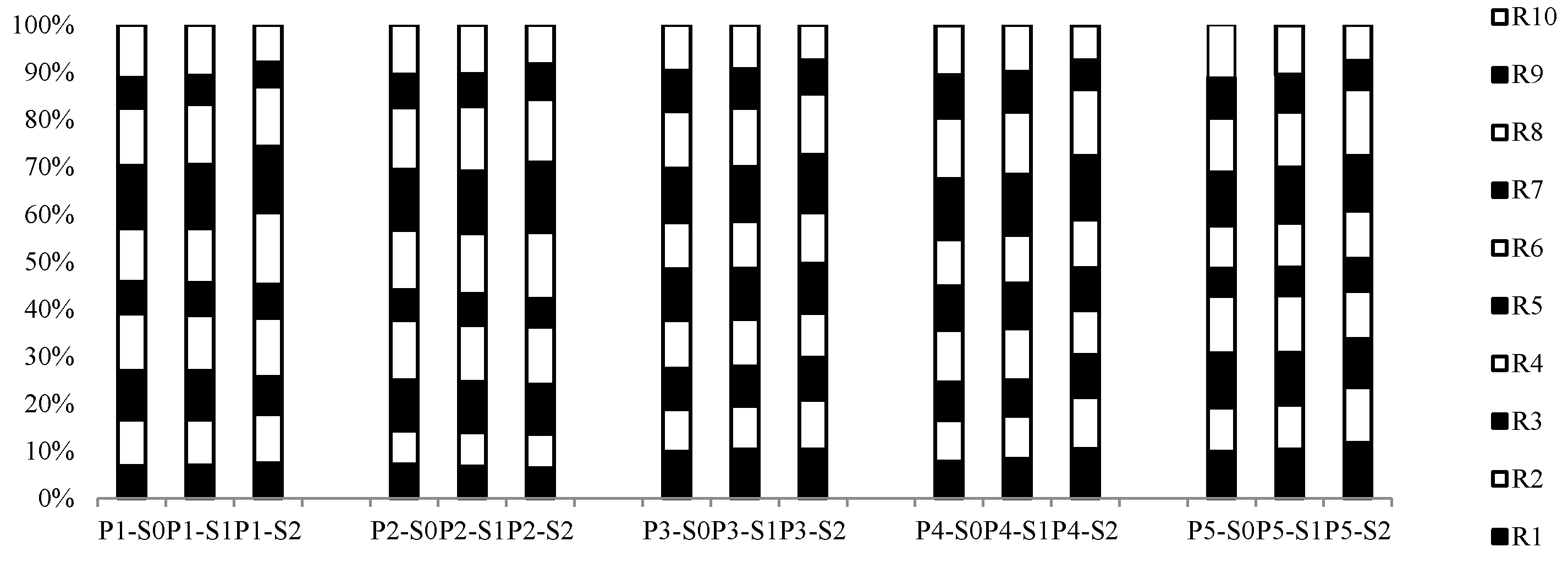
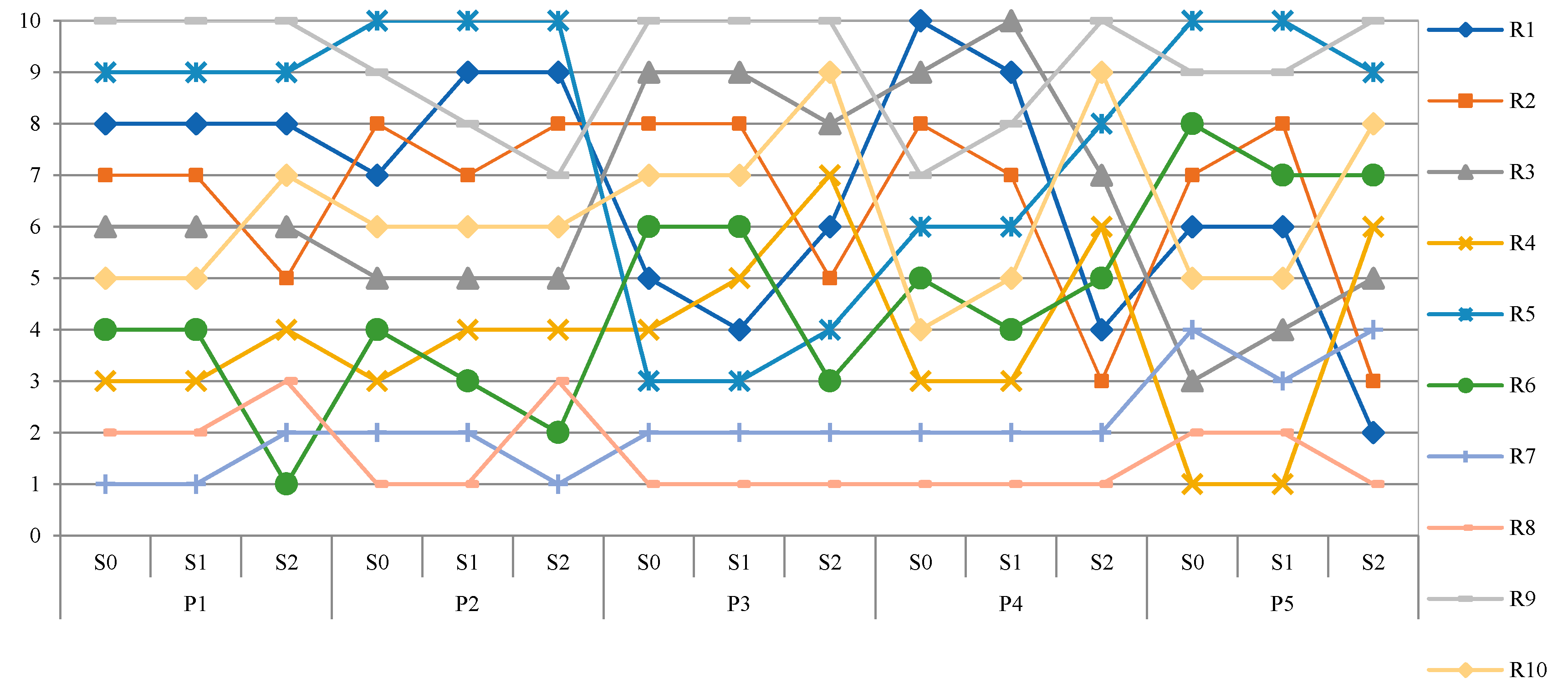
Factors of Risk Assessment	Status 0 (S0)	Status 1 (S1)	Status 2 (S2)
O	0.390	0.390	0.300
ST	0.131	0.141	1.333
SC	0.226	0.141	1.333
SQ	0.068	0.141	1.333
D	0.185	0.185	0.300

. The given information describes the weight of the risk assessment factors in the original situation and the first and second situation. Figure 7 and Figure 8 show the results of these changes in percentage and risk ranking in each investment project.

The results show that the risk weighting factors changed the risk priority between the different projects by affecting the weights. For example, the most important risk in the first project is in Status 0 and 1 is risk 7, but in status 2 it is risk 6. Similarly, in the case of the second project, the most significant risk in Status 0 and Status 1 is risk 8 and in Status 2 it is risk 7 and so on. In order to rank all the risks in a general way (considering all the projects), the risk rating can be averaged in different projects. This is done in three modes: Original, first, and second situation. Figure 9 shows the results of this type of ranking. Different colors represent the risks of building phase and the risks of exploitation phase.

Controlling the Risks in the Agricultural Sector

Identification and evaluation of risks would not be useful without regarding them. Risk control strategies in the agricultural sector can be divided into two groups according to the European Commission [6] as follows.

• On-farm strategies including: Selection of low risk exposure products, selection of short production cycles products, production programs diversification, and self-insurance or stabilization funds.
• Strategies of risk-sharing including: Marketing and production contracts, futures markets hedging, or the participating in insurance, mutual insurance or mutual regional schemes.

According to Hillson [102], a common risk response category is four of the avoidance, reduction, transfer, and acceptance of risk, where risk control issues in agriculture can be grouped into these four categories. For example, in risk mitigation techniques the techniques used generally reduce risk. Farmers traditionally apply some methods such as horizontal variation, vertical diversity, cultivation, and the use of robust, but low-yielding products to reduce the risks of agriculture. A wealthy company can accumulate wealth or benefits in years of good to protect itself in bad years. It actually distributes risk over time. It can also diversify the cultivation in different parts of the earth or in different products, that is, to distribute risk at the location. Another way of dealing with risk is transferring risk. The most common methods of transferring risk in agriculture include collective cultivation, use of futures markets, pre-sale contracts, guaranteed prices, and insurance.

In this research, the risk of fluctuation of climate and air (R8) is the most important risk in agricultural projects. In this regard, agricultural insurance can be considered. Another issue that should be considered by government institutions is the strong production of the import market and the prevention of dumping by foreign commodities which have received subsidies on the origin market and make the domestic market sometimes get out of profit. For this purpose, revenue insurance and the guarantee of purchase are covered, which covers market losses. Therefore, it could reduce the risk of selling price limits (R10). Lack of channels for proper marketing, forces the farmers to distress sale which will result in income reduction to the farmers and benefit the middlemen [104]. In the area of product marketing and marketing risk at home and abroad (R9), an appropriate risk mitigation strategy can be horizontal integration. In this case, the yield produced by the farmers should be considered as an input in the other fields, since the dependence on the domestic and foreign markets is reduced. Consequently, the possible constraints do not give rise to any significant damage. Therefore, another issue is the completion of supply chain and the double importance of the food and processing industries, which, along with marketing, can push the sector into profitability as much as possible. Supply chain in agriculture is comparable highly with a production-focused system, incorporating the planting, breed, process, producing, transporting, and delivery activities [105].

Some other common methods used by agricultural producers to manage risk can be the use of diversification in products and activities (R10 and R9 risk reduction), optimal allocation of credit resources to the financial needs of activities (R3 risk reduction), pre-sales of the produce (Reducing risk R10 and R9), creating a fence against the price by selling the produce through future contracts or option contracts (R10 risk reduction), creating diversification of assets and turning them into assets with the ability to quickly convert to liquidity, and finally leaving the agricultural activities. In general, the fluctuation in agricultural incomes and probability of losses for producers in most of the less developed countries and even in a lot of developing countries are uncontrollable factors, and risks that are not controlled by risk management methods can be considered by the government. They are required to prepare programs to stabilize producers’ revenues, such as compensatory payments, determination of guaranteed prices, targets, and purchases of credit or insurance for agricultural products [6]. Additionally, in agriculture sector to achieve a sustainable development, management view is not be restricted to agricultural production but should cover the supply chain entirely [97,106]. Problems such as lack of insufficient participation of local farmers, lack of strong control of food safety and quality [107], traditional methods, and poor management [108] have been identified as the constrains of sustainable supply chain performance [109,110].

4. Conclusions

FMEA is a technique used in reliability programs. This technique can provide the required information for risk management decisions. Although this technique is used more in the field of process and production, its application is also seen in evaluating the projects risk. In the traditional FMEA, the ranking of critical failure states is performed using criteria such as the probability of occurrence (O), detection (D), and severity (S). By multiplying these criteria, the number of risk priority is obtained for each of the failure modes. However, in the literature, the traditional FMEA method has been criticized because of a variety of reasons. For example, it assumes equal importance for all risk factors. In this way, the importance of risks with a low probability and important effect may be neglected, as well as risks that have high probability and unimportant effect, may be assumed to be equal to the risks that have low probability and important effect. In addition, the evaluations are not accurate in this way. In this paper, by considering some changes the FMEA is employed for the first time for risk assessment of agricultural projects in two phases of construction and operation. Given the criticisms made in the traditional FMEA in the subject literature, AHP and TOPSIS methods are used in fuzzy environments to obtain the score and rank of each risk. Also, in the proposed method, in contrast to the traditional FMEA, the severity of risk is divided into three sub-factors namely; severity of risk on cost, severity of risk on time, and severity of risk on project quality. The results of the model are used in identifying the important risks in each agricultural project and the most important risk for all projects. The results may help decision makers in controlling the risk of each project in two phases of construction and operation. Sensitivity analysis is also used to understand the risks that affect each project’s objectives and dimensions, including time, cost, and quality. This model is based on the development of indicators of risk assessment in the FMEA method and the combination of TOPSIS and AHP under a fuzzy environment for ranking the risks. Many articles have been published on food supply chain risk assessment and the application of FMEA in this area. Moreover, the method has been applied in controlling food production risk [21,22,59].

However, the FMEA method has not been used in evaluating the risk of agricultural plans yet. Current research applied this method in agriculture domain for the first time. Moreover, developing the FMEA method can enhance the capability of this tool in project risk management. his model allows experts to evaluate risk factors based on linguistic variables. Additionally, considering weight for each of the main factors of risk assessment and the three sub-factors of severity, can be considered as the advantage of using this model because it gives decision makers more capabilities in sensitivity analysis based on the priority of time, cost, and quality of the project. As a management tool, the proposed model can be used in similar fields for risk management of various investment projects. Some of the limitations of this study are as follows: considering the same risks in evaluating different projects, while a special risk may be pertinent for a special project but make no sense for others in practice. The reason for exerting similar risks for evaluating risk of multiple agriculture projects was the capability to compare all of the risks in each project and total ranking of the risks considering all the projects. Moreover, the proposed model would be satisfying with the assumption of relative homogeneity of the projects. In the case of heterogeneity of the projects, different portfolios should be proposed first in order to differentiate the projects and the risks of each portfolio be investigated separately. Moreover, because the considered plans are new and their execution in two phases of construction and exploitation, the plans were considered as a sole project and risks pertinent to the project were considered in the construction phase. Hence, only the exploitation phase risks (agriculture engineering risks) should be evaluated and controlled in the later exploitation periods.

For the future research, other MCDM methods such as fuzzy VIKOR or fuzzy COPRAS can be used instead of fuzzy TOPSIS to compare the results. Also risk assessment indices can be developed proportional to the agriculture sector and if possible, investigate the probable relationships between the indices. In the case of existence of a relationship between the risk assessment indices, ANP method can be exerted for weighting the indices. Moreover, one can pursue proposing a model which in the case of heterogeneity of the projects and variety of the risk of each project can evaluate and compare all risks in a comprehensive framework.

References

- Williams, T. A classified bibliography of recent research relating to project risk management. Eur. J. Oper. Res. 1995, 85, 18–38. [Google Scholar] [CrossRef]
- Castro, N.R.; Swart, J. Building a roundtable for a sustainable hazelnut supply chain. J. Clean. Prod. 2017, 168, 1398–1412. [Google Scholar] [CrossRef]
- Mateos-Ronco, A.; Izquierdo, R.J.S. Risk Management Tools for Sustainable Agriculture: A Model for Calculating the Average Price for the Season in Revenue Insurance for Citrus Fruit. Agronomy 2020, 10, 198. [Google Scholar] [CrossRef] [Green Version]
- Nadezda, J.; Dusan, M.; Stefania, M. Risk factors in the agriculture sector. Agric. Econ. 2017, 63, 247–258. [Google Scholar] [CrossRef] [Green Version]
- Zulfiqar, F.; Ullah, R.; Abid, M.; Hussain, A. Cotton production under risk: A simultaneous adoption of risk coping tools. Nat. Hazards 2016, 84, 959–974. [Google Scholar] [CrossRef]
- EC. Risk Management Tools for EU Agriculture, with a Special Focus on Insurance. Working Document, Directorate General. 2001. Available online: http://ec.europa.eu/agriculture/publi/insurance/index_en.htm (accessed on 2 December 2011).
- Jia, J.; Bradbury, M.E. Risk management committees and firm performance. Aust. J. Manag. 2020, 8, 122–140. [Google Scholar] [CrossRef]
- Miller, A.; Dobbins, C.L.; Pritchett, J.G.; Boehlje, M.; Ehmke, C. Risk Management for Farmers; Staff Paper 4–11; Department of Agricultural Economics, Purdue University: West Lafayette, IN, USA, 2004; pp. 1–27. [Google Scholar]
- Hardaker, J.B.; Huirne, R.B.M.; Anderson, J.R.; Lien, G. Coping with Risk in Agriculture, 2nd ed.; Chapter 1; CABI Publishing: Wallingford, UK, 2004. [Google Scholar]
- Miceikiene, A.L. Risk Management at Lithuanian Farms. In Entrepreneurship, Business and Economics—Vol. 1; Eurasian Studies in Business and Economics 3/1; Bilgin, M., Danis, H., Eds.; Springer: Cham, Switzerland, 2016; Volume 1. [Google Scholar]
- Khanian, M.; Marshall, N.; Zakerhaghighi, K.; Salimi, M.; Naghdi, A. Transforming agriculture to climate change in Famenin County, West Iran through a focus on environmental, economic and social factors. Weather. Clim. Extrem. 2018, 21, 52–64. [Google Scholar] [CrossRef]
- Fund, C. European Agricultural Fund for Rural Development (EAFRD); European Maritime & Fisheries Fund (EMFF): Hamburg, Germany, 2019. [Google Scholar]
- Sharma, R.; Kamble, S.S.; Gunasekaran, A.; Kumar, V.; Kumar, A. A systematic literature review on machine learning applications for sustainable agriculture supply chain performance. Comput. Oper. Res. 2020, 11, 104926. [Google Scholar] [CrossRef]
- Iyer, P.; Bozzola, M.; Hirsch, S.; Meraner, M.; Finger, R. Measuring Farmer Risk Preferences in Europe: A Systematic Review. J. Agric. Econ. 2019, 71, 3–26. [Google Scholar] [CrossRef] [Green Version]
- Meuwissen, M.P.; De Mey, Y.; Van Asseldonk, M. Prospects for agricultural insurance in Europe. Agric. Financ. Rev. 2018, 78, 174–182. [Google Scholar] [CrossRef]
- Ali, S.M.; Nakade, K. Optimal ordering policies in a multi-sourcing supply chain with supply and demand disruptions-a CVaR approach. Int. J. Logist. Syst. Manag. 2017, 28, 180–199. [Google Scholar] [CrossRef]
- Singh, A.; Shukla, N.; Mishra, N. Social media data analytics to improve supply chain management in food industries. Transp. Res. Part E Logist. Transp. Rev. 2018, 114, 398–415. [Google Scholar] [CrossRef]
- De Oliveira, U.R.; Marins, F.A.S.; Rocha, H.M.; Salomon, V.A.P. The ISO 31000 standard in supply chain risk management. J. Clean. Prod. 2017, 151, 616–633. [Google Scholar] [CrossRef] [Green Version]
- Mangla, S.K.; Kumar, P.; Barua, M.K. An integrated methodology of FTA and fuzzy AHP for risk assessment in green supply chain. Int. J. Oper. Res. 2016, 25, 77. [Google Scholar] [CrossRef] [Green Version]
- Govindan, K. Sustainable consumption and production in the food supply chain: A conceptual framework. Int. J. Prod. Econ. 2018, 195, 419–431. [Google Scholar] [CrossRef]
- Özilgen, S.; Özilgen, M. General Template for the FMEA Applications in Primary Food Processing. In Measurement, Modeling and Automation in Advanced Food Processing; Springer: Cham, Switzerland, 2016; pp. 29–69. [Google Scholar]
- Rohmah, D.U.M.; Dania, W.A.P.; Dewi, I.A. Risk Measurement of Supply Chain Organic Rice Product Using Fuzzy Failure Mode Effect Analysis in MUTOS Seloliman Trawas Mojokerto. Agric. Agric. Sci. Procedia 2015, 3, 108–113. [Google Scholar] [CrossRef] [Green Version]
- AbdelGawad, M.; Fayek, A.R. Risk Management in the Construction Industry Using Combined Fuzzy FMEA and Fuzzy AHP. J. Constr. Eng. Manag. 2010, 136, 1028–1036. [Google Scholar] [CrossRef]
- Pritchard, C.L. Advanced Risk—How Big is Your CrystalBall? In Proceedings of the Project Management Institute Annual Seminars & Symposium, Houston, TX, USA, 7–16 September 2000. [Google Scholar]
- Carbone, T.A.; Tippett, D.D. Project Risk Management Using the Project Risk FMEA. Eng. Manag. J. 2004, 16, 28–35. [Google Scholar] [CrossRef]
- U.S. Department of Defense. Military Standard—Procedures Forperforming a Failure Mode Effects and Criticality Analysis. 2; MILSTD-1929A; U.S. Department of Defense: Washington, DC, USA, 1980.
- Keskin, G.A.; Özkan, C. An alternative evaluation of FMEA: Fuzzy ART algorithm. Qual. Reliab. Eng. Int. 2009, 25, 647–661. [Google Scholar] [CrossRef]
- Pillay, A.; Wang, J. Modified failure mode and effects analysis using approximate reasoning. Reliab. Eng. Syst. Saf. 2003, 79, 69–85. [Google Scholar] [CrossRef]
- Bowles, J.B. An assessment of PRN prioritization in a failure modes effects and criticality analysis. J. IEST 2004, 47, 51–56. [Google Scholar] [CrossRef]
- Liu, H.-C.; Liu, L.; Liu, N.; Mao, L.-X. Risk evaluation in failure Failure Mode and Effects Analysis Using Fuzzy Measure and Fuzzy Integral. Symmetry 2017, 9, 162. [Google Scholar] [CrossRef] [Green Version]
- Kumru, M.; Kumru, P.Y. Fuzzy FMEA application to improve purchasing process in a public hospital. Appl. Soft Comput. 2013, 13, 721–733. [Google Scholar] [CrossRef]
- Stamatis, D.H. Failure Mode and Effect Analysis: FMEA from Theory to Execution; ASQC Quality Press: Milwaukee, WI, USA, 1995. [Google Scholar]
- Wang, Y.-M.; Chin, K.-S.; Poon, G.K.K.; Yang, J.-B. Risk evaluation in failure mode and effects analysis using fuzzy weighted geometric mean. Expert Syst. Appl. 2009, 36, 1195–1207. [Google Scholar] [CrossRef]
- Bowles, J.B.; Peláez, C. Fuzzy logic prioritization of failures in a system failure mode, effects and criticality analysis. Reliab. Eng. Syst. Saf. 1995, 50, 203–213. [Google Scholar] [CrossRef]
- Braglia, M. MAFMA: Multi-attribute failure mode analysis. Int. J. Qual. Reliab. Manag. 2000, 17, 1017–1033. [Google Scholar] [CrossRef] [Green Version]
- Tay, K.M.; Lim, C.P. Fuzzy FMEA with a guided rules reduction system for prioritization of failures. Int. J. Qual. Reliab. Manag. 2006, 23, 1047–1066. [Google Scholar] [CrossRef]
- Markowski, A.S.; Mannan, M.S.; Bigoszewska, A. Fuzzy logic for process safety analysis. J. Loss Prev. Process. Ind. 2009, 22, 695–702. [Google Scholar] [CrossRef]
- Islam, M.S.; Nepal, M.P.; Skitmore, M.; Attarzadeh, M. Current research trends and application areas of fuzzy and hybrid methods to the risk assessment of construction projects. Adv. Eng. Inform. 2017, 33, 112–131. [Google Scholar] [CrossRef]
- Puertas, R.; Martí, L.; Álvarez-Coque, J.M.G. Food Supply without Risk: Multicriteria Analysis of Institutional Conditions of Exporters. Int. J. Environ. Res. Public Health 2020, 17, 3432. [Google Scholar] [CrossRef]
- Nosratabadi, S.; Mosavi, A.; Lakner, Z. Food Supply Chain and Business Model Innovation. Foods 2020, 9, 132. [Google Scholar] [CrossRef] [PubMed] [Green Version]
- Chen, S.-M. Forecasting enrollments based on fuzzy time series. Fuzzy Sets Syst. 1996, 81, 311–319. [Google Scholar] [CrossRef]
- Kahvand, M.; Gheitarani, N.; Khanian, M.; Ghadarjani, R. Urban solid waste landfill selection by SDSS. Case study: Hamadan. Environ. Prot. Eng. 2015, 41. [Google Scholar] [CrossRef]
- Elmar, K.; Mark, H. Deliberate ignorance in project risk management. Int. J. Proj. Manag. 2010, 28, 245–255. [Google Scholar]
- Prasanta, K.D. Managing project risk using combined analytic hierarchy process and risk map. Appl. Soft Comput. 2010, 990–1000. [Google Scholar] [CrossRef]
- Lee, E.; Park, Y.; Shin, J.G. Large engineering project risk management using a Bayesian belief network. Expert Syst. Appl. 2009, 36, 5880–5887. [Google Scholar] [CrossRef]
- Rahmani, A.; Khanian, M.; Mosalsal, A. Prioritize and location finding land for housing development in the satellite cities of using the AHP model (case study: Bahar city in Hamadan province). J. Basic Appl. Sci. Res. 2013, 3, 148–160. [Google Scholar]
- Sharma, R.K.; Kumar, D.; Kumar, P. Systematicfailure mode effect analysis (FMEA) using fuzzy linguistic modeling. Int. J. Qual. Reliab. Manag. 2005, 22, 986–1004. [Google Scholar] [CrossRef]
- Ben-Daya, M.; Raouf, A. A revised failure mode and effects analysis model. Int. J. Qual. Reliab. Manag. 1996, 13, 43–47. [Google Scholar] [CrossRef]
- Miler, J. A method of Software Project Risk Identification and Analysis. Ph.D. Thesis, Gdansk University of Technology, Faculty of Electronics, Telecommunications and Informatics, Gdansk, Poland, 2005. [Google Scholar]
- Datta, S.; Mukherjee, S.K. Developing a risk management matrix for effective project planning—An empirical study. Project Manag. J. 2000, 32, 45–57. [Google Scholar] [CrossRef]
- Gheitarani, N.; El-Sayed, S.; Cloutier, S.; Budruk, M.; Gibbons, L.; Khanian, M. Investigating the Mechanism of Place and Community Impact on Quality of Life of Rural-Urban Migrants. Int. J. Community Well Being 2019, 3, 21–38. [Google Scholar] [CrossRef] [Green Version]
- Xiaoping, W. Food Supply Chain Safety Risk Evaluation Based on AHP Fuzzy Integrated Evaluation Method. Int. J. Secur. Its Appl. 2016, 10, 233–244. [Google Scholar] [CrossRef]
- Yet, B.; Constantinou, A.C.; Fenton, N.; Neil, M.; Luedeling, E.; Shepherd, K.D. A Bayesian network framework for project cost, benefit and risk analysis with an agricultural development case study. Expert Syst. Appl. 2016, 60, 141–155. [Google Scholar] [CrossRef]
- Song, C.; Zhuang, J. Modeling a Government-Manufacturer-Farmer game for food supply chain risk management. Food Control. 2017, 78, 443–455. [Google Scholar] [CrossRef] [Green Version]
- Nakandala, D.; Lau, H.; Zhao, L. Development of a hybrid fresh food supply chain risk assessment model. Int. J. Prod. Res. 2016, 55, 4180–4195. [Google Scholar] [CrossRef]
- Sang, A.J.; Tay, K.M.; Lim, C.P.; Nahavandi, S. Application of a Genetic-Fuzzy FMEA to Rainfed Lowland Rice Production in Sarawak: Environmental, Health, and Safety Perspectives. IEEE Access 2018, 6, 74628–74647. [Google Scholar] [CrossRef]
- Ali, S.M.; Moktadir, A.; Kabir, G.; Chakma, J.; Rumi, J.U.; Islam, T. Framework for evaluating risks in food supply chain: Implications in food wastage reduction. J. Clean. Prod. 2019, 228, 786–800. [Google Scholar] [CrossRef]
- Zamani, R.; Ali, A.M.A.; Roozbahani, A. Evaluation of Adaptation Scenarios for Climate Change Impacts on Agricultural Water Allocation Using Fuzzy MCDM Methods. Water Resour. Manag. 2020, 34, 1093–1110. [Google Scholar] [CrossRef]
- Wu, J.-Y.; Hsiao, H.-I. Food quality and safety risk diagnosis in the food cold chain through failure mode and effect analysis. Food Control. 2021, 120, 107501. [Google Scholar] [CrossRef]
- Kabir, G.; Tesfamariam, S.; Francisque, A.; Sadiq, R. Evaluating risk of water mains failure using a Bayesian belief network model. Eur. J. Oper. Res. 2015, 240, 220–234. [Google Scholar] [CrossRef]
- Spath, P.L. Using failure mode and effects analysis to improve patient safety. AORN J. 2003, 78, 15–37. [Google Scholar] [CrossRef]
- Chin, K.-S.; Chan, A.; Yang, J.-B. Development of a fuzzy FMEA based product design system. Int. J. Adv. Manuf. Technol. 2007, 36, 633–649. [Google Scholar] [CrossRef]
- Kutlu, A.C.; Ekmekçioğlu, M. Fuzzy failure modes and effects analysis by using fuzzy TOPSIS-based fuzzy AHP. Expert Syst. Appl. 2012, 39, 61–67. [Google Scholar] [CrossRef]
- Taylan, O.; Bafail, A.O.; Abdulaal, R.M.; Kabli, M.R. Construction projects selection and risk assessment by fuzzy AHP and fuzzy TOPSIS methodologies. Appl. Soft Comput. 2014, 17, 105–116. [Google Scholar] [CrossRef]
- Naghdi, A.; Khanian, M.; Rueentan, M. The urban dilemmas in Iran marginal urban area; A case study of Kermanshah city. J. Civil Eng. Urban. 2016, 1, 16–23. [Google Scholar]
- Aziz, R. Risk assessment influencing factors for Arabian construction projects using analytic hierarchy process. Alex. Eng. J. 2018, 57, 4207–4218. [Google Scholar] [CrossRef]
- Rakesh, D.R.; Bhaskar, B.G.; Manoj, K.; Balkrishna, N. Modeling the drivers of post-harvest losses—MCDM approach. Comput. Electron. Agric. 2018, 154, 426–433. [Google Scholar]
- Allaoui, H.; Guo, Y.; Choudhary, A.; Bloemhof, J.M. Sustainable agro-food supply chain design using two-stage hybrid multi-objective decision-making approach. Comput. Oper. Res. 2018, 89, 369–384. [Google Scholar] [CrossRef] [Green Version]
- Thun, J.-H.; Hoenig, D. An empirical analysis of supply chain risk management in the German automotive industry. Int. J. Prod. Econ. 2011, 131, 242–249. [Google Scholar] [CrossRef]
- Ritchie, B.; Brindley, C. Disintermediation, disintegration and risk in the SME global supply chain. Manag. Decis. 2000, 38, 575–583. [Google Scholar] [CrossRef]
- Norrman, A.; Jansson, U. Ericsson’s proactive supply chain risk management approach after a serious sub-supplier accident. Int. J. Phys. Distrib. Logist. Manag. 2004, 34, 434–456. [Google Scholar] [CrossRef]
- Barghoth, M.E.; Salah, A.; Ismail, M.A. A Comprehensive Software Project Management Framework. J. Comput. Commun. 2020, 8, 86–110. [Google Scholar] [CrossRef] [Green Version]
- Jia, F.; Rutherford, C. Mitigation of supply chain relational risk caused by cultural differences between China and the West. Int. J. Logist. Manag. 2010, 21, 251–270. [Google Scholar] [CrossRef]
- Chapman, C.B.; Ward, S.C. Project Risk Management: Processes, Techniques and Insights, 2nd ed.; John Wiley and Sons Ltd.: Chichester, UK, 2003. [Google Scholar]
- Pipattanapiwong, J. Development of Multi-Party Risk and Uncertainty Management Process for an Infrastructure Project. Ph.D. Thesis, Kochi University of Technology, Kochi, Japan, 2004. [Google Scholar]
- McDermott, R.E.; Mikulak, R.J.; Beauregard, M.R. The Basics of FMEA; Quality Resources: New York, NY, USA, 1996. [Google Scholar]
- Klein, J.H.; Cork, R.B. An approach to technical risk assessment. Int. J. Proj. Manag. 1998, 16, 345–351. [Google Scholar] [CrossRef]
- Serpoush, B.; Khanian, M.; Shamsai, A. Hydropower plant site spotting using geographic information system and a MATLAB based algorithm. J. Clean. Prod. 2017, 152, 7–16. [Google Scholar] [CrossRef]
- Waterland, L.R.; Venkatesh, S.; Unnasch, S. Safety and Performance Assessment of Ethanol/Diesel Blends (E-Diesel); National Renewable Energy Laboratory: Golden, CO, USA, 2003.
- Baccarini, D.; Archer, R. The risk ranking of projects: A methodology. Int. J. Proj. Manag. 2001, 19, 139–145. [Google Scholar] [CrossRef]
- Pertmaster Software. Pertmaster Project Risk v7.5: Tutorial, Manual and Help. 2002. Available online: http://www.pertmaster.com (accessed on 2 December 2011).
- Xu, L.; Liu, G. The study of a method of regional environmental risk assessment. J. Environ. Manag. 2009, 90, 3290–3296. [Google Scholar] [CrossRef] [PubMed]
- Sayadi, A.; Monjezi, M.; Sharifi, M. An Approach for Risk Assessment in Open Pit Mines Using FAHP & Fuzzy TOPSIS Methods. J. Aalytical Numer. Methods Min. Eng. 2013, 3, 45–58. [Google Scholar]
- Yu, C.-S. A GP-AHP method for solving group decision-making fuzzy AHP problems. Comput. Oper. Res. 2002, 29, 1969–2001. [Google Scholar] [CrossRef]
- Zadeh, L.A. Fuzzy sets. Inf. Control 1965, 8, 338–353. [Google Scholar] [CrossRef] [Green Version]
- Zimmermann, H.J. Fuzzy Set Theory and Its Application; International Thomson Publishing: Norwell, MA, USA, 2001. [Google Scholar]
- Deng, H. Multi criteria analysis with fuzzy pair-wise comparison. Int. J. Approx. Reason. 1999, 21, 215–231. [Google Scholar] [CrossRef] [Green Version]
- Kahraman, C.; Cebeci, U.; Ulukan, Z. Multi-criteria supplier selection using fuzzy AHP. Logist. Inf. Manag. 2003, 16, 382–394. [Google Scholar] [CrossRef]
- Van Laarhoven, P.J.M.; Pedrycz, W. A fuzzy extension of Saaty’s priority theory. Fuzzy Sets Syst. 1983, 11, 229–241. [Google Scholar] [CrossRef]
- Buckley, J. Fuzzy hierarchical analysis. Fuzzy Sets Syst. 1985, 17, 233–247. [Google Scholar] [CrossRef]
- Chang, D.Y. Extent Analysis and Synthetic Decision, Optimization Techniques and Applications. J. Software Eng. Appl. 1992, 1, 352–355. [Google Scholar]
- Triantaphyllou, E.; Lin, C.T. Development and evaluation of five fuzzy multi-attribute decision-making methods. Int. J. Approx. Reason. 1996, 14, 281–310. [Google Scholar] [CrossRef] [Green Version]
- Kaya, T.; Kahraman, C. Multicriteria decision making in energy planning using a modified fuzzy TOPSIS methodology. Expert Syst. Appl. 2011, 38, 6577–6585. [Google Scholar] [CrossRef]
- Chen, S.J.; Hwang, C.L. Fuzzy Multi Attribute Decision Making; Lecture Notes in Economics and Mathematical System Series; Springer: New York, NY, USA, 1992; Volume 375. [Google Scholar]
- Yong, D. Plant location selection based on fuzzy TOPSIS. Int. J. Adv. Manuf. Technol. 2005, 28, 839–844. [Google Scholar] [CrossRef]
- Chen, C.-T.; Lin, C.-T.; Huang, S.-F. A fuzzy approach for supplier evaluation and selection in supply chain management. Int. J. Prod. Econ. 2006, 102, 289–301. [Google Scholar] [CrossRef]
- Banaeian, N.; Mobli, H.; Fahimnia, B.; Nielsen, I.E.; Omid, M. Green supplier selection using fuzzy group decision making methods: A case study from the agri-food industry. Comput. Oper. Res. 2018, 89, 337–347. [Google Scholar] [CrossRef]
- Kahraman, C.; Çevik, S.; Ates, N.Y.; Gülbay, M. Fuzzy multi-criteria evaluation of industrial robotic systems. Comput. Ind. Eng. 2007, 52, 414–433. [Google Scholar] [CrossRef]
- Cho, H.-N.; Choi, H.-H.; Kim, Y.-B. A risk assessment methodology for incorporating uncertainties using fuzzy concepts. Reliab. Eng. Syst. Saf. 2002, 78, 173–183. [Google Scholar] [CrossRef]
- Chen, C.-T. Extensions of the TOPSIS for group decision-making under fuzzy environment. Fuzzy Sets Syst. 2000, 114, 1–9. [Google Scholar] [CrossRef]
- Hillson, D. Using a Risk Breakdown Structure in project management. J. Facil. Manag. 2003, 2, 85–97. [Google Scholar] [CrossRef] [Green Version]
- Hillson, D. Developing Effective Risk Response. In Proceedings of the 30th Annual Project Management Institute, Seminar and Symposium, Philadelphia, PA, USA, 10–16 October 1999. [Google Scholar]
- Meredith, J.R.; Mantel, S.J., Jr. Project Management: A Managerial Approach, 3rd ed.; Wiley: New York, NY, USA, 1995. [Google Scholar]
- Gardas, B.B.; Raut, R.D.; Narkhede, B. Modeling causal factors of post-harvesting losses in vegetable and fruit supply chain: An Indian perspective. Renew. Sustain. Energy Rev. 2017, 80, 1355–1371. [Google Scholar] [CrossRef]
- Ahoa, E.; Kassahun, A.; Tekinerdogan, B. Configuring Supply Chain Business Processes Using the SCOR Reference Model. In Proceedings of the International Symposium on Business Modeling and Software Design, BMSD 2018, Vienna, Austria, 2–4 July 2018; Springer: Cham, Switzerland, 2018; pp. 338–351. [Google Scholar]
- Kamble, S.S.; GunasekaranKamble, S.S.; Gunasekaran, A.; Gawankar, S.A. Sustainable Industry 4.0 framework: A systematic literature review identifying the current trends and future perspectives. Process. Saf. Environ. Prot. 2018, 117, 408–425. [Google Scholar] [CrossRef]
- Naik, G.; Suresh, D. Challenges of creating sustainable agri-retail supply chains. IIMB Manag. Rev. 2018, 30, 270–282. [Google Scholar] [CrossRef]
- Luthra, S.; Mangla, S.K.; Chan, F.T.; Venkatesh, V.G. Evaluating the Drivers to Information and Communication Technology for Effective Sustainability Initiatives in Supply Chains. Int. J. Inf. Technol. Decis. Mak. 2018, 17, 311–338. [Google Scholar] [CrossRef]
- Sachin, S.K.; Angappa, G.; Shradha, A.G. Achieving Sustainable Performance in a Data-driven Agriculture Supply Chain: A Review for Research and Applications. Int. J. Prod. Econ. 2019, 219. [Google Scholar] [CrossRef]
- Correia, E.; Carvalho, H.; Azevedo, S.G.; Govindan, K. Maturity Models in Supply Chain Sustainability: A Systematic Literature Review. Sustainability 2017, 9, 64. [Google Scholar] [CrossRef] [Green Version]