Abstract
Estimation of the canopy water content (CWC) is extremely important for irrigation management decisions. Machine learning and hyperspectral imaging technology have provided a potentially useful tool for precise measurement of plant water content. The tools, however, are hampered by feature selection as well as an advanced model in itself. Therefore, this study aims to propose an efficient prediction model and compare three feature selection methods including vegetation indices (VI), model-based features (MF), and principal component analysis (PCA). The selected features were applied with a back-propagation neural network (BPNN), random forest (RF), and partial least square regression (PLSR) for training the samples with minimal loss on a cross-validation set. The hyperspectral images were collected from rice crops grown under different water stress levels. A total of 128 images were used to evaluate our proposed methods. The results indicated that the integration of PCA and MF methods can provide a more robust feature selection for the proposed prediction model. The three bands of 1467, 1456, and 1106 nm were the supreme variants of CWC forecasting. These features were combined with an optimized BPNN model and significantly improved the foretelling accuracy. The accuracy and correlation coefficient of the advanced BPNN-PCA-MF model are close to 1 with an RMSE of 0.252. Thus, this study positively contributes to plant water content prediction researchers and policymakers so that well in advance and effective steps can be taken for precision irrigation.
1. Introduction
Agriculture consumes 70–90% of global water resources [1]. As well, the excessive water consumption in the agricultural sector leads to water shortage in arid and semi-arid regions [2]. Therefore, it is essential to enhance the water use efficiency of the plants by designing a smart irrigation system for accurately and timely predicting crop water status. Canopy water content (CWC) is a vital parameter that reflects plant physiological status and health [3,4]. It is important in regards to water use efficiency of plants [5], a key input variable in irrigation management decisions, drought assessment [6], and crop ripening monitoring [7]. It is one of the commonly used indicators to evaluate the plant water status [5,8] and is widely utilized to monitor vegetation water conditions [5,9].
Conventionally, there are several methods to monitor plant water status, such as laboratory analysis of the leaf water content [10], sap-flow measurement [11], and stomatal conductance [12]. Despite the high accuracy provided by these methods, they are time-consuming, destructive, and laborious. Additionally, estimating the water content using traditional methods prevents timely regulation of the water content of the plant. The interest in monitoring the plant water status has increased in the scientific community through remote sensing, which is very widely used for accurate retrieval of leaf water content [4,13]. This technology can be an easy tool to monitor the water status of plants before reaching a critical level, a nondestructive and rapid way for timely crop water status monitoring [14].
The success of a hyperspectral image-based regression technique depends on two main factors; handcrafted feature selection and proper predictive model. Common methods employed for feature selection include vegetation indices (VI), model-based features (MF), and principal component analysis (PCA). Primarily, the VI that combined one or more bands provides spectral responses to changes in water content and can reduce additive and multiplicative errors associated with ambient environmental conditions [15]. It has been demonstrated that the VI can provide a good indicator for many variants including canopy moisture content [16,17], chlorophyll [18], nitrogen [19], and disease stresses [20]. Lately, several pieces of research have shown the best wavebands that are sensitive to change in the water content; one of them is 1450 nm [21]. The chosen wavebands within short-wave infrared nearly 1400 nm and 1600 nm have also been correlated with the moisture, cellulose, and starch absorption characteristics of the plant leaves [22]. As to [23], there is a strong correlation between near-infrared spectral indices and crop water content. Some studies have proposed that the weakly absorbing regions of 970 nm and 1200 nm provide convenient wavebands for detecting plant canopy water content [24,25]. Reflectance spectra present many possible water indices because there are several water absorption features in the near- and far-infrared region [25]. Among these water indices are the water band index (WBI) [3], three-band ratio indices (TBR) [26], the normalized difference water index (NDVI) [27], and simple ratio index (SRI) [28].
In other feature selection techniques, the model-based features (MF) selection method chooses a subset of features that have good discriminative ability and predictive information [29]. The MF can improve model performance by getting rid of redundant features and prevents the model from over-fitting and has the added advantage of keeping the original feature representation, thus, offering better interpretability [30]. Feature selection algorithms have become an apparent need for prediction and modeling [31]. Many studies have explored the possibility of using different algorithms to reduce data dimensions. As to partial least square regression (PLSR), the weighted regression coefficient of each variable in the partial least squares (PLS) model indicates the significance of the wavelength in the model [32]. At random forest (RF), all variables are ranked according to their importance [33]. A back-propagation neural network (BPNN), Glorfeld [34] concluded an index that can be used for selecting the most important variables. The principal component analysis (PCA) is a suitable implement for decreasing the correlation among high-dimensional data and selecting the most relevant features in the original variables [35]. The importance of hyperspectral bands is established based on high factor loadings (eigenvectors) associated with these wavebands on the principal component axes of PCA [36].
Another factor that highly influences the efficiency of water content prediction is the model selection and hyperparameter optimization. In this paper, we focus on innovative algorithms for retrieving canopy water content from hyperspectral data, in particular PLSR, BPNN, and RF. The PLSR has been successfully used with spectral data to forecast relative water content [22], estimate leaf nitrogen content [37], and obtain leaf fuel moisture content [38]. Neural networks have also been evaluated to develop water content prediction models. The BPNN was used to forecast leaf water content and reported a satisfactory coefficient of determination as 0.86 with a low RMSE (1.3%) [39]. The RF is robust against the over-fitting and has been used effectively in regression problems even with dozens of samples [40,41]. The main advantages of the RF algorithm are that it is not restricted to variable distribution, nor susceptible to outliers and noises, and is a high-dimensional data-sensitive method [42]. This model has been widely used in generating a regression model and obtaining good prediction results [43]. Additionally, the performance of any machine learning (ML) model is profoundly affected by hyperparameter selection, which has several benefits; it can increase the performance of ML algorithms [44] and improve the reproducibility and fairness of scientific studies [45]. Moreover, it could perform a major role in improving the prediction model because of the direct control of the behaviors of training algorithms [46].
The multivariate techniques have been evaluated to estimate the biochemical and biophysical parameters of the crop using spectral reflectance data. Very few studies have verified the comparison among efficiency and precision of various multivariate models in particular PLSR, RF, and BPNN to determine the crop water content from hyperspectral data. Although these techniques are widely used for water content estimation and are powerful in predicting, the best-performing algorithm should be explored. Thus, the main objective of this study is to develop a model based on hyperspectral data to accurately estimate the canopy water content of rice plants under actual growth conditions. Specifically, we optimized and compared different feature selection methods with machine learning algorithms to conclude the best-combined features to model that could be recommended for further research about developing a smart irrigation system.
2. Materials and Methods
2.1. Experimental Design
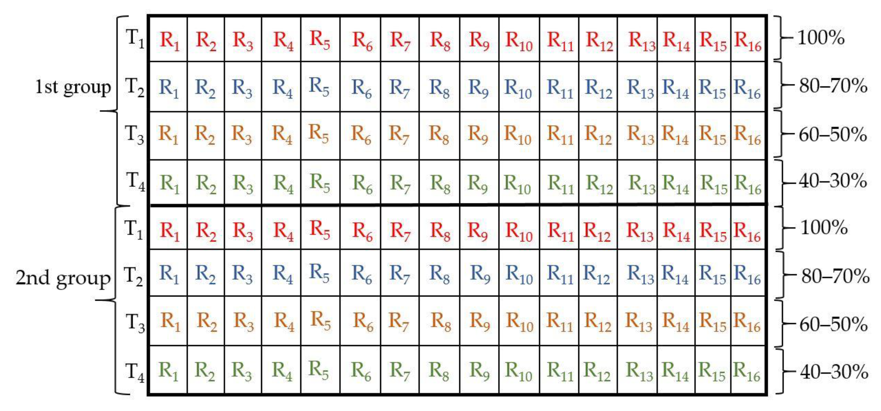
In an outdoor experiment, 128 potted plants of rice were grown under natural conditions at Zhejiang University (120°09′ E, 30°14′ N), Hangzhou City, Zhejiang Province, P.R. China. Frequently, a plastic cover was installed over the plants during precipitation to control the added water of plants, and obtain a heterogeneous water status of the tested leaves. To prepare experiment samples, the rice seeds (Xiushui 134) were submerged in the water for four days at a temperature of 28–30 °C, and the water was replaced twice a day. After germination, the 10 rice plants were sown into individual polyvinyl chloride (PVC) pots, which had dimensions of 140 × 95 × 125 mm. Each pot was filled with 300 g of black peat moss (HAWITA Gruppe GmbH, Vechta, Germany), and was irrigated to achieve saturation during the first growing month. The compound fertilizer treatment was applied, N–P2O5–K2O (15–15–15), with a rate of 100 kg ha−1 at 10-day intervals produced by Qingdao SONEF Chemical Company (Weifang, China). Potted rice plants were transplanted on 10 July 2018 and divided into two groups, each with 64 pots. It was harvested on 12 August and 30 August 2018 for the 1st and 2nd groups, respectively. Table 1 shows summary statistics of air temperature, relative humidity and vapor pressure deficit (VPD). The values of VPD were determined from the formula stated by [47]. In this experiment, there were two different growth stages of the rice plants: tillering and stem elongation. The water deficit was implemented within a time period of 27–34 days and 34–52 days of plant life for the 1st and 2nd groups, respectively. As displayed in Figure 1, an experiment was conducted with a completely randomized block design in a factorial experiment. The experimental design was divided into two groups, each comprising four irrigation treatments; fully-irrigated (T1: 100%), mild (T2: 80–70%), moderate (T3: 60–50%), and severe water stress (T4: 40–30% field capacity), respectively. The number of treatment replicates (R1, R2, …, etc.) was 16 samples. Generally, the gravimetric method was used to calculate the amount of water by weighing pots manually twice a day, followed by replacing the water transpiration to keep the respective moisture stress conditions. Gross water applied volumes were estimated for each group, 1st group values were 70.96, 66.64, 63.04, and 59.44 L (liter) for well-controlled, mild, moderate, and severe stress conditions, respectively. In addition, their corresponding values at the 2nd group were 96.56, 90.16, 85.36, and 78.96 L, respectively.

Table 1.
Brief measurements of climate factors.
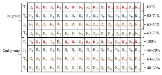
Figure 1.
An experimental design layout.
2.2. Hyperspectral Images Acquisition
The rice plants were moved from the outdoor environment to the laboratory. The spectral images were acquired by the near-infrared hyperspectral imaging system (874 to 1734 nm with 256 bands at each image). The system was integrated into a darkroom, which included an imaging spectrograph (ImSpector N17E; Spectral Imaging Ltd., Oulu, Finland), a 326 × 256 pixels camera (Xeva 992; Xenics Infrared Solutions, Leuven, Belgium), a camera lens (OLES22; Specim, Spectral Imaging Ltd., Oulu, Finland), two 150 W tungsten halogen lamps (3900 Lightsource, Illumination Technologies Inc., Elbridge, NY, USA) located on two sides of the camera at 45° angle, and a conveyer belt driven by a stepping motor (Isuzu Optics Corp., Taiwan, China). This system was fixed using one platform and controlled by a computer with preprocessing software (Spectral Image-VI0E, Isuzu Optics Corp., Taiwan, China). The camera focus was set to get high-quality images. The exposure time of 8 ms, the height between the samples and the lens, and the conveyor belt’s moving speed were 200 mm, and 30 mm/s, respectively. The imaging system in this study has previously been used for predicting the internal quality of kiwifruits [48]. The hyperspectral images were calibrated to decrease noise and avoid the influence of dark current [49] using the following formula:
where Idark is the dark reference image, Iwhite is the white reference image with 99.9% reflectance, Ic is the modified image, and Iraw is the raw image.
2.3. Image Preprocessing
The hyperspectral images preprocessing are necessary before data analysis to remove defects that may be introduced during the imaging period or in the image processing steps and facilities model training. It consists of such steps as image segmentation to remove background, noise reduction to remove outliers, and transformation to re-scale the features (normalization). Firstly, the region of green leaves in a pot was segmented as the region of interest (ROI). This procedure was performed by the ROI tool in ENVI 4.6 software (ITT, Visual Information Solutions, Boulder, CO, USA). The mean spectra of the ROI were calculated for further analysis. The range of ROI size was from 18,500 to 19,200 pixels for all collected images. Secondly, the signal-to-noise ratio (SNR) was estimated from the mean and standard deviation of sequential images, for each wavelength band, at each pixel. The allowable values of SNR are between 0.5 and 2.0 [50]. In this work, the bands with SNR lower than 2.0 were removed, such as the spectral range of 875–935 nm and 1670–1734 nm. So, the spectral range of 935–1670 nm with a total of 219 bands was considered for further analysis. Thirdly, normalization is transformed across individual features (f) to adjust for differences in magnitude between different features. Feature normalization (fnorm) is computed by subtracting the minimum image data (fmin) and by dividing the difference between the maximum (fmax) and the minimum feature value as shown by the following formula:
2.4. Canopy Water Content Computation
To provide a reference for data analysis, we collected the leaves of the ROI after taking the hyperspectral images, and the CWC of rice was measured. These leaves were weighed before drying. Then, the dry weight was obtained after drying the sample for 24 h in an oven at a temperature of 70 °C. The percentage of canopy water content was estimated by this formula:
where FW and DW are the fresh and dry weight of the canopy, respectively.
CWC (%) = (FW − DW)/FW × 100
2.5. Dataset and Data Analysis Software
A total of 128 images were split into training, validation, and testing, where 70% (89 samples) was used for the training and validation process of the regression model, while the other 30% (39 samples) was used to verify the model’s performance by comparing the expected CWC values with the calculated CWC values. A leave-one-out cross-validation (LOOCV) approach was utilized to train and validate the model. LOOCV excludes one sample for validation and uses the rest of the samples for training in every trial. This method can decrease over-fitting and permit a more accurate assessment of model prediction strength [51,52]. The feature selection, model establishment, and data analysis were implemented using Python 3.7.3. The PLSR, RF, and BPNN modules from the Scikit-learn library version 0.20.2 were used for regression tasks. The software was run on a PC with Intel Core i7-3630QM, 2.4 GHz CPU, and 8 GB RAM.
2.6. Overview of the Proposed Methods
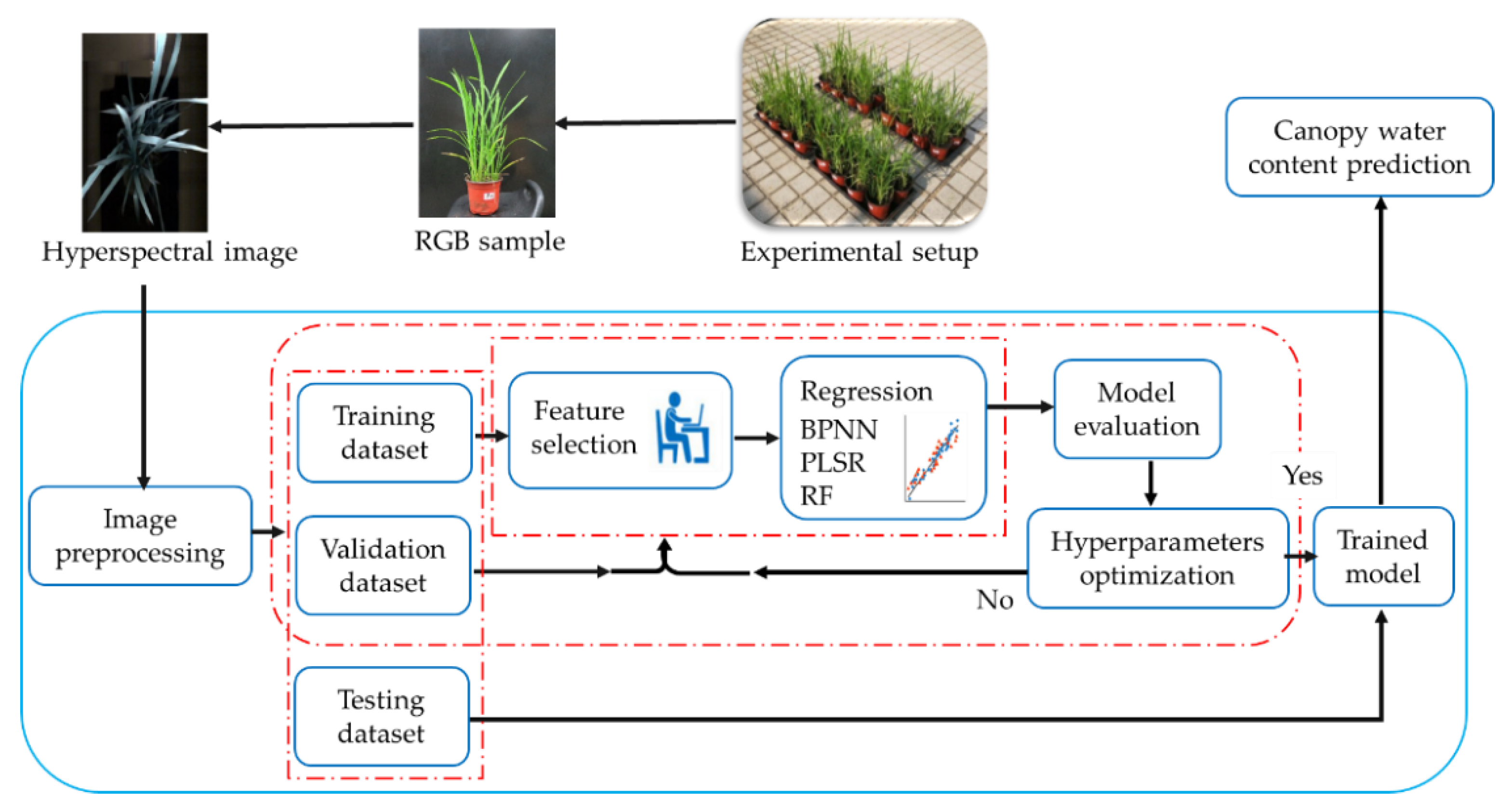
In this work, we proposed to combine some feature selection methods (VI, MF, and PCA) with machine learning regressors for the optimization of the prediction of water status in rice crops. Specifically, the proposed framework includes sequential steps as described in Figure 2: (a) spectra extraction from hyperspectral images; (b) split the dataset and train different algorithms using proposed features that served as inputs to the models; (c) select the best features, then check the model’s performance; (d) update hyperparameters in all models to achieve minimum root mean squared error of cross-validation (RMSECV); (e) if the model shows better performance, so we save the model; and (f) check the robustness of the model on new samples.
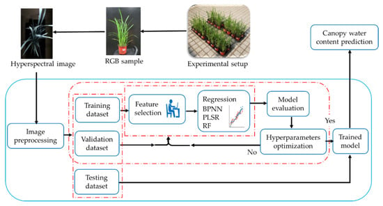
Figure 2.
Flow-chart of the methodology used for the present study.
2.7. The Spectral Features
2.7.1. Vegetation Indices
There are several spectral vegetation indices (VI) that are sensitive to the water condition of the plant; selecting the most appropriate VI needs to be tested [53]. So, this study involved examining the spectral VI potentials for estimating CWC of rice plants. According to previous studies, we utilized various VI, which are related with CWC including SB, WBI, NDVI, TBR, and SRI as shown in Table 2. Three indices were also adopted as new indices for this study that are discussed in the results section.

Table 2.
Spectral reflection indices used to assess water content in the canopy in this study.
2.7.2. Spectral Bands
The best spectral bands were designated by training three algorithms; PLSR, RF, and BPNN. After optimizing hyper-parameters, all bands were arranged and the optimal wavelengths were selected based on statistics of variables significance in the BPNN and RF model or the coefficients of each feature in the PLSR model. There are more details on picking the optimal wavebands in Section 2.8.
2.7.3. Feature Extracted from PCA
One hyperspectral image includes 219 bands and each band matches a gray image. The textural characteristics set are enormous and hard to measure. The PCA strategy is a suitable tool for decreasing the number of dimensions in the data to only use the wavelengths that contribute most to machine learning regression tasks. It contains several principal components (PC) that have sufficient valid data instead of all spectra with the whole dataset [58]. The first PC describes the biggest variance and subsequently reduces the variables described in the following components. However, the inclusion of too many latent variables led to over-fitting [37]. In this work, we estimated about six bands that were the most contributing to the first two PC. Then, these wavebands were used as inputs for the proposed models to check the performance of each model and select the best one.
2.8. Training Models Based on MF and Feature Selection
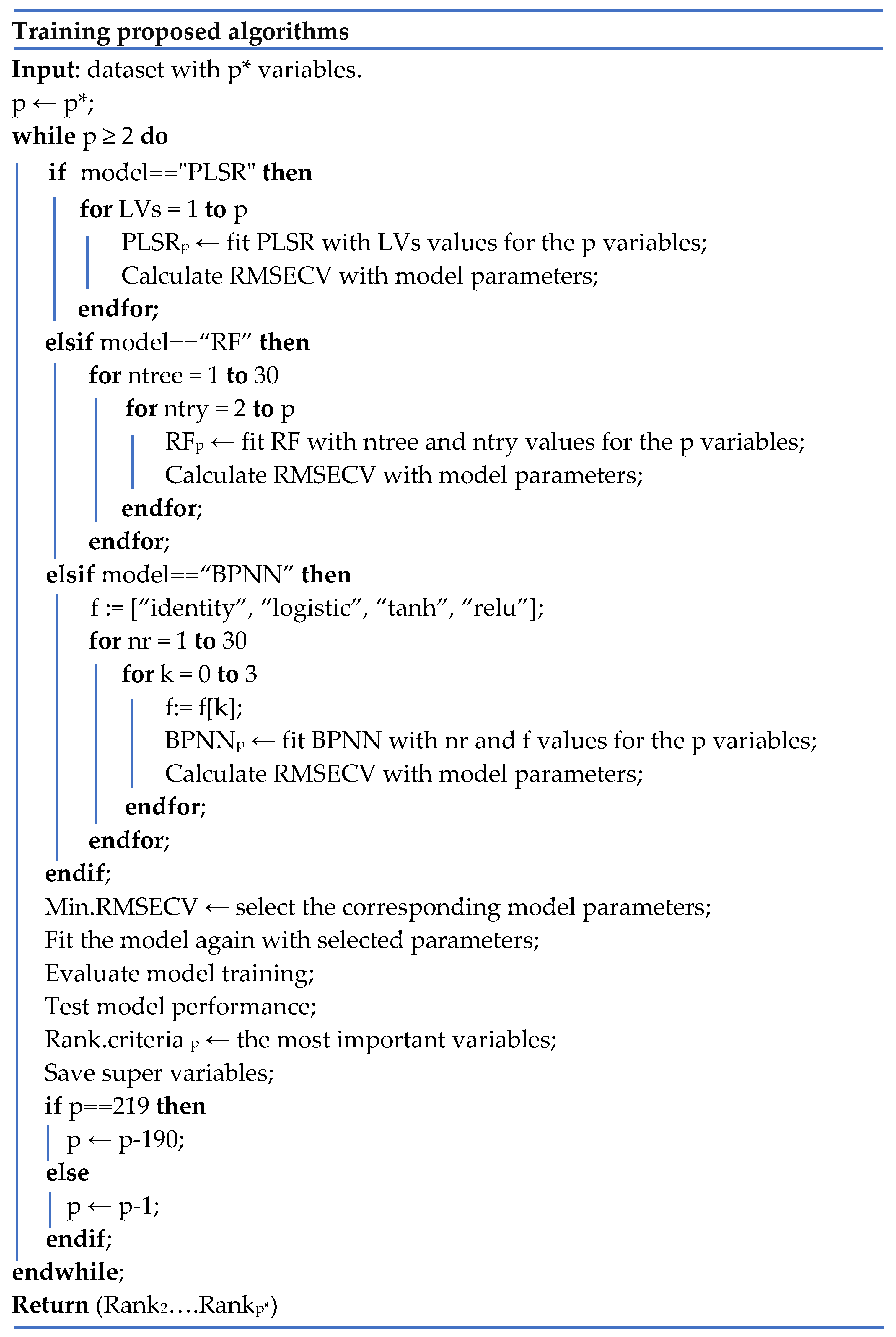
One of the purposes in this research was to compare different features with regression models. The three types of the dataset (samples × features) for analysis were (89 × 12), (89 × 219), and (89 × 6). These data were employed for training three regression models; PLSR, RF, and BPNN. We optimized the models by selecting the best hyperparameters. The parameters were an optimal number of latent variables (LVs) with PLSR, the number of trees (ntree) and features (ntry) at every tree node for training RF model, number of neurons in the hidden layer (nr), and activation function (f) in the BPNN model. The main steps for training the models, and estimating the right parameters and features are described in Figure 3. This figure illustrates the pseudo-code for each model in order to achieve a combination of optimal features of at least 2 variables. The number of features in each loop was at spectral bands; 256, 29, 28, …, 2, vegetation indices; 12, 11, 10, …, 2, and PCA bands; 6, 5, 4, …, 2. During looping, the most important features were picked up and the rest were excluded. Then, it was easy to compare all outputs to determine the best features set that could improve the prediction of water content in rice.

Figure 3.
Pseudo-code to train each algorithm and select the top variables.
2.8.1. Partial Least Square Regression (PLSR)
The parameter of LVs was determined according to the lowest value of the root mean squared error of cross-validation (RMSECV) using the leave-one-out validation method (LOOV). We followed the same procedure proposed by the Backward Variable Selection method for PLS regression (BVSPLS) to identify the optimal features [59]. After calculating LVs, the model was refitted again to get the final model. Then, the features were sorted out ascendingly based on the coefficients for the studied features in the PLSR model. At each iteration, the number of features was gradually reduced. The best LVs value and the highest features were chosen based on the lowest RMSECV.
2.8.2. Random Forest (RF)
It is a bagging method based on the classification and regression tree (CART). It uses recursive partitioning to split the data into many homogenous subsets known as regression trees (ntree) and then averages the results of all trees. Each tree is separately grown to its maximum size based on a bootstrap sample from the training data set without stopping the picking of the input variables at each node. In each tree, RF uses randomness in the regression process by selecting a random subset of variables (mtry) to determine the split at each node [60]. In this model, the two parameters (mtry and ntree) were optimized with less RMSECV using the LOOV method. The ntree value was tested in the range from 1 to 30, and the mtry value was evaluated by a different number of features. After training the model with optimal parameters, all features were arranged and the finest features were selected based on variable importance statistics [33]. The outputs were collected during all iterations and different alternatives for the best features combination were examined to select the best one that achieved the lowest RMSECV.
2.8.3. Back-Propagation Neural Network (BPNN)
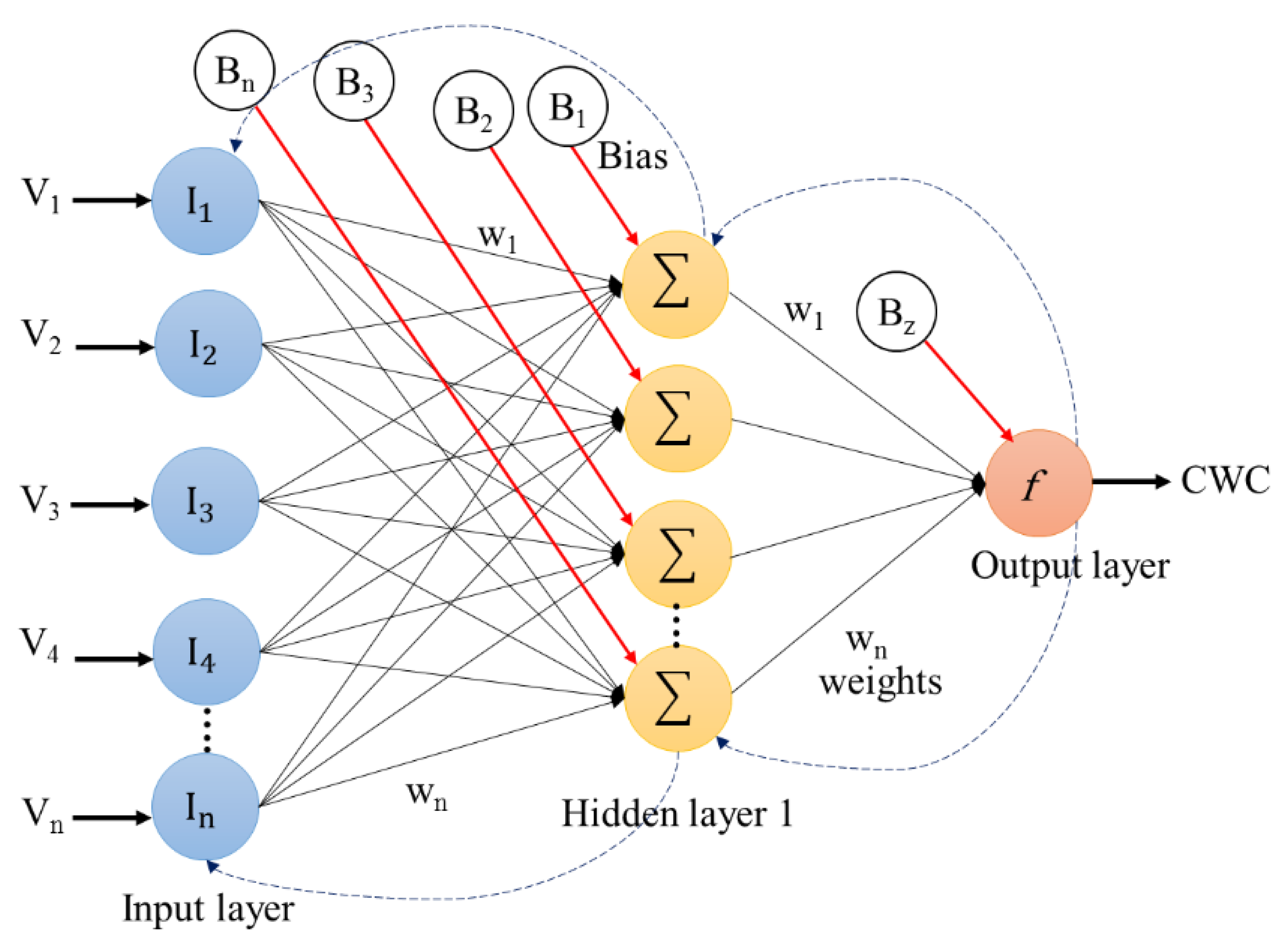
This network uses the Multi-Layer Perceptrons (MLPs) as a supervised learning algorithm that includes a flexible function to train a specific data set [61]. MLPs is one of the neural network models, has the same architecture of back-propagation for supervised training. Back-propagation is typically used for training of feed forward. The neural net is structured from three types of layers: (1) the input layer is primary data for the neural network; (2) the hidden layer is an intermediate layer between independent inputs layer and dependent output layer, and (3) the output layer produces the results of the specified inputs. Figure 4 displays the architecture of the neural artificial network is a class of machine learning algorithms that uses multiple layers to gradually extract high-level features from the raw input. Five circles as input layers are noted as vector I. The network contains one hidden layer, the number of nodes determined according to regression accuracy. Four circles with one hidden layer represent the “activation” nodes and are usually noted as weight (W). The final circle refers to the output layer that shows the predicted value of canopy water content. The bias neuron (B) is a special neuron added to each layer in the neural network, which is usually taken to be 1 [62]. The artificial neural network models are generalized mathematical models that use a series of neurons or nodes interlinked by weighted connections to simulate human cognition as it applies to pattern identification and prediction [63,64].
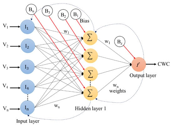
Figure 4.
Architecture of neural artificial network.
In this research, the input variables involve 12 VI, 219 spectral bands, and 6 PCA bands. A mathematical model is given in the following equation, where y is the output value, I1, I2, …, In signifies the nth input variables, W1, W2, …, Wn indicates the nth weights of the combination which produces the output, θ is the unit step function, W is the weight-related with the Ith input and μ is the average.
The generalized weight W is realized as the contribution of the Ith covariate to the log-odds, and the equation below defines the generalized weight:
The network was trained for at least 1000 iterations or until the error measurement approached (). To choose the number of neurons in the hidden layer for this model, the cross-validation technique with the LOOV method was performed on the training dataset. The parameter of limited memory Broyden–Fletcher–Goldfarb–Shanno (lbfgs) was used as a weight optimizer to implement the algorithm efficiently [65]. To improve the predictive capacity of the regression model and reduce hyperspectral image dimensionality, the following formula was used to determine the most informative features [34]:
where M is the important measure for the input variable, is the number of input variables, is the number of hidden layer nodes, is the absolute value of the hidden layer weight corresponding to the pth input variable and the jth hidden layer, and is the absolute value of the output layer weight corresponding to the jth hidden layer.
2.9. Model Evaluation
To measure the performance of a regression model, the following statistical indicators have been chosen: root mean square error (RMSE), mean absolute percentage error (MAPE), prediction accuracy (Acc), and coefficient of determination (R2) [66,67]. All parameters are explicated as follows: CWCact is the actual value that was estimated from laboratory calculations, CWCp is the predicted or simulated value, CWCave is the average value, and N is the total number of data points.
3. Results and Discussion
3.1. Effects of Water Deficit Stress on Spectral Reflectance Pattern
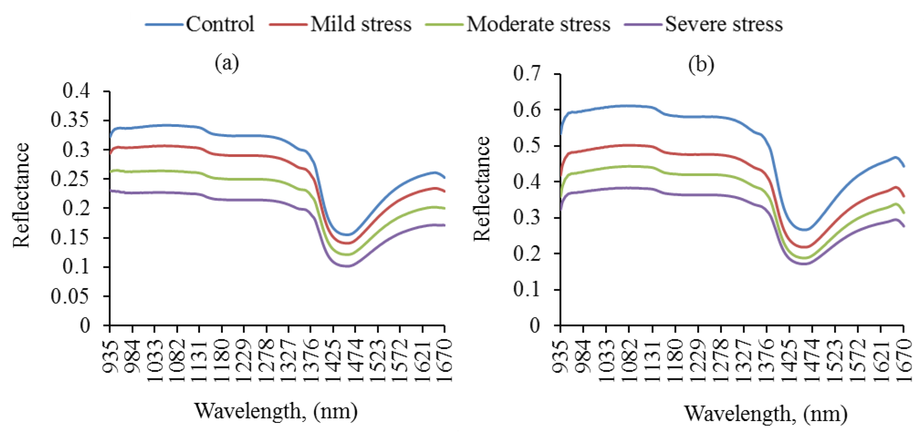
The average reflectance spectra under different water stress conditions during two growth stages of rice plants are explained as shown in Figure 5. The values of mean soil water content in the 1st stage (tillering) were 88, 78, 66, and 49% for well-controlled, mild, moderate, and severe stress conditions, respectively. Moreover, their corresponding values in the 2nd stage (stem elongation) were 85, 72, 60, and 40%, respectively. At the band of 1450 nm, the figure shows that the height of the valley decreases as water content decreases where there is strong water absorption. A greater increase in canopy reflectance was observed in the NIR region for the control treatment and low reflectances for soil moisture stress treatments. Besides, the rice water content in the 2nd stage is greater than the 1st stage, and the spectrum at the 2nd stage was showing a higher reflection trend. These results are in agreement with Carter [68,69] who explained that the absorption by pigments and water in the range of near-infrared (NIR; 700–1300 nm) is relatively low, thus, the reflectance is relatively high. In addition to [70], higher absorption of infrared radiation resulted in leaf heating and transpiration. Hence, the lower reflectance in the NIR region further confirmed the soil moisture stress-induced reduction in transpiration and stomatal conductance in the rice canopy at its vegetative stage. The pattern of the reflectance curves is close to that for other green plant leaves such as maize [71].
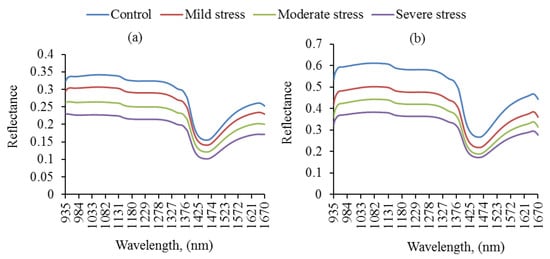
Figure 5.
Average spectral reflectance after removing outliers for rice samples under different levels of water deficit at two growth stages: (a) tillering and (b) stem elongation.
3.2. The Features
3.2.1. Vegetation Indices (VI)
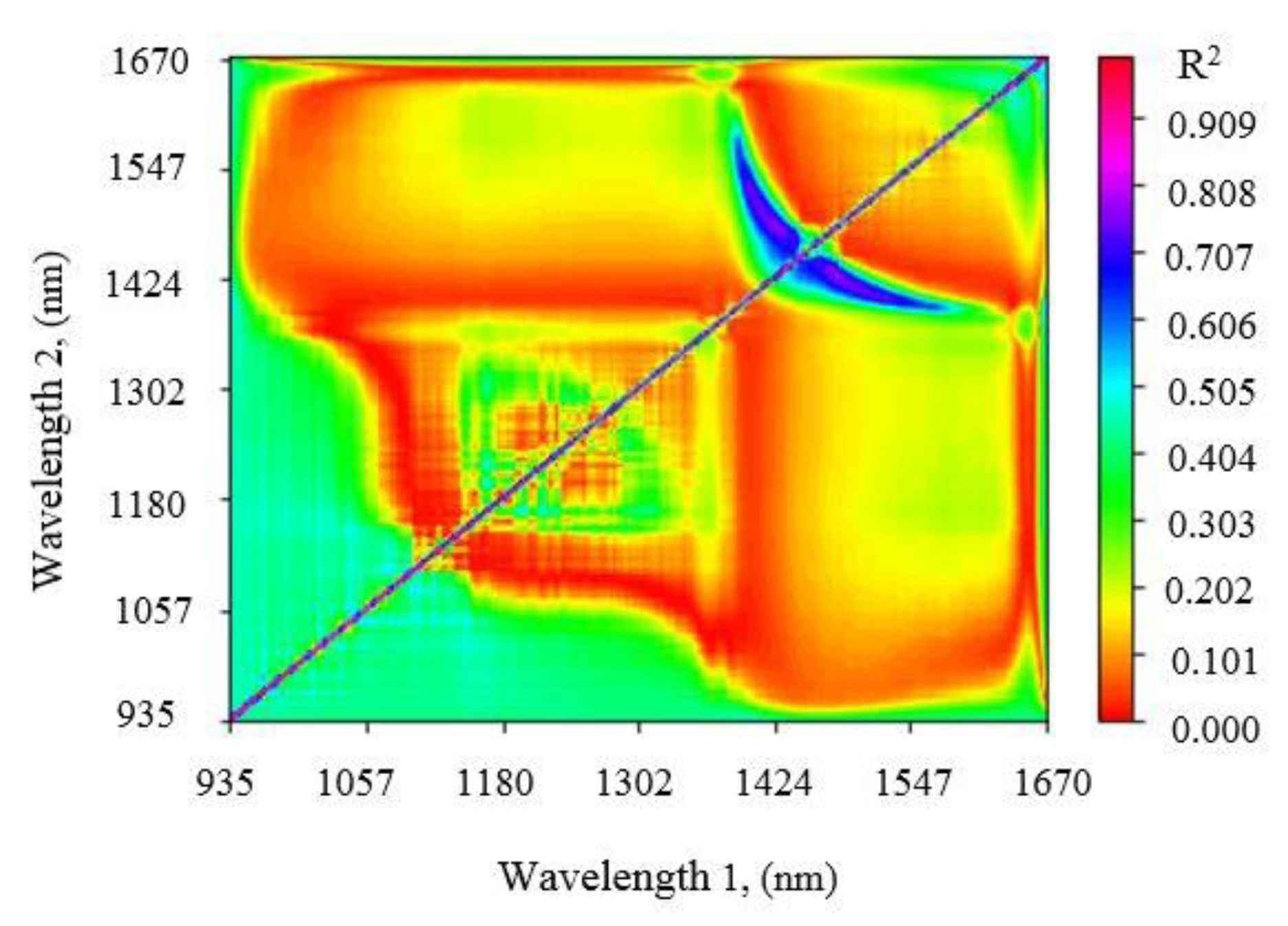
The contour map as shown in Figure 6 presents more reliable and strong relationships with rice water content based on the coefficient of determination (R2) for all dual wavelength combinations. The contour plotting using the simple ratio index (SRI) was done in all possible combinations within 935–1670 nm and their correlations with CWC were quantified to identify the best index. We adopted about 3 indices as a case study; SRI#1 (R1426/R1480), SRI#2 (R1480/R1429), and SRI#3 (R1433/R1477), which their values at R2 were 0.777, 0.762, and 0.759, respectively. The new spectral indices formula in this study was R1/R2 through water stress treatments. The R2 values between the suggested spectral indices in this analysis and the CWC for rice were 0.945 (SB-1), 0.969 (SB-2), 0.442 (WBI-1), 0.265 (WBI-2), 0.012 (NDVI-1), 0.462 (NDVI-2), 0.039 (TBR), 0.463 (SRI-1), and 0.027 (SRI-2), respectively. The best prediction indices were chosen after training different models according to the model performance.

Figure 6.
Determination coefficients for all dual wavelength combinations of hyperspectral reflectance.
3.2.2. Model-Based Features (MF)
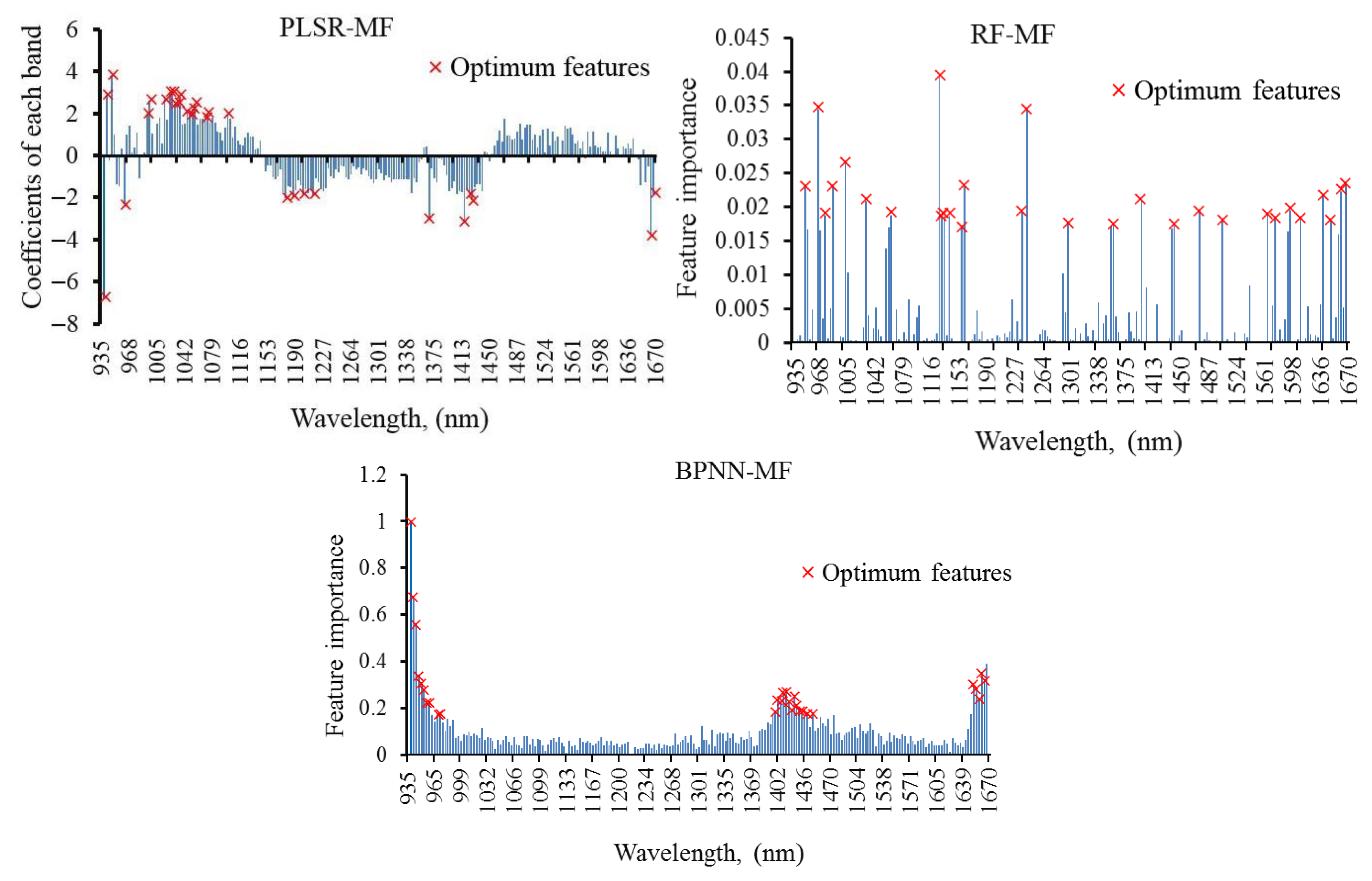
This technique was employed with spectral wavelengths to choose the optimal bands after training the models. Three regression models (PLSR, RF, and BPNN) were optimized with the best parameters. During the 1st loop, the number of variables needed for water content prediction in rice was substantially reduced from 219 to 29 bands. The selection of the most important bands varies with the different regression models as exhibited in Figure 7. Optimized models were established using these wavelengths as displayed in Table 3. At PLSR-MF model, the ideal number of LVs with the lowest value of RMSECV (0.914) was estimated by six factors. The prediction ability of this model with the selected wavelengths increased equivalent to the model with full spectra, with prediction R2 (0.928 vs. 0.918), and RMSECV (0.867 vs. 0.914). At RF-MF model, the ntree and mtry for expecting CWC were recorded with 40 trees and 38 features, respectively. This model was improved with prediction R2 (0.997 vs. 0.996) and RMSECV (0.193 vs. 0.212). At BPNN-MF model, the excellent performance was verified for estimating the water content by 28 neurons in a single hidden layer and logistic as an activation function. The prediction R2 increased from 0.879 to 0.996 and RMSECV decreased from 0.329 to 0.286.
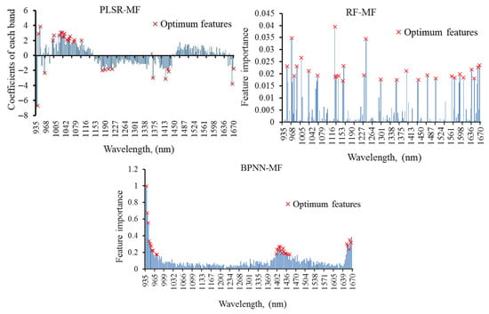
Figure 7.
Selection of most contribution features using partial least square regression (PLSR), random forest (RF), and back-propagation neural network (BPNN) models during the first loop.

Table 3.
Ranking of features in order of importance for different regression models during the 1st loop.
3.2.3. The Best Bands Extracted from PCA
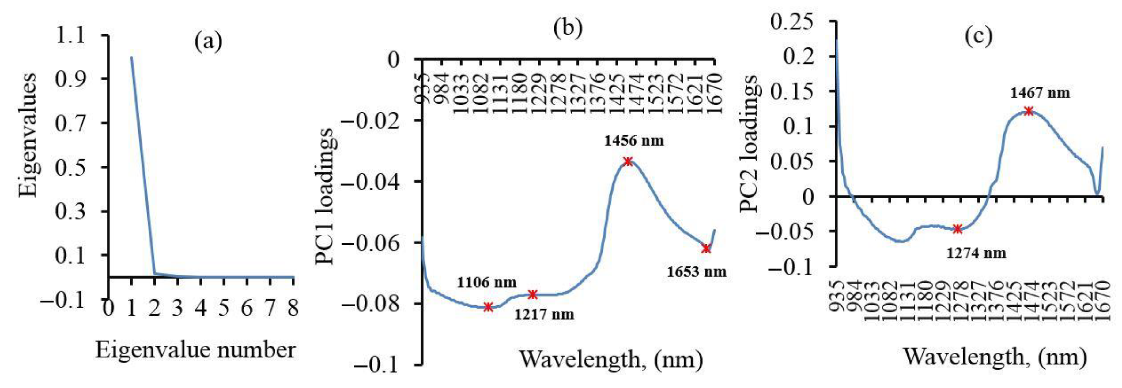
The optimal bands were selected in which 99.87% of the variance was described by the first two of PC and accounted for 98.37% and 1.5% of the total spectral variation at PC1 and PC2, respectively. The loadings caused by PCA were explained as an indication of effective wavelengths, which were responsible for the specific characteristics of the respective scores, contributing to the prediction of CWC. In those specific principal components, the wavelengths corresponding to the tops and valleys were chosen to be ideal wavelengths as displayed in Figure 8. The most significant wavebands were 1106, 1217, 1456, 1653, 1274, and 1467 nm. The PCA analysis was based on eigenvectors with the highest sensitivity to water content and later, it can be used to identify CWC in rice instead of the entire spectrum. These results are close to previous reports; the reflectance at 1450 nm is sensitive to water status in leaf [68]. In addition, the wavelengths related to a range of 1500–1750 nm have been known to be necessary to observe the water status of the plant [72]. Besides, the 1200 nm wavelength represents an absorption feature and indicates a robust prediction for CWC and the leaves [73].
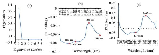
Figure 8.
(a) The proportion of variance of reflectance data described by the two eigenvectors with the largest eigenvalues, and wavelengths selection from loadings of the first two principal components: (b) PC1-loadings, and (c) PC2-loadings.
3.3. Assessment of Regression Models
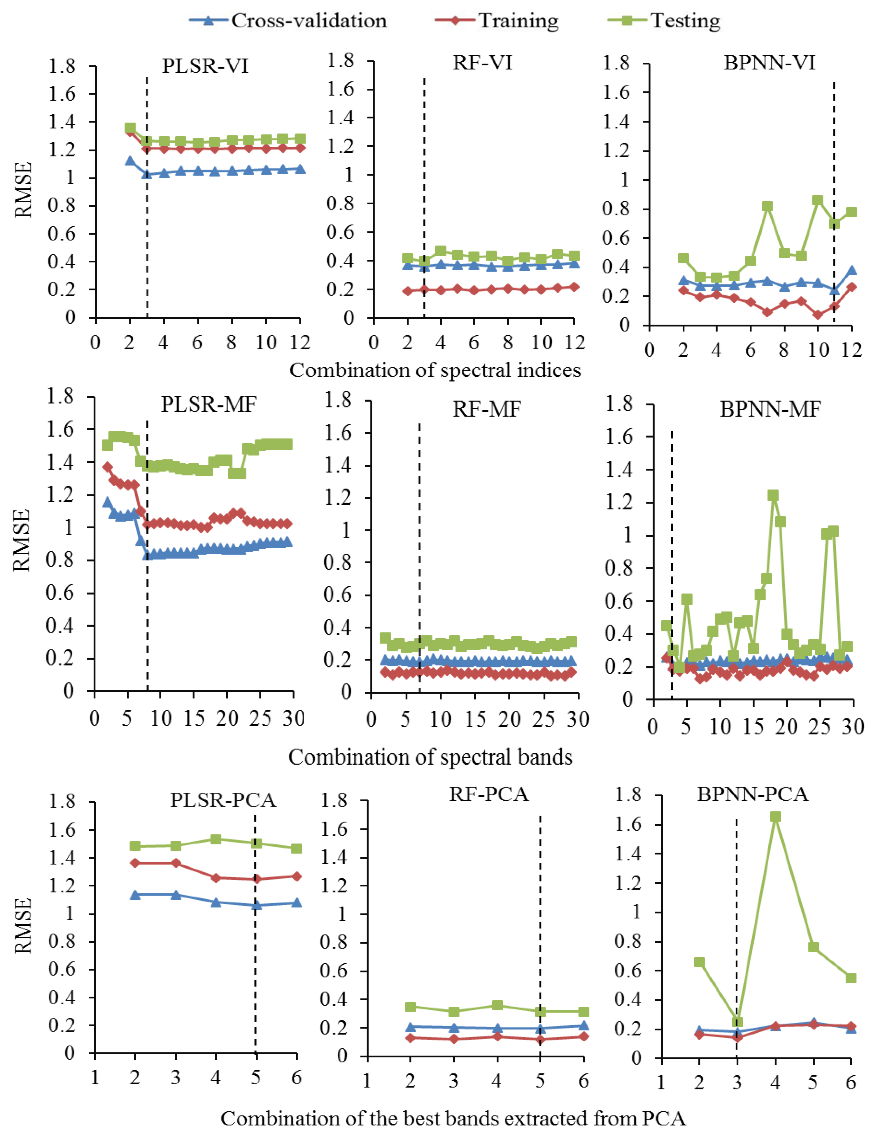
There are three types of features for predicting the water content in rice: (1) the best bands selected from PCA; (2) picking the optimum bands after training variables, that is model-based features (MF), and (3) vegetation indices (VI). These features were trained with different models (PLSR, RF, and BPNN) and the less important features were excluded. Al Iqbal [74] explained that some features are less important, however, some are very significant. The superlative model and the ideal combination of features were chosen when a minimum RMSECV value was reached.
From the results, the model prediction accuracy depends on the value and number of features. Various options for combining features and models were collected as shown in Figure 9. This figure explicates that there are specific features of training the models that have the lowest RMSECV value and are excellent in forecasting. These features are presented in Table 4, which are the highest contributing variables for the CWC prediction in rice. The RMSECV value decreased with these selected features depending on the model applied. The lowest and largest RMSECV values were 0.183 and 1.063, which were obtained with the superb model of BPNN-PCA-MF-3 and the less accurate prediction model of PLSR-PCA-MF-5, respectively.
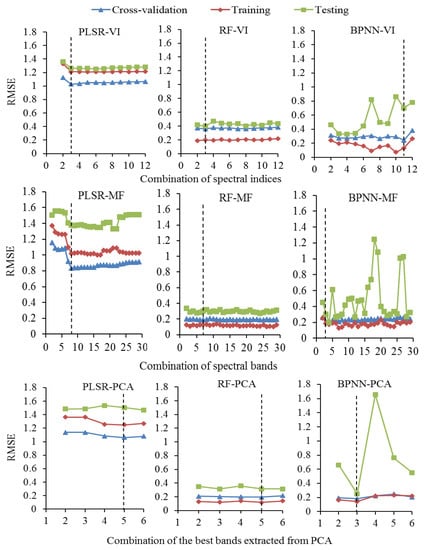
Figure 9.
Comparison of various combinations of regression models and feature selection methods based on best features and lowest root mean squared error of cross-validation (RMSECV).

Table 4.
The best selected features with different regression models after completing all loops.
The performance of the generated models was compared based on full and optimal features as shown in Table 5. This table illustrates the number of proposed features, best parameters, Acc and model outputs for RMSE, MAPE, and R2 via training, cross-validation, and test set. Outcomes of advanced models after adopting the best features were optimized. The ranking of high-performance models based on the lowest RMSECV is as follows: Firstly, the VI-based models were BPNN-VI-MF-11, RF-VI-MF-3, and PLSR-VI-MF-3, respectively. The BPNN-VI-MF-11 model was superior in the prediction of CWC and was built with 10 hidden neurons and logistic function. This model enhanced R2, RMSE, MAPE, and Acc to 0.981, 0.736, 0.610%, and 0.994, respectively. The PLSR-VI-MF-3 model achieved a high expectation at LVs of 3. The performance rose to 0.943, 1.265, and 1.349% for R2, RMSE, and MAPE, respectively. The value of Acc was 0.986. Secondly, the MF-based models were RF-MF-7, BPNN-MF-3, and PLSR-MF-8, respectively. The RF-MF-7 model was established through 20 ntree and 3 ntry. The R2 increased to 0.997, while RMSE and MAPE decreased to 0.299 and 0.259%, respectively. The score of Acc was 0.997. At PLSR-MF-8 model, the cross-validation at LVs of 5 was optimized by 8 bands. Model behavior improved with R2 (0.932), RMSE (1.376), MAPE (1.440%), and Acc (0.986), respectively. Thirdly, the PCA-based models were BPNN-PCA-MF-3, RF-PCA-MF-5, and PLSR-PCA-MF-5, respectively. The BPNN-PCA-MF-3 model contained the top variables for predicting the water content of rice and was constructed using 28 hidden neurons and logistic function. The performance of this model with R2, RMSE, MAPE, and Acc was 0.998, 0.252, 0.259%, and 0.998, respectively. The PLSR-PCA-MF-5 model was created with LVs of 5. Its outputs with R2, RMSE, MAPE, and Acc were 0.919, 1.504, 1.634%, and 0.983%, respectively.

Table 5.
Evaluation of different regression models with all proposed features and best-specified features.
The results suggested that robust prediction accuracy for CWC could be achieved if suitable algorithm and higher variables were assigned. This was similar to Krishna et al. [75], who exhibited a comparison of various regression models for relative water content monitoring in rice based on spectral data. They selected the best bands by the PLSR model. The prediction model performance was arranged based on R2 and RMSE as follows: PLSR-MLR > PLSR-BPNN > SVR > RF > PLSR > BPNN; where MLR and SVR are multiple linear regression and support vector machine regression models, respectively. The performance of the PLSR-MLR model was (R2 = 0.98 and RMSE = 3.19 for calibration and R2 = 0.97 and RMSE = 5.06 in validation). Compared to previous research, an advanced model of PBNN-PCA-MF-3 in this work performed more accurately than the PLSR-MLR model. Moreover, the outputs of the developed models are very precise compared to Sun et al. [71] who indicated that an acceptable model for estimating CWC in wheat based on Ratio Vegetation Index (RVI; 1605 and 1712 nm) and Normalized Difference Vegetation Index (NDVI; 1712 and 1605 nm) having the highest R2 and lowest RMSE in model calibration and validation (R2c = 0.74 and 0.73; RMSEC = 0.026 and 0.027; R2v = 0.72 and 0.71; RMSEV = 0.028 and 0.029). Furthermore, these results were better than Ge et al. [76] who concluded leaf water content in maize at a pot-scale is successfully predicted with the hyperspectral images using the PLSR model for two genotypes in model cross-validation (R2 = 0.81 and 0.92; RMSE = 3.7 and 2.3; MAPE = 3.6 and 2.2). Besides, the proposed models achieved high performance compared with Pandey et al. [77] who showed that PLSR analysis can be modeled to predict leaf water content for potted corn and soybean plants with the highest accuracy (R2 = 0.93, RMSE = 1.62, and MAPE = 1.6%) in the validation set.
3.4. Neural Network Topology with Higher Variants
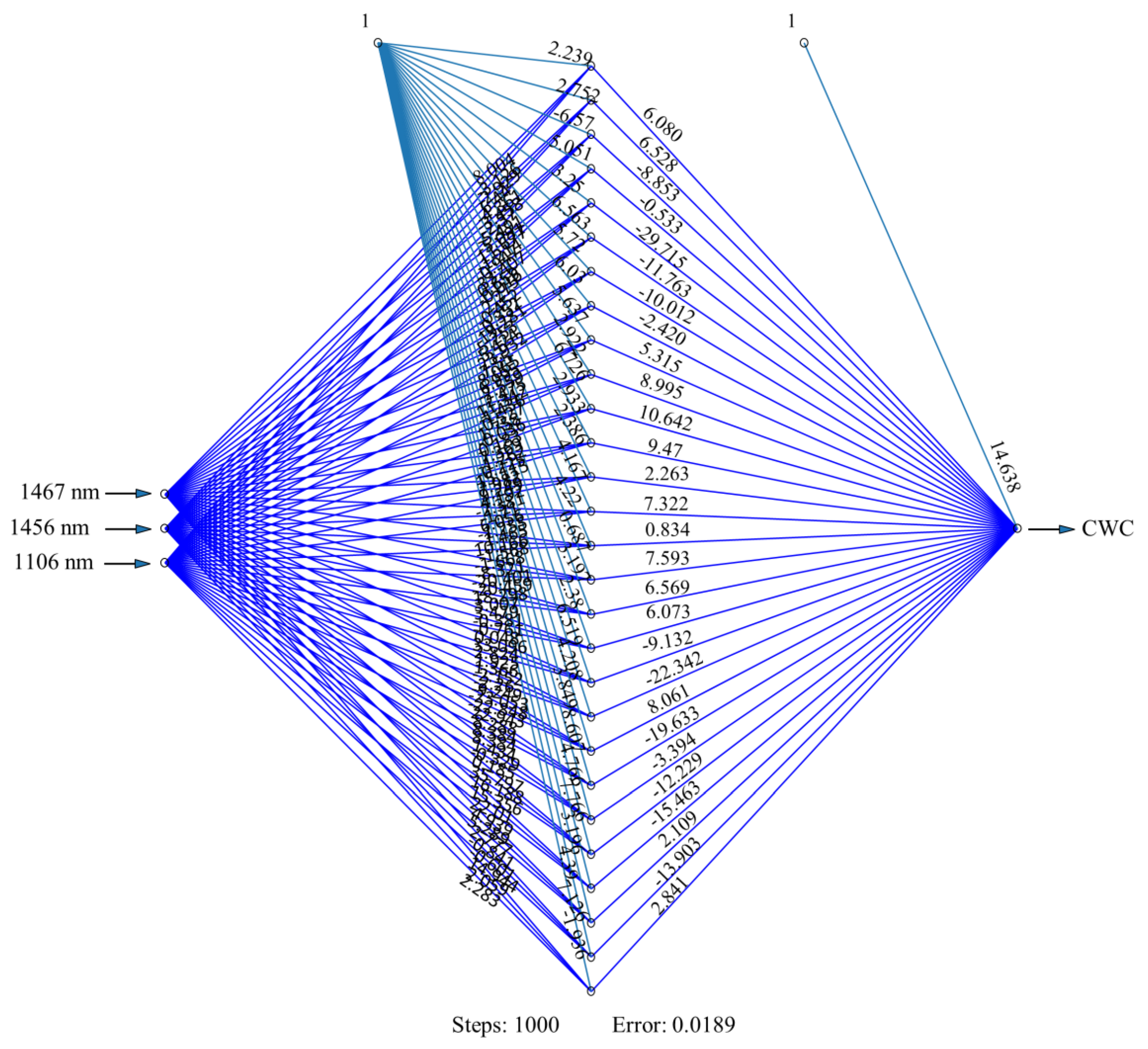
The neural network design after gathering senior features is presented in Figure 10. This figure showed the best structure of the trained neural network with the variants chosen. Neural network conveys basic information such as the trained synaptic weights, a number of hidden neuron layers, steps for converging, and the overall errors. Network topology is constructed with a specific combination of input variables with a number of hidden neuron layers. For example, an eminent model of BPNN-PCA-MF contains an input layer of 3 bands (1467, 1456, and 1106 nm) and a single hidden layer with 28 neurons as shown in Figure 10. The presented planning depicts the neural network with prominent bands; the training process needed 1000 steps to achieve less error function. The process has an overall error of about 0.0189. Furthermore, before nominating the most influential bands, the training process at 6 PCA bands needed 1000 steps with the process having an overall error of about 0.0251.
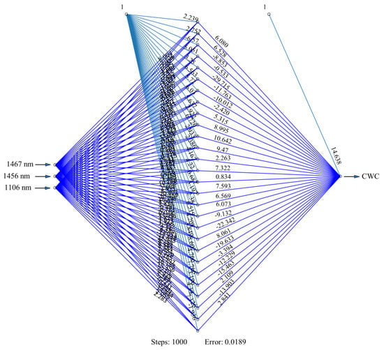
Figure 10.
Neural network topology for best-combined variants in the BPNN- principal component analysis (PCA)- model-based features (MF) model.
3.5. Canopy Water Content Prediction and Validation
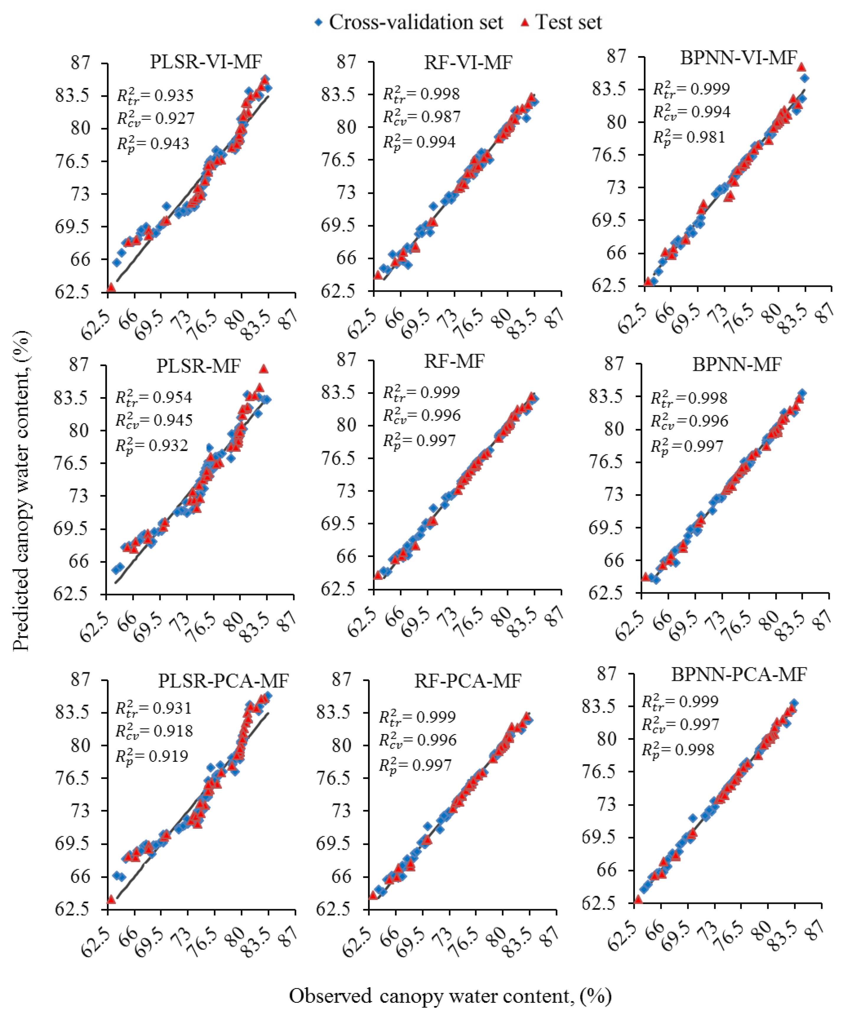
From the findings, the best feature selection method for estimating the canopy water content in rice was PCA combined with MF (PCA-MF). This was the premium integration to filter out the super variables. Moreover, the MF approach was combined with VI (VI-MF) to improve model performance. There are nine approaches as a new prediction methodology, including the integration of PCA-MF, VI-MF, and MF with three models: PLSR, RF, and BPNN. The regression models were trained with the uppermost features (independent variables) for predicting the CWC (dependent variable). The projected CWC values were then compared to the reserved values that were not implemented for machine learning. Figure 11 illustrates the scatter plots of the observed and predicted CWC in rice through integrating the proposed feature selection methods and the different models. This study evaluated multivariate methods and compared the results clearly, so the use of multivariate methods greatly enhances predictability. As well, independent validation can be considered the most robust method for assessing the accuracy of a regression model, because validation data are not involved in the process of model development. The BPNN-PCA-MF-3 was the first best predictive model as evidenced by the performance and showed a stronger relationship between the reflectance spectra and CWC. The predictability of this model was developed by PCA that can select optimum wavebands and eliminate data redundancy and outliers [78], then select the most critical bands on the basis of the MF. The values of R2 at BPNN-PCA-MF-3 were 0.997 and 0.998 for cross-validation and test set, respectively. This model can reduce the regression error to a minimum (RMSE = 0.183 in cross-validation) for predicting the water status. The three bands involved in this model are of great importance in predicting water content. The RF-MF-7 model was the second-ranked according to performance. The RMSE value in cross-validation was 0.189. Its outputs with R2 were 0.996 and 0.997 for cross-validation and test set, respectively. The third most reliable model was RF-PCA-MF-5 with an RMSE of 0.197 in cross-validation. The R2 was 0.996 and 0.997 for cross-validation and test set, respectively. The results explained that the performance of PLSR with VI-MF, MF, and PCA-MF was a less predictive model (R2 = 0.943, 0.932, and 0.919 in prediction, respectively) compared to others to monitor the water condition in rice. This is agreed with Krishna et al. [79] who described that each coefficient in the PLSR model has an associated RMSE, making it more prone to deviation. As a result, the combined model of PLSR with different feature selection approaches was less-performing for predicting CWC.

Figure 11.
The correlation between predicted and observed canopy water content (CWC) using various combinations of best features in advanced models.
Otherwise, residual value plays a vital role to validate the obtained regression model. The difference between the actual CWC and the predicted CWC is the residual. We calculated the residual value with the first three higher models. At BPNN-PCA-MF-3 model, the residual was −0.637% and 0.492% for the lowest and highest residuals in predicted CWC, respectively. The lowest residual of −3.046% and highest of 0.526% were calculated with the BPNN-PCA-6 model. At RF-MF-7 model, the lowest and highest residuals were −1.023% and 0.753%, respectively, while the lowest residual of −1.053% and highest of 0.732% were calculated with the RF-MF-219 model. The lowest and highest residuals values were (−1.034% and 0.74%) and (−1.106% and 0.632%) with RF-PCA-MF-5 and RF-PCA-6 models, respectively.
Multivariate models have been applied with many studies to estimate different parameters in plant biochemical, i.e., chlorophyll [80], nitrogen [37], relative water content [22], and leaf equivalent water thickness [81]. These approaches use all relevant water absorption bands that greatly increase model performance by improving sensitivity to changes in the CWC. This work has been largely effective in increasing the model’s prediction efficiency through a finite number of an appropriate set of features. The generated models attained high correlation coefficients, high precision, and less deviation between the actual CWC and the predicted values. Finally, the results have provided basic guidance for water users and agricultural development planners for the optimal evaluation of the CWC that can assist in an appropriate assessment of crop water needs.
4. Conclusions
The present study explored the ability to apply hyperspectral imaging with machine learning algorithms to predict the canopy water content of rice. We evaluated some multivariate techniques including back-propagation neural network (BPNN), random forest (RF), and partial least square regression (PLSR) with different feature selection approaches such as vegetation indices (VI), model-based features (MF), and principal component analysis (PCA). The crop spectral reflectance was applied with different levels of water deficit to develop an algorithm that can predict the CWC. The regression algorithms have been upgraded for robust prediction of rice water status through some actions including high-level features nominating, hyper-parameters optimization, providing various alternatives for the most sensitive features, and integrating the model with the best-combined features. Then, the performance findings were compared to define a good-quality model. From experimental results, the supreme combinations for CWC prediction between regression models and feature selection methods according to the highest performance were BPNN-PCA-MF (R2 = 0.998 and RMSE = 0.252), RF-MF, (R2 = 0.997 and RMSE = 0.299), and BPNN-VI-MF (R2 = 0.981 and RMSE = 0.736), respectively. These developed models produced satisfactory outcomes with high accuracy and were adopted using 3, 7 bands, and 11 VI, respectively. The fusion of PCA-MF-based features with the BPNN algorithm achieved an excellent model for CWC prediction. At last, this tool is a rapid, convenient technique, and can assist water managers to make effective decisions in real-time. In the future, we recommend extending the use of the superlative model with other economic crops such as corn and wheat to achieve sustainable agricultural water management.
Author Contributions
O.E. performed the experiment, wrote all parts of the manuscript, and analyzed the data. Y.F. and L.Z. revised the manuscript. Z.Q. planned the overall study and supervised the research. All authors have read and agreed to the published version of the manuscript.
Funding
This work was supported by China National Key Research and Development Program (2016YFD0700304).
Data Availability Statement
The data presented in this study are available within the article.
Conflicts of Interest
The authors declare no conflict of interest.
References
- Gilbert, N. Water under pressure. Nature 2012, 483, 256–257. [Google Scholar] [CrossRef] [PubMed]
- El-Hendawy, S.; Al-Suhaibani, N.; Salem, A.; Ur Rehman, S.; Schmidhalter, U. Spectral reflectance indices as a rapid nondestructive phenotyping tool forestimating different morphophysiological traits of contrasting spring wheatgermplasms under arid conditions. Turk. J. Agric. For. 2015, 39, 572–587. [Google Scholar] [CrossRef]
- Peñuelas, J.; Filella, I.; Biel, C.; Serrano, L.; Save, R. The reflectance at the 950–970 nm region as an indicator of plant water status. Int. J. Remote Sens. 1993, 14, 1887–1905. [Google Scholar] [CrossRef]
- Peñuelas, J.; Piñol, J.; Ogaya, R.; Filella, I. Estimation of plant water concentration by the reflectance water index WI (R900/R970). Int. J. Remote Sens. 1997, 18, 2869–2875. [Google Scholar] [CrossRef]
- Clevers, J.G.P.W.; Kooistra, L.; Schaepman, M.E. Estimating canopy water content using hyperspectral remote sensing data. Int. J. Appl. Earth. Obs. 2010, 12, 119–125. [Google Scholar] [CrossRef]
- Penuelas, J.; Filella, I.; Serrano, L.; Save, R. Cell wall elasticity and water index (r970nm/r900nm) in wheat under different nitrogen availabilities. Int. J. Remote Sens. 1996, 17, 373–382. [Google Scholar] [CrossRef]
- Hank, T.B.; Berger, K.; Bach, H.; Clevers, J.G.P.W.; Gitelson, A.; Zarco-Tejada, P.; Mauser, W. Spaceborne imaging spectroscopy for sustainable agriculture: Contributions and challenges. Surv. Geophys. 2018, 40, 515–551. [Google Scholar] [CrossRef]
- Danson, F.M.; Steven, M.D.; Malthus, T.J.; Clark, J.A. High-spectral resolution data for determining leaf water content. Int. J Remote Sens. 1992, 13, 461–470. [Google Scholar] [CrossRef]
- Clevers, J.G.P.W.; Kooistra, L.; Schaepman, M.E. Using spectral information from the NIR water absorption features for the retrieval of canopy water content. Int. J. Appl. Earth Obs. 2008, 10, 388–397. [Google Scholar] [CrossRef]
- Scholander, P.F.; Hammel, H.; Bradstreet, E.D.; Hemmingsen, E. Sap pressure in vascular plants. Science 1965, 148, 339–346. [Google Scholar] [CrossRef]
- Singh, A.K.; Madramootoo, C.A.; Smith, D.L. Water balance and corn yield under different water table management scenarios in Southern Quebec. In Proceedings of the 9th International Drainage Symposium Held Jointly with CIGR and CSBE/SCGAB, Quebec City, QC, Canada, 13–16 June 2010. [Google Scholar]
- Agam, N.; Cohen, Y.; Berni, J.; Alchanatis, V.; Kool, D.; Dag, A.; Yermiyahu, U.; Ben-Gal, A. An insight to the performance of crop water stress index for olive trees. Agric. Water Manag. 2013, 118, 79–86. [Google Scholar] [CrossRef]
- Huntjr, E.; Rock, B. Detection of changes in leaf water content using near and middle-infrared reflectance. Remote Sens. Environ. 1989, 30, 43–54. [Google Scholar] [CrossRef]
- Mulla, D.J. Twenty Five Years of Remote Sensing in Precision Agriculture: Key Advances and Remaining Knowledge Gaps. Biosyst. Eng. 2013, 114, 358–371. [Google Scholar] [CrossRef]
- Jain, N.; Ray, S.S.; Singh, J.P.; Panigrahy, S. Use of hyperspectral data to assess the effects of different nitrogen applications on a potato crop. Precis. Agric. 2007, 8, 225–239. [Google Scholar] [CrossRef]
- Zarco-Tejada, P.J.; Rueda, C.A.; Ustin, S.L. Water content estimation in vegetation with MODIS reflectance data and model inversion methods. Remote Sens. Environ. 2003, 85, 109–124. [Google Scholar] [CrossRef]
- Ihuoma, S.O.; Madramootoo, C.A. Sensitivity of spectral vegetation indices for monitoring water stress in tomato plants. Comput. Electron. Agric. 2019, 163, 104860. [Google Scholar] [CrossRef]
- Li, W.; Sun, Z.; Lu, S.; Omasa, K. Estimation of the leaf chlorophyll content using multiangular spectral reflectance factor. Plant Cell Environ. 2019, 42, 3152–3165. [Google Scholar] [CrossRef]
- Wang, J.-J.; Li, Z.; Jin, X.; Liang, G.; Struik, P.C.; Gu, J.; Zhou, Y. Phenotyping flag leaf nitrogen content in rice using a three-band spectral index. Comput. Electron. Agric. 2019, 162, 475–481. [Google Scholar] [CrossRef]
- Lu, J.; Ehsani, R.; Shi, Y.; de Castro, A.I.; Wang, S. Detection of multi-tomato leaf diseases (late blight, target and bacterial spots) in different stages by using a spectral-based sensor. Sci. Rep.-UK 2018, 8, 2793. [Google Scholar] [CrossRef]
- Carter, G.A. Ratios of leaf reflectances in narrow wavebands as indicators of plant stress. Int. J. Remote Sens. 1994, 15, 697–704. [Google Scholar] [CrossRef]
- Ullah, S.; Skidmore, A.K.; Ramoelo, A.; Groen, T.A.; Naeem, M.; Ali, A. Retrieval of leaf water content spanning the visible to thermal infrared spectra. ISPRS J. Photogramm. 2014, 93, 56–64. [Google Scholar] [CrossRef]
- Imanishi, J.; Sugimoto, K.; Morimoto, Y. Detecting drought status and LAI of two Quercus species canopies using derivative spectra. Comput. Electron. Agric. 2004, 43, 109–129. [Google Scholar] [CrossRef]
- Serrano, L.; Ustin, S.L.; Roberts, D.A.; Gamon, J.A.; Peñuelas, J. Deriving water content of chaparral vegetation from AVIRIS data. Remote Sens. Environ. 2000, 74, 570–581. [Google Scholar] [CrossRef]
- Sims, D.A.; Gamon, J.A. Estimation of vegetation water content and photosynthetic tissue area from spectral reflectance: A comparison of indices based on liquid water and chlorophyll absorption features. Remote Sens. Environ. 2003, 84, 526–537. [Google Scholar] [CrossRef]
- Pu, R.; Ge, S.; Kelly, N.M.; Gong, P. Spectral absorption features as indicators of water status in coast live oak (Quercus agrifolia) leaves. Int. J. Remote Sens. 2003, 24, 1799–1810. [Google Scholar] [CrossRef]
- Gao, B.-C. NDWI—A normalized difference water index for remote sensing of vegetation liquid water from space. Remote Sens. Environ. 1996, 58, 257–266. [Google Scholar] [CrossRef]
- Yi, Q.; Bao, A.; Wang, Q.; Zhao, J. Estimation of leaf water content in cotton by means of hyperspectral indices. Comput. Electron. Agric. 2013, 90, 144–151. [Google Scholar] [CrossRef]
- Beltrán, N.H.; Duarte-Mermoud, M.A.; Salah, S.A.; Bustos, M.A.; Peña-Neira, A.I.; Loyola, E.A.; Jalocha, J.W. Feature selection algorithms using Chilean wine chromatograms as examples. J. Food Eng. 2005, 67, 483–490. [Google Scholar] [CrossRef]
- Guyon, I.; Elisseeff, A. An Introduction to Variable and Feature Selection. J. Mach. Learn. Res. 2003, 3, 1157–1182. [Google Scholar]
- Schuize, F.H.; Wolf, H.; Jansen, H.; Vander, V.P. Applications of artificial neural networks in integrated water management: Fiction or future? Water Sci. Technol. 2005, 52, 21–31. [Google Scholar] [CrossRef]
- EIMasry, G.; Sun, D.W.; Allen, P. Near-infrared hyperspectral imaging for predicting colour, pH and tenderness of fresh beef. J. Food Eng. 2012, 110, 127–140. [Google Scholar] [CrossRef]
- Strobl, C.; Boulesteix, A.-L.; Kneib, T.; Augustin, T.; Zeileis, A. Conditional variable importance for random forests. BMC Bioinform. 2008, 9, 307. [Google Scholar] [CrossRef] [PubMed]
- Glorfeld, L.W. A methodology for simplification and interpretation of backpropagation-based neural network models. Expert Syst. Appl. 1996, 10, 37–54. [Google Scholar] [CrossRef]
- Moreira, R.C.; Galvão, L.S. Variation in spectral shape of urban materials. Remote Sens. Lett. 2010, 1, 149–158. [Google Scholar] [CrossRef]
- Ferwerda, J.G.; Skidmore, A.K.; Mutanga, O. Nitrogen detection with hyperspectral normalized ratio indices across multiple plant species. Int. J. Remote Sens. 2005, 26, 4083–4095. [Google Scholar] [CrossRef]
- Ecarnot, M.; Compan, F.; Roumet, P. Assessing leaf nitrogen content and leaf mass per unit area of wheat in the field throughout plant cycle with a portable spectrometer. Field Crop Res. 2013, 140, 44–50. [Google Scholar] [CrossRef]
- Vaiphasa, C.; Ongsomwang, S.; Vaiphasa, T.; Skidmore, A.K. Tropical mangrove species discrimination using hyperspectral data: A laboratory study. Estuar. Coast. Shelf Sci. 2005, 65, 371–379. [Google Scholar] [CrossRef]
- Dawson, T.P.; Curran, P.J.; Plummer, S.E. LIBERTY—Modelling the effects of leaf biochemical concentration on reflectance spectra. Remote Sens. Environ. 1998, 65, 50–60. [Google Scholar] [CrossRef]
- Zhu, X.; Liu, D. Improving forest aboveground biomass estimation using seasonal Landsat NDVI time-series. ISPRS J. Photogramm. 2015, 102, 222–231. [Google Scholar] [CrossRef]
- Cao, L.; Pan, J.; Li, R.; Li, J.; Li, Z. Integrating airborne LiDAR and optical data to estimate forest aboveground biomass in arid and semi-arid regions of China. Remote Sens. 2018, 10, 532. [Google Scholar] [CrossRef]
- Prasad, A.M.; Iverson, L.R.; Liaw, A. Newer classification and regression tree techniques: Bagging and random forests for ecological prediction. Ecosystems 2006, 9, 181–199. [Google Scholar] [CrossRef]
- Yang, R.; Zhang, G.; Liu, F.; Lu, Y.; Yang, F.; Yang, F.; Yang, M.; Zhao, Y.; Li, D. Comparison of boosted regression tree and random forest models for mapping topsoil organic carbon concentration in an alpine ecosystem. Ecol. Indic. 2016, 60, 870–878. [Google Scholar] [CrossRef]
- Melis, G.; Dyer, C.; Blunsom, P. On the state of the art of evaluation in neural language models. arXiv 2017, arXiv:1707.05589. [Google Scholar]
- Bergstra, J.; Yamins, D.; Cox, D. Making a science of model search: Hyperparameter optimization in hundreds of dimensions for vision architectures. In Proceedings of the 30th International Conference on Machine Learning (ICML 2013), Atlanta, Gerorgia, 16–21 June 2013; pp. 115–123. [Google Scholar]
- Wu, J.; Chen, X.-Y.; Zhang, H.; Xiong, L.-D.; Lei, H.; Deng, S.-H. Hyperparameter optimization for machine learning models based on Bayesian optimization. J. Electron. Sci. Technol. 2019, 17, 26–40. [Google Scholar]
- Abtew, W.; Melesse, A. Evaporation and Evapotranspiration: Measurements and Estimations; Springer Science & Business Media: Berlin/Heidelberg, Germany, 2013; Volume 53, p. 62. [Google Scholar]
- Zhu, H.; Chu, B.; Fan, Y.; Tao, X.; Yin, W.; He, Y. Hyperspectral Imaging for Predicting the Internal Quality of Kiwifruits Based on Variable Selection Algorithms and Chemometric Models. Sci. Rep.-UK 2017, 7, 7845. [Google Scholar] [CrossRef]
- Elmasry, G.; Kamruzzaman, M.; Sun, D.W.; Allen, P. Principles and applications of hyperspectral imaging in quality evaluation of agro-food products: A review. Crit. Rev. Food Sci. 2012, 52, 999–1023. [Google Scholar] [CrossRef]
- Smith, S.W. The Scientist and Engineer’s Guide to Digital Signal Processing, 2nd ed.; California Technical Publishing: San Diego, CA, USA, 1999; ISBN 0-9660176-7-6. [Google Scholar]
- Wang, C.; Nie, S.; Xi, X.H.; Luo, S.Z.; Sun, X.F. Estimating the biomass of maize with hyperspectral and LiDAR data. Remote Sen. 2017, 9, 11. [Google Scholar] [CrossRef]
- Zhu, J.; Huang, Z.H.; Sun, H.; Wang, G.X. Mapping forest ecosystem biomass density for Xiangjiang river basin by combining plot and remote sensing data and comparing spatial extrapolation methods. Remote Sens. 2017, 9, 241. [Google Scholar] [CrossRef]
- Ye, X.; Sakai, K.; Okamoto, H.; Garciano, L.O. A ground-based hyperspectral imaging system for characterizing vegetation spectral features. Comput. Electron. Agric. 2008, 63, 13–21. [Google Scholar] [CrossRef]
- Carol, L.J.; Paul, R.W.; Niels, O.M.; Marvin, L.S.; Roshani, J. Estimating Water Stress in Plants Using Hyperspectral Sensing. In Proceedings of the ASAE/CSAE Annual International Meeting, Ottawa, ON, Canada, 4–11 August 2004. [Google Scholar]
- Ceccato, P.; Flasse, S.; Tarantola, S.; Jacquemoud, S.; Grégoire, J.M. Detecting vegetation water content using reflectance in the optical domain. Remote Sens. Environ. 2001, 77, 22–33. [Google Scholar] [CrossRef]
- Galvão, L.S.; Formaggio, A.R.; Tisot, D.A. Discrimination of sugarcane varieties in Southeastern Brazil with EO-1 Hyperion data. Remote Sens. Environ. 2005, 94, 523–534. [Google Scholar] [CrossRef]
- Schlerf, M.; Atzberger, C.; Hill, J. Remote sensing of forest biophysical variables using HyMap imaging spectrometer data. Remote Sens. Environ. 2005, 95, 177–194. [Google Scholar] [CrossRef]
- Jolliffe, I. Principal Component Analysis, 2nd ed.; Springer: New York, NY, USA, 2002. [Google Scholar]
- Pierna, J.A.F.; Abbas, O.; Baeten, V.; Dardenne, P. A Backward Variable Selection method for PLS regression (BVSPLS). Anal. Chim. Acta 2009, 642, 89–93. [Google Scholar] [CrossRef] [PubMed]
- Breiman, L. Random forests. Mach. Learn. 2001, 45, 5–32. [Google Scholar] [CrossRef]
- Kisi, O.; Demir, V. Evapotranspiration estimation using six different multi-layer perceptron algorithms. Irrig. Drain. Syst. Eng. 2016, 5, 991–1000. [Google Scholar] [CrossRef]
- Barndorff-Nielsen, O.E.; Jensen, J.L.; Kendall, W.S. Networks and Chaos: Statistical and Probabilistic Aspects; Chapman and Hall: London, UK, 1993; Volume 50, p. 48. [Google Scholar]
- Haykin, S. Neural Networks: A Comprehensive Foundation, 2nd ed.; Prentice Hall: Upper Saddle River, NJ, USA, 1999. [Google Scholar]
- Li, J.; Yoder, R.; Odhiambo, L.O.; Zhang, J. Simulation of nitrate distribution under drip irrigation using artificial neural networks. Irrig. Sci. 2004, 23, 29–37. [Google Scholar] [CrossRef]
- Byrd, R.H.; Lu, P.; Nocedal, J.; Zhu, C. A limited memory algorithm for bound constrained optimization. Siam J. Sci. Comput. 1995, 16, 1190–1208. [Google Scholar] [CrossRef]
- Malone, B.P.; Styc, Q.; Minasny, B.; McBratney, A.B. Digital soil mapping of soil carbon at the farm scale: A spatial downscaling approach in consideration of measured and uncertain data. Geoderma 2017, 290, 91–99. [Google Scholar] [CrossRef]
- Saggi, M.K.; Jain, S. Reference evapotranspiration estimation and modeling of the Punjab Northern India using deep learning. Comput. Electron. Agric. 2019, 156, 387–398. [Google Scholar] [CrossRef]
- Carter, G.A. Primary and secondary effects of water content on the spectral reflectance of leaves. Am. J. Bot. 1991, 78, 916–924. [Google Scholar] [CrossRef]
- Carter, G.A. Responses of leaf spectral reflectance to plant stress. Am. J. Bot. 1993, 80, 239–243. [Google Scholar] [CrossRef]
- Wang, D.; Shannon, M.C. Canopy reflectance, temperature, and leaf chlorophyll content of soybean plants under salinity stress and different irrigation methods. Remote Sens. Environ. 1999, 57, 287–296. [Google Scholar]
- Sun, H.; Feng, M.; Xiao, L.; Yang, W.; Wang, C.; Jia, X.; Zhao, Y.; Zhao, C.; Muhammad, S.K.; Li, D. Assessment of plant water status in winter wheat (Triticum aestivum L.) based on canopy spectral indices. PLoS ONE 2019, 14, e0216890. [Google Scholar] [CrossRef] [PubMed]
- Eitel, J.U.H.; Gessler, P.E.; Smith, A.M.S.; Robberecht, R. Suitability of existing and novel spectral indices to remotely detect water stress in Populus spp. For. Ecol. Manag. 2006, 229, 170–182. [Google Scholar] [CrossRef]
- Clevers, J.G.P.W.; Kooistra, L. Using spectral information at the NIR water absorption features to estimate canopy water content and biomass. In Proceedings of the ISPRS Mid-Term Symposium Remote Sensing: From Pixels to Processes, Enschede, The Netherlands, 8–11 May 2006; p. 6. [Google Scholar]
- Al Iqbal, R. Using Feature Weights to Improve Performance of Neural Networks. arXiv 2011, arXiv:1101.4918. [Google Scholar]
- Krishna, G.; Sahoo, R.N.; Singh, P.; Bajpai, V.; Patra, H.; Kumar, S.; Dandapani, R.; Gupta, V.K.; Viswanathan, C.; Ahmad, T.; et al. Comparison of various modelling approaches for water deficit stress monitoring in rice crop through hyperspectral remote sensing. Agric. Water Manag. 2019, 213, 231–244. [Google Scholar] [CrossRef]
- Ge, Y.; Bai, G.; Stoerger, V.; Schnable, J.C. Temporal dynamics of maize plant growth, water use, and leaf water content using automated high throughput RGB and hyperspectral imaging. Comput. Electron. Agric. 2016, 127, 625–632. [Google Scholar] [CrossRef]
- Pandey, P.; Ge, Y.; Stoerger, V.; Schnable, J.C. High throughput in vivo analysis of plant leaf chemical properties using hyperspectral imaging. Front. Plant Sci. 2017, 8, 1348. [Google Scholar] [CrossRef]
- Saha, B.N.; Ray, N.; Zhang, H. Snake Validation: A PCA-Based Outlier Detection Method. IEEE Signal Proc. Lett. 2009, 16, 549–552. [Google Scholar] [CrossRef]
- Krishna, G.; Sahoo, R.N.; Pargal, S.; Gupta, V.K.; Sinha, P.; Bhagat, S.; Saharan, M.S.; Singh, R.; Chattopadhyay, C. Assessing wheat yellow rust disease through hyperspectral remote sensing. Int. Arch. Photogramm. Remote Sens. Spat. Inf. Sci. 2014, 40, 1413–1416. [Google Scholar] [CrossRef]
- Zhao, Y.R.; Li, X.; Yu, K.Q.; Cheng, F.; He, Y. Hyperspectral imaging for determining pigment contents in cucumber leaves in response to angular leaf spot disease. Sci. Rep.-UK 2016, 6, 27790. [Google Scholar] [CrossRef] [PubMed]
- Colombo, R.; Meroni, M.; Marchesi, A.; Busetto, L.; Rossini, M.; Giardino, C.; Panigada, C. Estimation of leaf and canopy water content in poplar plantations by means of hyperspectral indices and inverse modeling. Remote Sens. Environ. 2008, 112, 1820–1834. [Google Scholar] [CrossRef]
Publisher’s Note: MDPI stays neutral with regard to jurisdictional claims in published maps and institutional affiliations. |
© 2021 by the authors. Licensee MDPI, Basel, Switzerland. This article is an open access article distributed under the terms and conditions of the Creative Commons Attribution (CC BY) license (http://creativecommons.org/licenses/by/4.0/).

