Application of Machine Learning Algorithms to Predict Body Condition Score from Liveweight Records of Mature Romney Ewes

Abstract

Body condition score (BCS) in sheep (Ovis aries) is a widely used subjective measure of the degree of soft tissue coverage. Body condition score and liveweight are statistically related in ewes; therefore, it was hypothesized that BCS could be accurately predicted from liveweight using machine learning models. Individual ewe liveweight and body condition score data at each stage of the annual cycle (pre-breeding, pregnancy diagnosis, pre-lambing and weaning) at 43 to 54 months of age were used. Nine machine learning (ML) algorithms (ordinal logistic regression, multinomial regression, linear discriminant analysis, classification and regression tree, random forest, k-nearest neighbors, support vector machine, neural networks and gradient boosting decision trees) were applied to predict BCS from a ewe’s current and previous liveweight record. A three class BCS (1.0–2.0, 2.5–3.5, >3.5) scale was used due to high-class imbalance in the five-scale BCS data. The results showed that using ML to predict ewe BCS at 43 to 54 months of age from current and previous liveweight could be achieved with high accuracy (>85%) across all stages of the annual cycle. The gradient boosting decision tree algorithm (XGB) was the most efficient for BCS prediction regardless of season. All models had balanced specificity and sensitivity. The findings suggest that there is potential for predicting ewe BCS from liveweight using classification machine learning algorithms.

1. Introduction

Body condition score (BCS) in sheep (Ovis aries) is a widely used subjective measure of the degree of soft tissue coverage (predominantly fat and muscle) of the lumbar vertebrae region [1,2]. Body condition score is based on a 1–5 scale using half units or quarter units and is conducted by palpation of the lumbar vertebrae immediately caudal to the last rib above the kidneys [2]. Unlike liveweight (LW), BCS is not affected by fluctuations in gut-fill, fleece weight and frame size, which confound liveweight as a measure of animal size to give an indication of body condition [3]. BCS can be easily learned and is cost-effective and requires no specialist equipment [2]. The optimal BCS range for ewe performance is 2.5 to 3.5 [2]; outside this range performance is either adversely affected or it is inefficient in terms of performance per kilogram of feed eaten [4]. Farmers can use targeted feeding based on this optimal range to optimize overall performance.

Despite the advantages of using BCS over liveweight (LW) for flock management, many farmers in extensive farming systems do not regularly do so. For instance, only 7% and 40% of the farmers indicated that they conducted hands-on BCS in Australia and New Zealand, respectively [5,6]. Farmers often rely on visual inspection—a method which is inaccurate—or they only use liveweight measure [7], which is influenced by factors including gut fill variation, frame size, physiological stage and fleece weight [2]. The low uptake of BCS among farmers may in some part be due to challenges such as assessor subjectivity and extra labor requirements [2]. Attempts to increase the uptake of BCS among farmers—including use of promotional training workshops and regular training—have not yielded the desired outcome, likely because they do not directly alleviate the labor burden related to hands-on BCS [2]. Therefore, accurate and reliable alternative methods to estimate body condition score with less hands-on measurement would be advantageous and would likely improve the uptake of BCS technology, especially for large flocks.

Ewe BCS and LW are correlated [2,8,9]. This relationship varies by age, stage of the annual cycle and breed of animal [8,9]. Semakula et al. [9] reported that in Romney ewes, both LW and BCS plateaued after they reached 43–54 months of age, thereby establishing a stable base BCS–LW relationship. This means that, as a ewe ages, future liveweights, based on BCS–LW prediction equations, could potentially be used to predict a BCS with a degree of accuracy and reduce the need for hands-on BCS measurement.

Modern automated weighing systems with individual electronic identification offer an opportunity to collect lifetime data relatively easily and quickly. With such large datasets, it has become possible to process and extract valuable information. Semakula et al. [10] applied multivariate regression models to predict ewe BCS from lifetime liveweight data as a ewe aged from eight to sixty-seven months. At best, these multivariate models explained 49% and 21% of the variability in BCS using the five-scale (nine points) and three-scale (three points), respectively. Further, BCS was skewed with little variability due to the limited nature of the BCS scale used (1–5, in increments of 0.5). Using only discrete values such as BCS can lead to the heaping or grouping of all possible values (i.e., noncontinuous) at isolated points, affecting the resolution and ultimately the accuracy of any prediction model.

Approaches that circumvent the challenges of considering discrete as continuous data are required for BCS prediction. Classification-based models are recommended for discrete and categorical data analysis [11,12,13,14]. Among these classification approaches, machine learning (ML) classification models have been used with greater success compared to traditional statistical methods in sheep production for early estimation of the growth and quality of wool in adult Australian merino sheep [15] and sheep carcass traits [16] from early-life data. Machine learning utilizes algorithms whose logic can be learned directly from unique patterns in the data or inexplicitly through pre-programmed classical statistical methods [17]. The successful use of ML algorithms in various fields of science warrants their application in animal production problem solving [18,19]. Ideally, it should be possible to install this computer-acquired intelligence into modern weighing systems to automatically explore patterns in lifetime liveweights and predict BCS. The aim of this study was to investigate the use of machine learning algorithms to predict ewe BCS from current and previous liveweight data. In the present study, ewe BCS was predicted for the ewes in their fourth year of life (43–54 months) at four stages of the annual system using previous liveweight measurements.

2. Materials and Methods

2.1. Farms and Animals Used and Data Collection

The current study was a follow-up of the previous two studies [9,10]. In their study, Semakula et al. [9] only determined the nature of the relationship between LW and BCS (linear) and the factors affecting their relationship (ewe age, stage of annual cycle and pregnancy rank). In the subsequent study, Semakula et al. [10] demonstrated the potential of predicting ewe BCS as a continuous variable from liveweight and previous BCS records. The resulting linear models had high prediction error (>10%), and a greater part of the variability in BCS (from 39 to 89%) remained unexplained. The current study attempts to predict BCS from LW records in a more precise way, using machine learning algorithms. The details on how the animals were managed and data was collected were reported in Semakula et al. [9].

2.2. Statistical Analyses

Data were analyzed using R program version 4.3.4 [20] with caret package extensions [21]. Data were initially explored to identify completeness and were summarized by BCS to determine class distribution. Missing values (n = 26) were imputed using the bagimput function from the caret package. This method constructs a “bagging” model for a given variable based on regression trees, using all other variables as predictors while maintaining the original data distribution structure [21]. Liveweight data were normalized and centered during analysis using the pre-process function from the caret package. The distribution of BCS at all stages of the annual cycle showed that on a full BCS scale (1–5), there were high-class imbalances (more than 1:50 for any two classes). The average ratios of the class frequencies (minimum: maximum) were 1:216, 1:1336, 1:498 and 1:97 for pre-breeding, pregnancy diagnosis, pre-lambing and weaning, respectively (Figure 1A). The high-class or extreme imbalance was due to too few extreme BCS cases with the majority of individual BCS measurements ranging from 2.5 to 3.5.

Triguero et al. [22] categorized class imbalances above 50:1 for any two outcomes as high-class imbalance. Body condition score data is both discrete and ordered in nature, which makes multiclass classification regression approaches more suitable for its analysis. However, when the underlying assumptions are grossly violated or when classes are extremely imbalanced [23], classification statistical methods become less accurate [24]. Strategies to overcome the challenge of class imbalance may include resampling techniques such as oversampling, undersampling and synthetic minority oversampling [25]. Such methods of circumventing class imbalances hold in cases below 50:1 imbalance. In the case of high-class imbalance, the samples generated become less representative of the true sample distribution leading to underfitting or overfitting the model.

To improve the balance of the BCS class distribution, a new but narrower three-class BCS scale was devised (BCS 1.0–2.0: 1, 2.5–3.5: 2 and >3.5: 3) (Figure 1B). The selection of a new scale was guided by literature, where BCS of 2.5 to 3.5 is considered to be the range for optimal performance [2]. Below this BCS range, there is reduced performance; above this range, energy is used inefficiently. In addition, the resulting classes were resampled through minority class oversampling to create “synthetic” data, a method popularly known as SMOTE [25] using the SmoteClassif function in the UBL package [26]. Resampling improves the class-level distribution (balances the number of per class observations) of a categorical variable so that the assumptions of classification models can hold.

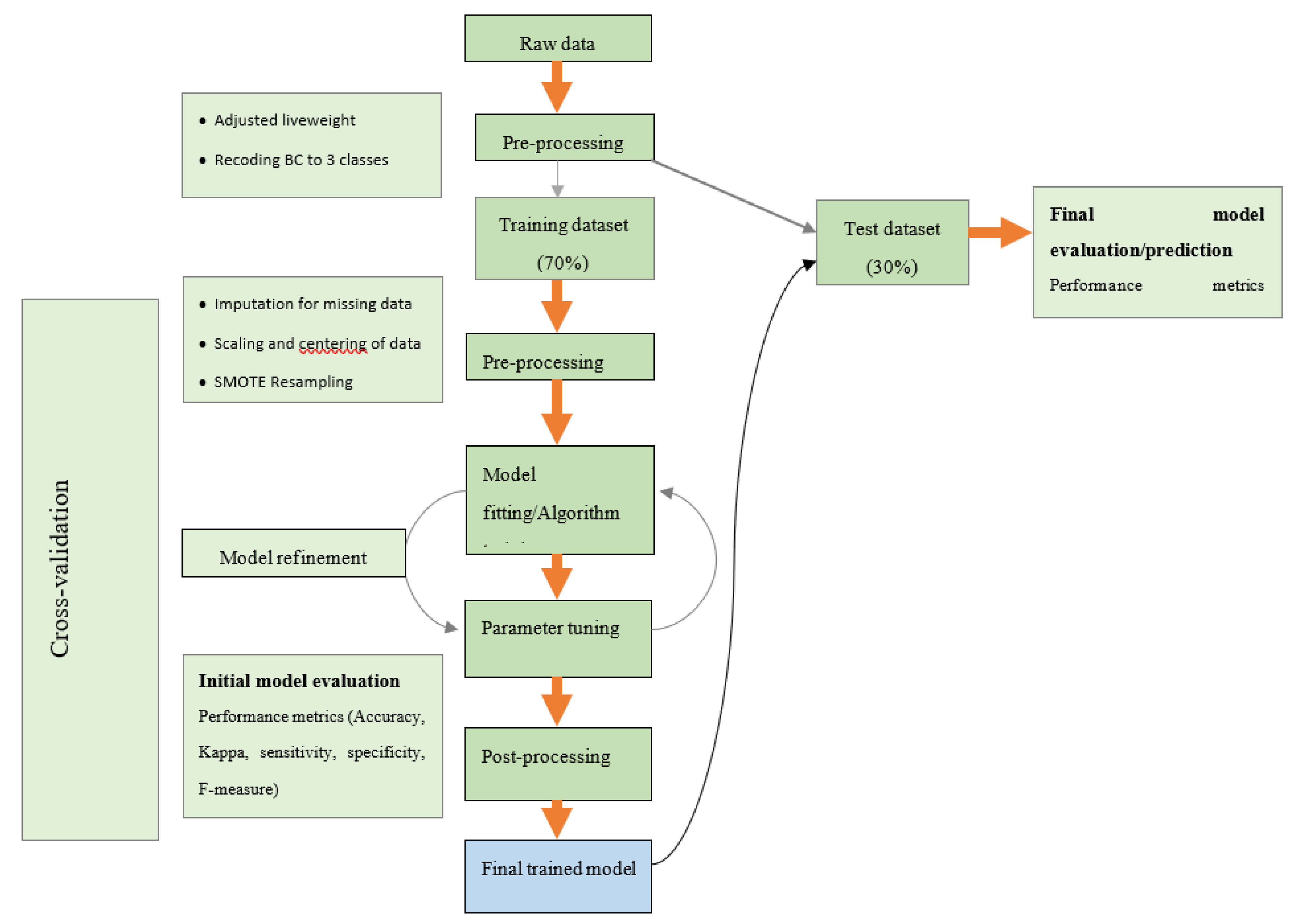
2.2.1. Variable Selection and Model Building

The best variable combinations for prediction of BCS (1, 2 or 3) at each stage of the annual cycle using liveweight were selected through the regularization and variable selection technique utilizing the elastic net method in the glmnet extension [27] in the caret package [21]. The elastic net method combines the power of two penalized-regularization methods (ridge and lasso regression) to search for significant predictors and handling of collinearity [28].

All models were fitted and validated using four steps as described by Semakula et al. [9]. The steps included: (i) data partitioning, (ii) resampling, (iii) model training and (iv) validation. Data were partitioned with stratification into training and testing datasets in a ratio of 3:1, with replacement. Resampling was done using the bootstrapping and aggregation [29] procedures in the caret package [21]. During resampling, 10 equal-sized subsamples, repeated three times, were selected from the dataset. Prediction models were trained on nine subsample sets which were used to compute the parameters, and the 10th was used to evaluate the model as well as compute the error. The procedure was run 30 times (10-folds repeated three times), and the average parameter values and their probabilities were computed as described by Semakula et al. [9].

The algorithms used for this work were selected from a range of probabilistic and nonprobabilistic methods in order to cover the most commonly used machine learning algorithms [17,30]. A summary of the concepts, advantages and disadvantages of each algorithm is given in

Table A1. Key model performance characteristics of common machine learning algorithms (selecting the most appropriate algorithms).

Model 1	Concept 2	Parameter and Processes Required 3	Sample Size and Data Dimensionality	Assumptions and Data Requirements	Covariate Pools 4	Computational Time	Interpretability 5	Prone to Overfitting	References
Ordinal	Probabilistic regression	No hyperparameters	Affected by small sample sizes	proportional odds, linearity	No	Fast	White box	Yes	[32,56,58]
Multinom	Probabilistic regression	No hyperparameters	Yes	proportional odds, linearity	No	Fast	White box	Yes	[32,58,61]
LDA	Dimension reduction + separability between classes	No hyperparameters	Affected by small sample sizes, Good for high dimension data	Normality, linearity & continuous independent variables	No	Fast	White box	Yes	[62,63,64]
CART	Decision trees and regression	Hyperparameters	Performs well with large datasets	numerical or categorical outcome	can remove redundant covariates	Fast	Low-level black box	No	[65,66]
RF	Decision trees, regression and bugging	Up to three hyperparameters	Performs well on small & high dimensionality data	numerical or categorical outcome	can remove redundant covariates	Decreases with sample size	Low-level black box	No	[17,67]
XGB	Regression trees + gradient boosting	Hyperparameter	Require large datasets	numerical or categorical outcome	can remove redundant covariates	Very fast	High-level black box	Yes, if large number of trees	[68,69]
K-NN	Regression curve + hyperparameter (k)	One hyperparameter	Not good for large & high dimensionality data	No assumptions but requires scaled data	No	Decreases with sample size	Fairly interpretable	Yes	[17,70]
SVM	Maximal margins + kennel functions	Two hyperparameters	Not good for high dimension data	No assumptions	No	Decreases with sample size	High-level black box	Yes	[71,72]
ANN	Nodes (artificial neurons)	Up to seven hyperparameters	Sensitive to sample size and data dimensionality	numerical or categorical outcome	No	computationally very expensive and time consuming	High-level black box	Yes	[73]

¹ Model (Ordinal: ordinal logistic regression, multinorm: multinomial regression, LDA: linear discriminant analysis, CART: classification and regression tree, RF: random forest, XGB: Gradient boosting decision trees model, K-NN: k-nearest neighbors, SVM: support vector machines, ANN: neural networks). ² Concept: How the algorithm works. ³ Parameter and processes: Tuning parameters for the algorithm. ⁴ Covariate pools: Intrinsic ability to remove redundant variables or to select important variables. ⁵ Interpretability: White box: clear model structure with parameters: black boxes: model structure and the relationship between variables is unknown. NB: The criteria used to summarize the key model performance characteristic was a modified version of a 5-point criteria by Khaledian and Miller [17].

in Appendix A. Further, the criteria for selecting these methods included (i) successful application in other animal science studies [16,19,20] and (ii) ability to handle multiclass categorization [24]. Three traditional (ordinal logistic, multinomial regression [31,32] and linear discriminant analysis (LDA) [33]) statistical models (white box or low-level machine learning models), two low-level black models (random forest (RF) [34] and classification and regression trees (CART) [35]) and four high-level black box models (support vector machines (SVM) [36] and k-nearest neighbors (K-NN) [37,38], neural networks (ANN), and gradient boosting decision trees (XGB) [39]) were compared. Machine learning models can be categorized in two main ways: (i) whether data provides labels that classify variables (supervised) or not (unsupervised) [40]; and (ii) if a clear description of the analysis detailing how covariates and the target variable are related (classical statistical methods or white boxes), a partial description blue print (low-level or semiblack boxes) or no description can be given (high-level black boxes) [17]. All algorithms were implemented in R package using several caret package extensions (nnet, multinom, polr, lda, rpart, svmLinear, xgblinear, rf and knn (http://topepo.github.io/caret/index.html, accessed on 19 January 2021)). A chart summarizing the model building and evaluation procedures is given as in the appendices (Figure A1).

2.2.2. Model Performance Evaluation

Using a three-class BCS scale (1.0–2.0, 2.5–3.5, >3.5), model fit and ranking between models were assessed using overall accuracy, balanced accuracy, precision, F-measure, sensitivity, and specificity. The metrics were computed from the number of true positive (TP), true negative (TN), false positive (FP) and false negative (FN) predictions as described by Tharwat [24]. In addition, Cohen’s kappa statistic [41]—a common measure to calculate agreement between the classification of qualitative observations was calculated as described by McHugh [42] and Botchkarev [43]. To evaluate the power of the algorithms to correctly classify ewe BCS, measures of the balance (authenticity and prediction power) between sensitivity and specificity were computed. These indicators of model power and authenticity (positive likelihood ratio, negative likelihood ratio and Youden’s index) combine sensitivity and specificity to emphasize how well a model can predict the outcome [44]. A detailed description of the metrics (accuracy and authenticity) used in model assessment is given in

Table 1. Model performance evaluation metrics.

Model	Definition	Formula
Balanced accuracy	The proportion of correctly classified subjects for each class. Useful especially when there is class imbalance.	$\mathrm{Accuracy}=\frac{\frac{\mathrm{TP}}{\mathrm{TP}+\mathrm{FN}}+\frac{\mathrm{TN}}{\mathrm{TN}+\mathrm{FP}}}{2}$
Precision	The proportion of correctly classified subjects for a given class given that they truly belonged to that class	$\mathrm{Precision}=\frac{\mathrm{TP}}{\mathrm{TP}+\mathrm{FP}}$
F-measure	The harmonic mean of the precision and sensitivity best if there is some sort of balance between precision and sensitivity.	$\mathrm{F}-\mathrm{measure}=\frac{2 \ast \left(\mathrm{sensitivity} \ast \mathrm{precision}\right)}{\mathrm{sensitivity}+\mathrm{precision}}$
Sensitivity	The proportion of correctly classified subjects for a given class to those who truly belong to that class.	$\mathrm{Sensitivity}=\frac{\mathrm{TP}}{\mathrm{TP}+\mathrm{FN}}$
Specificity	The proportion of subjects correctly classified as not belonging to a given class to those that truly do not belong to that class.	$\mathrm{Specificity}=\frac{\mathrm{TN}}{\mathrm{TN}+\mathrm{FP}}$
Positive likelihood rate (PLR)	The ratio between the true positive and the false positive rates for “positive” events that are detected by a model.	$\mathrm{PLR}=\frac{\mathrm{Sensitivity}}{1-\mathrm{Specificity}}$
Negative likelihood rate (NLR)	The ratio between the false negative and true negative rates and mirrors the probability for “negative” events to be detected by a model.	$\mathrm{NLR}=\frac{1-\mathrm{Sensitivity}}{\mathrm{Specificity}}$
Youden’s index (YI)	The sum of sensitivity and specificity minus one	$\mathrm{YI}=\left(\mathrm{Sensitivity}+\mathrm{Specificity}\right)-1$
Cohen’s kappa (κ)	Measures the degree of agreement between two raters or ratings (inter-rater or interrater reliability)	κ $=\frac{p_o-p_e}{1-p_e}$

Where: TP = true positive, TN = true negative, FP = false positive, FN = false negative, κ = Cohen’s kappa statistic, p_o = actual observed agreement, and p_e represents chance agreement.

.

The analysis generated a dataset of 108 records (4 time points, 3 BCS classes and 9 models of two groups of model performance evaluation metrics firstly, the indicators of accuracy: balance accuracy, precision and F-measure, and secondly measures of model authenticity: sensitivity and specificity). To obtain a holistic picture of the overall model performance, the two groups of performance metrics were examined. Initially, each group of variables was explored using principal component analysis (PCA) to determine the appropriate number of components of dimensions where the Eigen values associated with each component were compared with those generated through a probabilistic process based on Monte Carol PCA for parallel analysis simulation [45,46]. Monte Carlo PCA simulated Eigen values allow comparisons based on the same sample size and number of variables. If the Eigen value of a component from real data is greater than the simulated one, then that component is important. Otherwise, if equal to or less than, such components are considered not important. Consequently, one component was considered important from each group of variables (indicators of accuracy: explained variance = 87%; indicators of sensitivity–specificity: explained variance = 61%) having explained most of the variability in the group data.

Principal component analysis is limited to continuous data. In order to decipher the patterns in the relationship between the categorical variable (BCS) and each model regarding their overall performance, a correspondence analysis was required. Therefore, the FAMD function in the FactoMiner package [47] was used to analyze both groups of variables. The FAMD extension combines PCA and multiple correspondence analysis (MCA) to conduct factor analysis. Each group of variables then resulted in a single dimension (latent variable). A scatterplot of accuracy and sensitivity–specificity latent variables was constructed for each of the four stages of the annual sheep weighing cycle. Models were ranked on a scale of 1 to 9 (where 1 is best and 9 is the poorest) at each stage of the annual cycle, to obtain the overall performance rank.

3. Results

3.1. Overall Performance of Machine Learning Models

This section presents results for the accuracy in a broad sense, sensitivity and specificity of nine models in predicting ewe BCS based on the testing dataset (

Table 2. Accuracy and kappa statistics of nine predictive models for ewe BCS at 43–54 months of age at different stages of the annual cycle. Values in parenthesis denote the minimum and maximum accuracy, in ascending order.

	Pre-Breeding		Pregnancy Diagnosis		Pre-Lambing		Weaning
Model	Accuracy	Kappa (κ)	Accuracy	Kappa (κ)	Accuracy	Kappa (κ)	Accuracy	Kappa (κ)
XGB	89.5(85.6–97.5) 3,1	79.6	91.2(88.5–93.4) 3,1	82.3	90.6(88.8–91.4) 2,1	82.9	91.7(90.1–93.2) 1,3	83.4
RF	89.0(84.7–96.6) 2,1	78.0	90.0(87.5–92.9) 3,1	78.0	89.2(86.6–91.6) 2,3	78.5	88.6(88.2–89.6) 1,3	77.1
K-NN	87.0(81.2–95.7) 2,1	75.5	86.8(84.7–89.8) 3,1	75.5	86.2(83.0–89.7) 2,3	66.0	86.4(84.6–88.8) 2,3	77.7
SVM	86.7(78.8–96.6) 2,1	75.9	88.5(84.8–93.1) 2,1	73.7	73.8(72.0–74.7) 2,1	71.7	88.8(85.3–91.2) 2,3	72.7
ANN	85.2(79.0–94.2) 2,1	72.2	82.0(80.5–85.1) 2,1	65.6	78.9(75.5–82.4) 1,3	69.5	84.0(82.0–86.9) 1,3	68.0
Multinorm	82.7(76.4–91.7) 2,1	66.8	77.6(73.8–80.0) 3,1	56.1	73.5(71.8–75.1) 1,3	48.8	75.9(74.4–78.1) 3,2	51.8
LDA	81.2(73.8–91.1) 2,1	63.6	77.1(72.2–79.6) 3,1	54.6	73.8(71.5–75.5) 1,3	49.5	75.9(74.4–78.7) 1,2	51.7
Ordinal	79.6(70.7–88.4) 2,1	48.4	72.7(67.6–75.8) 2,1	47.7	68.4(58.7–74.8) 2,3	37.0	72.4(67.8–76.2) 2,1	44.9
CART	72.6(58.6–85.1) 2,1	47.3	69.8(64.0–73.3) 3,1	40.5	67.5(62.8–71.1) 1,2	41.8	66.6(61.4–70.1) 2,1	33.2

Model: (XGB: Gradient boosting decision trees model, RF: random forest, K-NN: k-nearest neighbors, SVM: support vector machines, ANN: neural networks, Multinorm: multinomial regression, LDA: linear discriminant analysis, Ordinal: ordinal logistic regression, CART: classification and regression tree). The superscripts ^1,2,3 where 1: 1.0–2.0, 2: 2.5–3.5 and 3: >3.5 indicate the BCS class from which the value was observed. The first superscript indicates the class from which the minimum estimate was observed, while the second value indicates the class from which the maximum estimate was achieved). All models were significant (p < 0.05) and better than a random guess (i.e., accuracy = 33.3%). All ewe BCS predictions were based on current and previous liveweight.

and

Table 3. Indicators of authenticity (sensitivity and specificity) of nine predictive models for ewe BCS at 43–54 months of age at different stages of the annual cycle. Values in parenthesis denote the minimum and maximum sensitivity or specificity, in ascending order.

	Pre-Breeding		Pregnancy Diagnosis		Pre-Lambing		Weaning
Model	Sensitivity	Specificity	Sensitivity	Specificity	Sensitivity	Specificity	Sensitivity	Specificity
XGB	86.0(79.7–96.3) 3,1	93.1(89.1–98.9) 2,1	88.2(83.7–90.4) 3,1	94.2(93.1–96.3) 2,1	87.5(85.9–88.8) 1,3	93.8(89.7–97.5) 2,1	89.0(84.8–92.3) 1,2	94.5(91.6–96.5) 2,3
RF	85.3(80.0–95.3) 2,1	92.8(89.3–97.9) 2,1	86.7(80.9–90.3) 3,1	93.4(90.5–95.5) 2,1	85.6(82.6–88.6) 1,3	92.8(87.5–96.4) 2,1	84.8(82.5–87.6) 1,2	92.4(88.9–93.4) 2,3
SVM	82.6(74.8–93.8) 2,1	91.4(87.5–97.5) 2,3	82.3(75.3–84.2) 3,2	91.2(84.2–95.4) 2,1	81.5(73.5–86.1) 1,3	90.8(81.1–98.1) 2,1	81.9(77.6–85.6) 3,2	90.9(83.5–95.1) 2,3
K-NN	82.2(66.8–96.2) 2,1	91.2(85.9–97.0) 3,1	84.7(75.5–91.8) 2,1	92.3(88.4–94.5) 3,1	65.0(63.0–67.3) 1,2	82.5(76.8–86.4) 2,1	85.1(78.6–88.9) 2,3	92.6(91.9–93.6) 2,3
ANN	80.2(71.3–91.7) 2,1	90.2(86.7–96.7) 2,1	76.0(73.2–78.0) 3,1	88.0(84.3–92.2) 2,1	71.8(56.5–80.2) 1,3	85.9(78.8–94.4) 2,1	78.7(70.5–84.1) 1,2	89.3(82.4–93.5) 2,1
Multinom	76.8(68.5–89.0) 2,1	88.5(84.4–94.5) 2,1	70.0(62.7–71.4) 3,2	85.1(81.8–88.7) 2,1	64.7(58.6–68.7) 1,3	82.4(80.6–84.9) 2,1	67.9(63.3–76.2) 3,1	83.9(80.1–86.2) 2,1
LDA	74.9(64.7–87.7) 2,1	87.6(82.8–94.4) 2,1	69.4(57.1–82.7) 3,2	84.8(76.6–90.7) 2,1	65.0(56.3–69.4) 1,3	82.5(79.2–86.8) 2,1	67.8(61.5–79.8) 3,2	83.9(77.6–87.4) 2,3
Ordinal	72.7(61.6–82.4) 2,1	86.5(79.7–94.5) 2,1	63.6(60.7–67.9) 2,3	81.7(73.1–90.9) 2,1	57.9(41.4–69.3) 2,3	79.0(76.1–80.8) 2,1	63.2(58.3–68.5) 3,1	81.6(72.8–88.2) 2,3
CART	63.3(37.0–82.5) 2,1	81.9(77.6–87.8) 3,1	59.7(41.1–77.3) 3,2	80.0(67.1–86.0) 2,3	56.7(37.9–72.3) 1,2	78.3(71.2–87.7) 2,1	55.4(39.2–62.9) 2,1	77.7(72.4–83.6) 3,2

Model: (XGB: Gradient boosting decision trees model, RF: random forest, K-NN: k-nearest neighbors, SVM: support vector machines, ANN: neural networks, Multinorm: multinomial regression, LDA: linear discriminant analysis, Ordinal: ordinal logistic regression, CART: classification and regression tree). The superscripts ^1,2,3 where 1: 1.0–2.0, 2: 2.5–3.5 and 3: > 3.5 indicate the BCS class from which the value was observed. In their sequence, the first superscript indicates the class from which the minimum estimate was observed, while the second value indicates the class from which the maximum estimate was achieved). All ewe BCS predictions were based on current and previous liveweight.

). Additionally,

Table A2. A pairwise comparison (Bonferroni p-value adjustment) of overall performance accuracy of nine predictive models for BCS, at different stages of the annual cycle (PB: pre-breeding, PD: pregnancy diagnosis, PL: pre-lambing, W: weaning) in 43–54-month-old ewes. p-value > 0.05 indicates no significant difference between models. All ewe BCS predictions were based on liveweight record 2.

Model A	Model B	PB	PD	PL	W
XGB	K-NN	0.011	0.000	0.000	0.000
	RF	1.000	0.000	0.245	0.007
	SVM	0.010	0.000	0.000	0.000
	ANN	0.000	0.000	0.001	0.000
	Multinorm	0.000	0.000	0.000	0.000
	LDA	0.000	0.000	0.000	0.000
	Ordinal	0.000	0.000	0.000	0.000
	CART	0.000	0.000	0.000	0.000
K-NN	RF	0.003	0.281	0.000	0.041
	SVM	1.000	1.000	0.000	1.000
	ANN	0.231	0.000	1.000	0.000
	Multinorm	0.000	0.000	0.779	0.000
	LDA	0.000	0.000	1.000	0.000
	Ordinal	0.000	0.000	0.000	0.000
	CART	0.000	0.000	0.004	0.000
RF	SVM	0.203	0.014	0.008	0.002
	ANN	0.002	0.000	0.002	0.000
	Multinorm	0.000	0.000	0.000	0.000
	LDA	0.000	0.000	0.000	0.000
	Ordinal	0.000	0.000	0.000	0.000
	CART	0.000	0.000	0.000	0.000
SVM	ANN	0.563	0.000	0.021	0.000
	Multinorm	0.000	0.000	0.000	0.000
	LDA	0.000	0.000	0.000	0.000
	Ordinal	0.000	0.000	0.000	0.000
	CART	0.000	0.000	0.000	0.000
ANN	Multinorm	0.002	0.000	1.000	0.000
	LDA	0.000	0.000	1.000	0.000
	Ordinal	0.002	0.000	0.000	0.000
	CART	0.000	0.000	0.903	0.000
Multinorm	LDA	0.019	1.000	1.000	1.000
	Ordinal	0.004	0.000	0.000	0.000
	CART	0.000	0.000	0.023	0.000
LDA	Ordinal	0.019	0.000	1.000	0.006
	CART	0.000	0.000	0.032	0.000
Ordinal	CART	0.000	0.002	0.047	0.008

Model: (XGB: Gradient boosting decision tree model, RF: random forest, K-NN: k-nearest neighbors, SVM: support vector machines, ANN: neural networks, multinorm: multinomial regression, LDA: linear discriminant analysis, Ordinal: ordinal logistic regression, CART: classification and regression tree).

is supplied in the appendix, which show the comparisons between model accuracy across stages of the annual sheep weighing cycle in New Zealand.

Results showed that there were significant (p < 0.05) differences in model prediction performance based on the Boniferroni p-value adjustment method for pairwise comparisons (Table A2, Appendix A). The gradient boosting decision tree algorithm (XGB) had the highest (p < 0.05) accuracy (average = 90.3%) and kappa statistic (κ = 82.1%) at pre-breeding, pregnancy diagnosis, pre-lambing and weaning, making it the most accurate algorithm for ewe BCS prediction on the one to three (1.0–2.0; 2.5–3.5; >3.5) scale (Table 2). The RF (Figure A2, Appendix A) algorithm had a slightly lower but still good accuracy, making it the best alternative to XGB. The multinorm, LDA, ordinal and CART algorithms had moderate to fair accuracies. Pre-lambing, XGB and RF were comparable and had the highest accuracies. The random forest and k-nearest neighbors (K-NN) in decreasing order were also considered good prediction models, having scored above 80% accuracy and 70% kappa statistics at all times of the year. The CART algorithm consistently gave the lowest (p > 0.05) accuracy except pre-lambing where its accuracy was (p = 0.047; Table A1) comparable to that of ordinal logistic regression. The lowest average accuracy was 66.6% seen for the CART model at weaning (Table 2, parenthesis). Overall, all algorithms had greater accuracy than a random guess (i.e., accuracy = 33.3%) in classifying BCS.

In terms of overall authenticity, models were biased towards being more specific than sensitive (Table 3). The ranking of model authenticity followed a trend like that of accuracy. The gradient boosting decision tree algorithm (XGB) had the highest sensitivity (average = 87.7%) as well as specificity (average = 93.9%) across all stages of the annual sheep weighing cycle, making it the most authentic and powerful algorithm for categorizing ewe into the correct BCS classes on three-point scale (1.0–2.0; 2.5–3.5; >3.5) (Table 3). The XGB model was closely followed by RF (average sensitivity = 85.5%, average specificity: 92.8%) while CART (average sensitivity: 58.7%, average specificity: 79.5%) was the poorest.

In the following section we present results for the construct or latent variables which are representative of the three specific measures of model accuracy (class-level or balanced accuracy, precision and F-measure) together with two indicators of predictive power/authenticity (sensitivity, specificity) across four stages of the annual sheep weighing cycles (Figure 2, Figure 3, Figure 4 and Figure 5). A summary of the indicators of accuracy and authenticity was provided in Table 2 and Table 3. Additionally,

Table A3. Accuracy measures (precision, F-measure) of nine predictive models for ewe BCS at 43–54 months of age pre-breeding at different stages of the annual sheep weighing cycle (PB: pre-breeding, PD: pregnancy diagnosis, PL: pre-lambing and W: weaning). Values in parenthesis indicate the minimum and maximum.

	PB		PD		PL		W
Model	Precision %	F-Measure %	Precision %	F-Measure %	Precision %	F-Measure %	Precision %	F-Measure %
XGB	86.1(78.2–97.7)	86.0(80.1–96.9)	87.9(80.8–94.5)	87.6(84.1–90.0)	87.9(80.8–94.5)	87.6(84.1–90.0)	89.1(84.2–92.8)	89.0(87.5–91.3)
RF	85.3(78.1–95.9)	85.3(79.0–95.6)	86.9(83.2–91.1)	86.7(83.6–90.7)	86.1(77.0–91.7)	85.7(81.0–89.0)	84.9(79.3–88.8)	84.7(83.2–86.4)
SVM	82.7(74.1–95.1)	82.7(74.5–94.4)	83.4(74.6–90.3)	82.6(80.0–87.2)	83.5(68.7–95.0)	81.8(76.0–86.4)	82.8(71.6–89.4)	82.0(78.0–85.7)
K-NN	82.3(75.0–94.4)	82.0(71.8–95.3)	84.7(77.5–89.5)	84.5(80.9–90.6)	64.5(58.1–68.6)	64.1(61.8–65.5)	84.9(79.3–88.8)	85.1(80.5–88.1)
ANN	80.3(71.9–93.4)	80.3(71.6–92.6)	76.3(72.1–83.7)	76.1(73.2–80.7)	73.5(64.5–83.3)	71.5(67.4–76.2)	79.5(70.0–85.0)	78.7(76.4–82.6)
Multinom	76.8(67.7–89.3)	76.8(68.1–89.1)	70.2(65.6–76.4)	70.0(64.1–73.8)	64.8(62.8–65.9)	64.6(62.1–67.1)	68.1(65.0–70.7)	67.7(65.7–70.2)
LDA	75.0(64.3–89.0)	74.9(64.5–88.3)	70.5(65.1–79.0)	69.3(61.8–73.3)	65.3(61.9–67.9)	64.9(61.5–67.7)	68.3(63.4–70.8)	67.6(65.8–70.7)
Ordinal	73.2(59.2–88.5)	72.9(60.4–85.3)	64.9(55.0–77.4)	63.8(58.4–68.1)	57.3(45.8–64.2)	57.5(43.5–66.7)	64.2(52.9–70.9)	63.4(57.4–68.7)
CART	62.1(47.3–77.7)	62.3(41.5–80.0)	61.1(55.5–68.9)	59.2(48.5–64.6)	57.3(55.1–60.5)	55.7(46.6–62.5)	55.4(53.4–59.0)	54.8(45.3–60.9)

Model: (XGB: Gradient boosting decision tree model, RF: random forest, K-NN: k-nearest neighbors, SVM: support vector machines, ANN: neural networks, multinorm: multinomial regression, LDA: linear discriminant analysis, Ordinal: ordinal logistic regression, CART: classification and regression tree).

provides two extra measures of accuracy (precision and F-measure) used in the construction of the accuracy latent variable. The results show the patterns in the relationship between the latent variables with BCS class prediction for each model. The CART model had the lowest accuracy and power measures across all stages of the annual sheep weighing cycle and was selected as the reference for comparisons.

3.1.1. Pre-Breeding

At pre-breeding, the models had a clear-cut hierarchy in performance, with XGB being the best and CART the poorest (Figure 2). The XGB was the best algorithm with 17% more accuracy than CART, which was the least accurate in predicting ewe BCS (Table 2). The best balance between accuracy and authenticity (points along or touching the diagonal line) was observed in the moderate performing models including ANN, multinom, LDA and ordinal (Figure 2). The best performing models (XGB, RF, SVM and K-NN) were biased towards accuracy while the poorest (CART) was biased towards authenticity. In terms of BCS, the best accuracy was achieved in the 1.0–2.0 class and the lowest in the 2.5–3.5 class for all models except for XGB which was least accurate in the >3.5 class. The best accuracy (97.5%) was achieved using the XGB in the 1.0–2.0 BCS class, and the lowest (58.6%) was observed using the CART algorithm in the 2.5–3.5 class (Table 2, parenthesis).

All models were most sensitive to the 1.0–2.0 class and least sensitive to the 2.5–3.5 class except XGB which was least sensitive to the > 3.5 class. The XGB was the best algorithm, being 23% more sensitive than CART, which was the least sensitive in predicting ewe BCS (Table 3). The highest BCS classification sensitivity was observed using XGB and K-NN models (96.3%) in the 1.0–2.0 BCS class while CART (37.0%) had the lowest in the 2.5–3.5 class (Table 3, parenthesis). All models had the highest specificity observed in the 1.0–2.0 BCS class except for SVM which had the highest specificity in the >3.5 class and both K-NN and CART which had their lowest in the >3.5 class. The XGB was the best algorithm with 12% more specificity than CART, which had the least specificity in predicting ewe BCS (Table 2). The highest specificity (98.9%) was observed in the 1.0–2.0 class for XGB and the lowest (72.6%) in the >3.5 class for CART model (Table 3, parenthesis).

3.1.2. Pregnancy Diagnosis

At pregnancy diagnosis, the models had a clear-cut hierarchy in performance, with XGB being the best and CART the poorest (Figure 3). The multinom and LDA models were closely juxtaposed indicating that they had comparable performance. The XGB was the best algorithm with 21% more accuracy than CART, which was the least accurate in predicting ewe BCS (Table 2). The best balance between accuracy and authenticity was observed in the ANN model. The XGB, RF, SVM and K-NN models were biased towards accuracy while the multinom, LDA, ordinal and CART were biased towards authenticity (Figure 3). In terms of BCS, the best accuracy was achieved in the 1.0–2.0 class and the lowest in the >3.5 class for all models except for SVM, ANN and ordinal which were least accurate in the 2.5–3.5 class. The highest accuracy (93.4%) was achieved using the XGB in the 1.0–2.0 BCS class and the lowest (64.0%) was observed using the CART algorithm in either the >3.5 class (Table 2, parenthesis).

There was no clear pattern in class-level model sensitivity at pregnancy diagnosis. The XGB was the best algorithm with 29% more sensitivity than CART, which was the least sensitive in predicting ewe BCS (Table 3). The highest BCS classification sensitivity was observed using K-NN models (91.8%) in the 1.0–2.0 BCS class while CART (41.1%) had the lowest in the >3.5 class (Table 3, parenthesis). All models had the highest specificity observed in the 1.0–2.0 BCS class except for CART which had the its highest in the >3.5 class. The XGB was the best algorithm with 14% more specificity than CART, which had the least specificity in predicting ewe BCS (Table 2). The highest specificity (96.3%) was observed in the 1.0–2.0 class for XGB and the lowest (67.1%) in the 2.5–3.5 class for CART model.

3.1.3. Pre-Lambing

At pre-lambing, the models had a clear-cut hierarchy in performance, with XGB being the best and CART the poorest (Figure 4). It was worth noting that the K-NN model, which had been among the best four models at pre-breeding and pregnancy diagnosis, was downgraded into a moderate model. The K-NN, multinom and LDA models had overlapping overall performance. The XGB was the best algorithm with 23% more accuracy than CART, which was the least accurate in predicting ewe BCS (Table 2). All models were biased with XGB, RF, SVM and ANN inclined towards accuracy, while K-NN, Multinon, LDA, ordinal and CART were inclined towards authenticity (Figure 4). The best overall accuracy was achieved in the >3.5 BCS class and the lowest in the 2.5–3.5 class (Table 2, parenthesis). Regarding BCS class-level model accuracy, there was no clear pattern. The majority of the models (RF, K-NN, ANN, multinom, LDA and ordinal) were most accurate in the >3.5 BCS class and least accurate in the 2.5–3.5 class. The least accuracy for majority of the models (XGB, RF, K-NN, SVM and ordinal) was observed in the 2.5–3.5 class. The highest accuracy (92%) was achieved using the RF model in the >3.5 BCS class and the lowest (63%) was observed using the CART algorithm in either the 1.0–2.0 class (Table 2, parenthesis).

All models were most sensitive to the >3.5 class and least sensitive to the 1.0–2.0 class except K-NN and CART with the highest sensitivity in the 2.5–3.5 class and ordinal with the lowest sensitivity in the 2.5–3.5 class. The XGB was the best algorithm with 31% more sensitive than CART, which was the least sensitive in predicting ewe BCS (Table 3). The highest BCS classification sensitivity was observed using XGB models (88.8%) in the >3.5 BCS class while CHART (37.9%) had the lowest in the 1.0–2.0 class (Table 3, parenthesis). All models had the highest specificity observed in the 1.0–2.0 BCS class. The XGB was the best algorithm with 16% more specificity than CART, which had the least specificity in predicting ewe BCS (Table 2). The highest specificity (97.5%) was observed in the 1.0–2.0 class for XGB and the lowest (71.2%) in the 2.5–3.5 class for CART model (Table 3, parenthesis).

3.1.4. Weaning

At weaning, the models had a clear-cut hierarchy in performance, with XGB being the best and CART the poorest (Figure 5). The RF and K-NN models had overlapping overall performance. The XGB was the best algorithm with 33% more accuracy than CART, which was the least accurate in predicting ewe BCS (Table 2). The majority of the models were biased towards accuracy, except for multinom, LDA, ordinal and CART, which were inclined towards authenticity (Figure 5). The best overall accuracy was achieved in the >3.5 BCS class and the lowest in the 2.5–3.5 class. Regarding the BCS level model accuracy, there was no clear pattern. However, the majority of the models (XGB, RF, SVM, K-NN and ANN) were most accurate in the >3.5 BCS class. The least model accuracy was equally observed in the 1.0–2.0 and 2.5–3.5 BCS classes, across models. The highest accuracy (93.2%) was achieved using the RF model in the >3.5 BCS class, and the lowest (61.4%) was observed using the CART algorithm in either the 2.5–3.5 class (Table 2, parenthesis).

There was no clear pattern in class-level model sensitivity at weaning. The XGB was the best algorithm with 34% more sensitivity than CART, which was the least sensitive in predicting ewe BCS (Table 2). The highest BCS classification sensitivity was observed using XGB models (92.3%) in the 2.5–3.5 BCS class while CHART (39.2%) had the lowest in the 2.5–3.5 class (Table 3, parenthesis). All models had the highest specificity observed in the >3.5 BCS class and the least in the 2.5–3.5 class, except for the CART, whose specificity arrangement was the opposite, and for ANN and multinom, which had their highest specificity in the 1.0–2.0 class. The XGB was the best algorithm with 17% more specificity than CART, which had the least specificity in predicting ewe BCS (Table 3). The highest specificity (96.5%) was observed in the 1.0–2.0 class for XGB and the lowest (72.4%) in the 2.5–3.5 class for CART model (Table 3, parenthesis).

3.1.5. The Balance between Sensitivity and Specificity

The data showed that the overall specificity 86% (67–98%) was higher than sensitivity 74% (37–96%) values across all algorithms (Table 3). An assessment of the indicators of the balance between sensitivity and specificity was undertaken and the indices are summarized in

Table 4. Measures of the balance between sensitivity and specificity of the BCS prediction models by stage of the annual cycle.

	Pre-Breeding			Pregnancy Diagnosis			Pre-Lambing			Weaning
Model	PLR	NLR	YI	PLR	NLR	YI	PLR	NLR	YI	PLR	NLR	YI
XGB	33.41	0.15	0.79	16.48	0.13	0.82	19.39	0.13	0.81	18.32	0.12	0.83
RF	20.49	0.16	0.78	14.45	0.14	0.80	15.33	0.16	0.78	12.25	0.16	0.77
SVM	16.88	0.19	0.74	12.13	0.19	0.74	18.48	0.20	0.72	11.79	0.20	0.73
K-NN	15.21	0.20	0.73	12.3	0.17	0.77	3.90	0.42	0.48	11.64	0.16	0.78
ANN	13.04	0.22	0.70	6.94	0.27	0.64	6.32	0.32	0.58	8.66	0.24	0.68
Multinom	8.65	0.27	0.65	4.87	0.35	0.55	3.69	0.43	0.47	4.28	0.38	0.52
LDA	8.16	0.29	0.62	5.12	0.36	0.54	3.78	0.42	0.48	4.37	0.38	0.52
Ordinal	7.66	0.32	0.59	4.20	0.45	0.45	2.83	0.54	0.37	3.83	0.45	0.45
CART	3.92	0.46	0.45	3.27	0.49	0.40	2.70	0.54	0.35	2.49	0.57	0.33

Models: (XGB: Gradient boosting decision trees model, RF: random forest, K-NN: k-nearest neighbors, SVM: Support Vector Machine, ANN: neural networks, multinorm: multinomial regression, LDA: linear discriminant analysis, Ordinal: ordinal logistic regression, CART: classification and regression tree). Measures of the balance between sensitivity and specificity (PLR: Positive likelihood rate, NLR: Negative likelihood rate and YI: Youden’s index). A good model (PLR value > 1.0 and the larger PLR is the better, NLR value less than 1.0 and the smaller the better, YI ranges from 0 to 1.0 and values that approach 1.0 show higher authenticity and prediction power).

. The positive likelihood ratio (PLR) for all models were greater than 1.0 while the negative likelihood ratio (NLR) was less than 1.0 across stages of the annual cycle. The XGB model had the highest PLR and lowest NLR, while CART had the lowest PLR and highest NLR across stage of the annal cycle. Similarly, Youden’s index, YI, was consistently highest for XGB model and lowest for the CART model.

3.1.6. Overall Model Ranking

Overall, black box models were better than low-level white box models (

Table 5. Model ranking by stage of annual cycle and overall.

Model	Pre-Breeding	Pregnancy Diagnosis	Pre-Lambing	Weaning	Overall
XGB	1	1	1	1	1(1.0)
RF	3	2	2	2	2(2.3)
SVM	4	3	4	3	3(3.5)
K-NN	2	6	3	4	4(3.8)
ANN	5	4	5	5	5(4.8)
Miltinom	6	5	6	6	6(5.8)
LDA	7	7	7	7	7(7.0)
Ordinal	8	8	8	8	8(8.0)
CART	9	9	9	9	9(9.0)

Overall (overall rank with means in parenthesis). The lower the rank the greater the BCS prediction performance.

). The XGB was consistently the best performing while CART was the poorest model. There was change in model ranking across stages of the annual cycle except for XGB, LDA, ordinal and CART.

4. Discussion

The present study utilized machine learning classification algorithms to explore the possibility of predicting BCS from current and previous liveweight in mature ewes (at approximately 43–54 months of age). Body condition score was treated as a categorical variable with three levels (1.0–2.0, 2.5–3.5; >3.5). Nine of the most recognized machine learning models (XGB, ANN, RF, K-NN, SVM, ordinal, multinom, LDA and CART models) were applied to preprocessed datasets.

We applied a strategy to reduce the accuracy and authenticity measures into two dimensions in order to generate latent variables or constructs that were plotted to give a visual summary of model performance. This technique gave a visual display (a holistic picture) of overall model performance which made it easier to decipher the patterns in the relationship between the accuracy and authenticity of models in BCS prediction. Previous studies have suggested the use of several metrics to give an indication about a model’s accuracy and authenticity [24,43,48,49]. These have, however, been piecemeal with no unifying interface. By bringing together both accuracy and authenticity measures in a single display, we appear to have cracked that enigma. This innovation could serve as a platform for interrogating even better ways of model performance evaluation.

4.1. Overall Accuracy

The findings suggest that ewe BCS prediction from current and previous liveweight can be achieved using machine learning classification algorithms within the limited BCS range used in the present study. The results indicated that XGB was the most efficient and robust model (overall accuracy = 87.6%; sensitivity = 87.7%; specificity = 93.9%). Other good alternatives to XGB for predicting ewe BCS were three algorithms (K-NN, RF and SVM) with accuracies > 80% and kappas > 70%, while the remaining four (CART, ordinal, LDA and multinomial) were weak algorithms (accuracies < 70%, kappas < 60%). All models performed better than a random guess, with the most efficient models giving prediction errors as low as 11% and 38%. According to Galdi and Tagliaferri [50], a perfect classifier has a rate of 100%, while a random guess would give a 33.3% error for three-level classifiers [50,51]. The weakest algorithms outperformed a random guess by only 8, 11, 15 and 20%, respectively, using the current study data. Whereas accuracy measures can be interpreted arbitrarily, Cohen’s kappa statistic has been classified [42,52] into six different categories, no agreement (values ≤ 0), none to slight (0.01–0.20), fair (0.21–0.40), moderate (0.41–0.60), substantial (0.61–0.80) and almost perfect agreement (0.81–1.00). Further, Fleiss et al. [53] suggested that kappa values greater than 0.75 may be taken to represent excellent agreement beyond serendipity, values below 0.40 as poor agreement and values between 0.40 and 0.75 as fair to good agreement. The findings in this study suggest that using the top performing algorithms (XGB and RF), ewe BCS can be predicted with high accuracy across four phases of the annual cycle.

4.2. Class-Level Accuracy

Results also showed that at the accuracy-related class level, metrics including accuracy, precision and F-measure were highest for XGB, making it the most efficient and robust model for ewe BCS prediction. Further, there appeared to be variability in all metrics across stages of the annual sheep weighing cycle and BCS class. This variation in accuracy across the stages of the annual cycle suggests that with the exception of XGB, different models may be required to predict BCS at different stages of the annual cycle. Similarly, different models may be required if there is need for greater accuracy in one BCS class than others. This is especially important when great accuracy is required for management decisions with far reaching consequences such as when limited resources must be allocated to only target classes. Further, results indicated that the higher-level (black box) machine learning models such as XGB and RF were better at separating BCS into distinct classes than the lower-level (white box) models such as multinomial or ordinal logistic regression.

In the current study, the best balance between accuracy and authenticity (sensitivity–specificity) was achieved during pre-breeding compared to other stages of the annual cycle. This observation could have been due to the “relative ease” to condition score ewe pre-breeding than other stages of the annual cycle [2,54]. Prior to breeding, most farmers enhance ewe feeding in a process known as flushing [55,56], which likely resulted in uniform tissue (fat and muscle) distribution around the body. In addition, the weight measurements recorded pre-breeding are not confounded by the conceptus mass which is the case at pregnancy diagnosis and pre-lambing. The conceptus mass influences the ewe liveweight from pregnancy through the pre-lambing stage [54,57], which coincides with the two time-point weight measurements during those stages of the annual cycle. Further, during lactation a ewe has its greatest nutrient requirements for energy and protein [58], and at weaning a ewe is drained by the lactation process, leading to variability in fat deposition around the body; consequently, the ewe are lighter. Using the same ewe population, we have previously reported a decreasing trend in ewe BCS as a ewe aged, plateauing after 43–54 months [9]. This was attributed to a likelihood that farmers were underfeeding their aging ewes at certain stages or periods of the annual cycle. Lactation period could be one of such periods, resulting in failure to meet ewe dietary energy and protein requirements and consequently leading to thinner animals. The management conditions at pregnancy diagnosis, pre-lambing and weaning, therefore, could lead to differences in fat deposition around the body, resulting in variability in BCS.

4.3. Class-Level Model Authenticity

Among the indicators of model authenticity, the models had apparently greater specificity than sensitivity, which could point to unbalanced distinguishing power to make predictions. An examination of three indicators of balance between sensitivity and specificity or model authenticity/power (PLR and YI) indicated that all models had values within acceptable authenticity and power (PLR > 1.0, NLR < 1.0 and YI > 1.0) across stage four stages of the annual cycle, indicating that all models had balanced sensitivity and specificity. Results also showed that XGB had the highest PLR and YI and the lowest NLR. Combined with the results from the measures of accuracy, these results rank XBG as the most robust model for BCS prediction. Sensitivity is defined as the proportion of individuals or items who belong to a given BCS class and are correctly identified, while specificity is the proportion which do not belong to a given class and are excluded by the test. There exists an inverse relationship between sensitivity and specificity of a test or prediction model [59,60]. If a model has high sensitivity, it is capable of detecting “real” BCS classes, but it also faces losses from consuming more resources due to mandatory confirmatory tests (to rule out the false positives) or when the limited resources have to be given to only the right candidates. However, if a model has high specificity, the system benefits from a significant reduction in the consumption of resources and time, but it has a decreased capacity to detect “real” BCS classes, which can lead to failure to detect many events of importance [44]. The higher specificity would not be advantageous, as failure to detect ewes inside or outside the BCS range (2.5–3.5) for optimum productivity would affect management decisions negatively. Therefore, a good model needs to achieve a balance between sensitivity and specificity [55].

This study suggests that ewe BCS prediction from current and previous liveweight can usefully be achieved using machine learning classification algorithms within a limited BCS range used in the present study. This study used unadjusted liveweight (i.e., confounded by factors such as fleece length variations and fetal mass from pregnancy to lambing) records alone to achieve accuracies up to 89% in order to assign BCS to one out of three classes. It is likely that if adjusted liveweights were used together with other key variables that affect BCS, optimum accuracy would be achieved from these BCS prediction algorithms. Semakula et al. [10] suggested that the accuracy of BCS prediction could be improved if all key variables affecting the relationship between liveweight and BCS were accounted for. If this was the case, the efficiency of the machine learning models tested could also be enhanced.

Although not directly comparable, having used different scale ranges and different measures of model performance, the best ML model (XGB) in the current study had great efficiency (based on liveweight predictors, alone and achieved greater than 90% accuracies) and was stable (accuracy: 86–93%) across stages of the annual cycle. In their previous study based on linear regression models, Semakula et al. [10] achieved only weak to moderate wellness of fit (R² = 50%) using more resources (both LW and BCS records combined). Further, the model wellness of fit and accuracy varied greatly (R²: 28–64%) across stages of the annual cycle, making the linear regression models less stable. When combined, therefore, this suggests that machine learning models would offer better BCS predictions than the linear regression models.

5. Conclusions

The results of the present study showed that ewe BCS (grouped) can be predicted with great accuracy on a narrow BCS (1.0–2.0, 2.5–3.5, >3.5) scale from a ewe’s current and previous liveweight using machine learning algorithms. The gradient boosting decision trees algorithm was the most efficient for ewe BCS prediction. The results of this study, therefore, support the hypothesis that BCS can be accurately predicted from a ewe’s current and previous liveweights. The algorithms, having been trained on a large representative dataset, should be able to give accurate ewe BCS predictions. These algorithms (acquired intelligence) could be incorporated into weighing systems to easily and quickly give farmers ewe BCS without the need for the hands-on burden. Future studies should investigate how to ameliorate the accuracy of BCS prediction and the possibility of individual BCS prediction on a full range (1–5).

References

1. Jefferies, B. Body condition scoring and its use in management. Tasman. J. Agr. 1961, 32, 19–21. [Google Scholar]
2. Kenyon, P.R.; Maloney, S.K.; Blache, D. Review of sheep body condition score in relation to production characteristics. NZJ Agric. Res. 2014, 57, 38–64. [Google Scholar] [CrossRef]
3. Coates, D.B.; Penning, P. Measuring animal performance. In Field and Laboratory Methods for Grassland and Animal Production Research; Jones, L., Ed.; CABI Publishing: Wallingford, UK, 2000; pp. 353–402. [Google Scholar]
4. Morel, P.C.H.; Schreurs, N.M.; Corner-Thomas, R.A.; Greer, A.W.; Jenkinson, C.M.C.; Ridler, A.L.; Kenyon, P.R. Live weight and body composition associated with an increase in body condition score of mature ewes and the relationship to dietary energy requirements. Small Ruminant Res. 2016, 143, 8–14. [Google Scholar] [CrossRef]
5. Jones, A.; van Burgel, A.J.; Behrendt, R.; Curnow, M.; Gordon, D.J.; Oldham, C.M.; Rose, I.J.; Thompson, A.N. Evaluation of the impact of Lifetimewool on sheep producers. Anim. Prod. Sci. 2011, 51, 857–865. [Google Scholar] [CrossRef]
6. Corner-Thomas, R.A.; Kenyon, P.R.; Morris, S.T.; Ridler, A.L.; Hickson, R.E.; Greer, A.W.; Logan, C.M.; Blair, H.T. Brief communication: The use of farm-management tools by New Zealand sheep farmers: Changes with time. Proc. NZ Soc. Anim. Prod. 2016, 76, 78–80. [Google Scholar]
7. Besier, R.B.; Hopkins, D. Farmers’ estimations of sheep weights to calculate drench dose. J. Dept. Agr. West. Aust., Series 4 1989, 30, 120–121. [Google Scholar]
8. McHugh, N.; McGovern, F.M.; Creighton, P.; Pabiou, T.; McDermott, K.; Wall, E.; Berry, D.P. Mean difference in live-weight per incremental difference in body condition score estimated in multiple sheep breeds and crossbreds. Animal 2019, 13, 1–5. [Google Scholar] [CrossRef]
9. Semakula, J.; Corner-Thomas, R.A.; Morris, S.T.; Blair, H.T.; Kenyon, P.R. The Effect of Age, Stage of the Annual Production Cycle and Pregnancy-Rank on the Relationship between Liveweight and Body Condition Score in Extensively Managed Romney Ewes. Animals 2020, 10, 784. [Google Scholar] [CrossRef]
10. Semakula, J.; Corner-Thomas, R.A.; Morris, S.T.; Blair, H.T.; Kenyon, P.R. Predicting Ewe Body Condition Score Using Lifetime Liveweight and Liveweight Change, and Previous Body Condition Score Record. Animals 2020, 10, 1182. [Google Scholar] [CrossRef]
11. Bishop, P.A.; Herron, R.L. Use and misuse of the Likert item responses and other ordinal measures. Int. J. Exerc. Sci. 2015, 8, 297. [Google Scholar]
12. Blaikie, N. Analyzing Quantitative Data: From Description to Explanation; Sage: New York, NY, USA, 2003. [Google Scholar] [CrossRef] [Green Version]
13. Sullivan, G.M.; Artino, A.R. Analyzing and interpreting data from Likert-type scales. J. Grad. Med. Educ. 2013, 5, 541–542. [Google Scholar] [CrossRef] [Green Version]
14. Wicker, J.E. Applications of modern statistical methods to analysis of data in physical science. Ph.D. Thesis, University of Tennessee, Knoxville, TN, USA, May 2006. [Google Scholar]
15. Shahinfar, S.; Kahn, L. Machine learning approaches for early prediction of adult wool growth and quality in Australian Merino sheep. Comput. Electron. Agric. 2018, 148, 72–81. [Google Scholar] [CrossRef]
16. Shahinfar, S.; Kelman, K.; Kahn, L. Prediction of sheep carcass traits from early-life records using machine learning. Comput. Electron. Agric. 2019, 156, 159–177. [Google Scholar] [CrossRef]
17. Khaledian, Y.; Miller, B.A. Selecting appropriate machine learning methods for digital soil mapping. Appl. Math. Model. 2020, 81, 401–418. [Google Scholar] [CrossRef]
18. Morota, G.; Ventura, R.V.; Silva, F.F.; Koyama, M.; Fernando, S.C. Big data analytics and precision animal agriculture symposium: Machine learning and data mining advance predictive big data analysis in precision animal agriculture. Big data analysis in Animal Science 2018, 96, 1540–1550. [Google Scholar] [CrossRef] [PubMed]
19. Bakoev, S.; Getmantseva, L.; Kolosova, M.; Kostyunina, O.; Chartier, D.R.; Tatarinova, T.V. PigLeg: Prediction of swine phenotype using machine learning. PeerJ 2020, 8, e8764. [Google Scholar] [CrossRef]
20. R Core Team. R: A Language and Environment for Statistical Computing; R Foundation for Statistical Computing: Vienna, Austria, 2016; R version 3.4.4 (2018-03-15) ed2016; Available online: https://cran.r-project.org (accessed on 15 March 2018).
21. Kuhn, M. Building predictive models in R using the caret package. J. Stat. Softw. 2008, 28, 1–26. [Google Scholar] [CrossRef] [Green Version]
22. Triguero, I.; del Río, S.; López, V.; Bacardit, J.; Benítez, J.M.; Herrera, F. ROSEFW-RF: The winner algorithm for the ECBDL’14 big data competition: An extremely imbalanced big data bioinformatics problem. Knowl-Based. Syst. 2015, 87, 69–89. [Google Scholar] [CrossRef] [Green Version]
23. Leevy, J.L.; Khoshgoftaar, T.M.; Bauder, R.A.; Seliya, N. A survey on addressing high-class imbalance in big data. J. Big Data 2018, 5, 42. [Google Scholar] [CrossRef]
24. Tharwat, A. Classification assessment methods. Appl. Comput. Inform. 2020. [Google Scholar] [CrossRef]
25. Chawla, N.V.; Bowyer, K.W.; Hall, L.O.; Kegelmeyer, W.P. SMOTE: Synthetic minority over-sampling technique. J. Artif. Intell. Res. 2002, 16, 321–357. [Google Scholar] [CrossRef]
26. Branco, P.; Ribeiro, R.P.; Torgo, L. UBL: An R package for utility-based learning. arXiv 2016, arXiv:160408079. [Google Scholar]
27. Friedman, J.; Hastie, T.; Tibshirani, R. Regularization Paths for Generalized Linear Models via Coordinate Descent. J. Stat. Soft. 2010, 33, 1–22. [Google Scholar] [CrossRef] [Green Version]
28. Archer, K.J.; Williams, A.A. L 1 penalized continuation ratio models for ordinal response prediction using high-dimensional datasets. Stat. Med. 2012, 31, 1464–1474. [Google Scholar] [CrossRef] [Green Version]
29. Tropsha, A.; Gramatica, P.; Gombar, V.K. The Importance of Being Earnest: Validation is the Absolute Essential for Successful Application and Interpretation of QSPR Models. QSAR & Comb. Sci. 2003, 22, 69–77. [Google Scholar] [CrossRef]
30. Valletta, J.J.; Torney, C.; Kings, M.; Thornton, A.; Madden, J. Applications of machine learning in animal behaviour studies. Anim. Behav. 2017, 124, 203–220. [Google Scholar] [CrossRef]
31. Torgo, L. Data Mining with R: Learning with Case Studies; Chapman and Hall/CRC: Boca Raton, FL, USA, 2016; p. 426. [Google Scholar]
32. Agresti, A.; Kateri, M. Categorical Data Analysis. In International Encyclopedia of Statistical Science; Lovric, M., Ed.; Springer: Berlin/Heidelberg, Germany, 2011; pp. 206–208. [Google Scholar]
33. Zhao, H.; Wang, Z.; Nie, F. A new formulation of linear discriminant analysis for robust dimensionality reduction. Trans. Knowl. Data Eng. 2018, 31, 629–640. [Google Scholar] [CrossRef]
34. Rennie, J.D.; Shih, L.; Teevan, J.; Karger, D.R. Tackling the poor assumptions of naive bayes text classifiers. In Proceedings of the 20th International Conference on Machine Learning (ICML-03), Washington, DC, USA, 21–24 August 2003. [Google Scholar] [CrossRef]
35. Zhu, F.; Tang, M.; Xie, L.; Zhu, H. A Classification Algorithm of CART Decision Tree based on MapReduce Attribute Weights. Int. J.Performability Eng. 2018, 14. [Google Scholar] [CrossRef]
36. Zeng, Z.Q.; Yu, H.B.; Xu, H.R.; Xie, Y.Q.; Gao, J. Fast training support vector machines using parallel sequential minimal optimization. In Proceedings of the 3rd International Conference on Intelligent System and Knowledge Engineering, Xiamen, China, 17–19 November 2008. [Google Scholar] [CrossRef]
37. Breiman, L. Arcing classifier (with discussion and a rejoinder by the author). The ann. Stat. 1998, 26, 801–849. [Google Scholar] [CrossRef]
38. Sun, S.; Huang, R. An adaptive k-nearest neighbor algorithm. In Proceedings of the 2010 Seventh International Conference on Fuzzy Systems and Knowledge Discovery, Yantai, China, 10–12 August 2010. [Google Scholar] [CrossRef]
39. Ebrahimi, M.; Mohammadi-Dehcheshmeh, M.; Ebrahimie, E.; Petrovski, K.R. Comprehensive analysis of machine learning models for prediction of sub-clinical mastitis: Deep learning and gradient-boosted trees outperform other models. Comput. Biol. Med. 2019, 114, 103456. [Google Scholar] [CrossRef]
40. Fisher, D.H. Knowledge acquisition via incremental conceptual clustering. Mach. Learn. 1987, 2, 139–172. [Google Scholar] [CrossRef]
41. Cohen, J. A Coefficient of Agreement for Nominal Scales. Educ. Psychol. Meas. 1960, 20, 37–46. [Google Scholar] [CrossRef]
42. McHugh, M.L. Interrater reliability: The kappa statistic. Biochem. Med. 2012, 22, 276–282. [Google Scholar] [CrossRef] [PubMed]
43. Botchkarev, A. Performance Metrics (Error Measures) in Machine Learning Regression, Forecasting and Prognostics: Properties and Typology. IJIKM 2019, 14, 45–79. [Google Scholar] [CrossRef] [Green Version]
44. Lan, Y.; Zhou, D.; Zhang, H.; Lai, S. Development of Early Warning Models. In Early Warning for Infectious Disease Outbreak; Yang, W., Ed.; Academic Press: Cambridge, MA, USA, 2017; pp. 35–74. [Google Scholar]
45. Glorfeld, L.W. An improvement on Horn’s parallel analysis methodology for selecting the correct number of factors to retain. Educ. Psychol. Meas. 1995, 55, 377–393. [Google Scholar] [CrossRef]
46. Horn, J.L. A rationale and test for the number of factors in factor analysis. Psychometrika 1965, 30, 179–185. [Google Scholar] [CrossRef] [PubMed]
47. Lê, S.; Josse, J.; Husson, F. FactoMineR: An R package for multivariate analysis. J. Stat. Softw 2008, 25, 1–18. [Google Scholar] [CrossRef] [Green Version]
48. Dinga, R.; Penninx, B.W.; Veltman, D.J.; Schmaal, L.; Marquand, A.F. Beyond accuracy: Measures for assessing machine learning models, pitfalls and guidelines. bioRxiv 2019, 743138. [Google Scholar] [CrossRef]
49. Hossin, M.; Sulaiman, M. A review on evaluation metrics for data classification evaluations. IJDKP 2015, 5, 1. [Google Scholar] [CrossRef]
50. Galdi, P.; Tagliaferri, R. Data mining: Accuracy and error measures for classification and prediction. Encycl. Bioinform. Comput. Biol. 2018, 416–431. [Google Scholar] [CrossRef]
51. Dietterich, T.G. Ensemble Methods in Machine Learning. In Multiple Classifier Systems. MCS 2000. Lecture Notes in Computer Science; Springer: Berlin/Heidelberg, Germany, 2000; Volume 1857. [Google Scholar] [CrossRef]
52. Landis, J.R.; Koch, G.G. The measurement of observer agreement for categorical data. Biometrics 1977, 159–174. [Google Scholar] [CrossRef] [Green Version]
53. Fleiss, J.L. The measurement of interrater agreement. In Statistical Methods for Rates and Proportions, 2nd ed.; John Wiley & Sons: New York, NY, USA, 1981; pp. 212–236. [Google Scholar]
54. Kenyon, P.R.; Pain, S.J.; Hutton, P.G.; Jenkinson, C.M.C.; Morris, S.T.; Peterson, S.W.; Blair, H.T. Effects of twin-bearing ewe nutritional treatments on ewe and lamb performance to weaning. Anim. Prod. Sci. 2011, 51, 406–415. [Google Scholar] [CrossRef]
55. Obuchowski, N.A.; Bullen, J.A. Receiver operating characteristic (ROC) curves: Review of methods with applications in diagnostic medicine. Phys. Med. Biol. 2018, 63, 07TR1. [Google Scholar] [CrossRef] [PubMed]
56. Agresti, A. Modelling ordered categorical data: Recent advances and future challenges. Stat. Med. 1999, 18, 2191–2207. [Google Scholar] [CrossRef]
57. Kenyon, P.R.; Morris, S.T.; Burnham, D.L.; West, D.M. Effect of nutrition during pregnancy on hogget pregnancy outcome and birthweight and liveweight of lambs. N. Z. J. Agric. Res. 2008, 51, 77–83. [Google Scholar] [CrossRef]
58. Liao, T.F. Interpreting Probability Models: Logit, Probit, and other Generalized Linear Models; Sage: New York, NY, USA, 1994. [Google Scholar]
59. Naeger, D.M.; Kohi, M.P.; Webb, E.M.; Phelps, A.; Ordovas, K.G.; Newman, T.B. Correctly using sensitivity, specificity, and predictive values in clinical practice: How to avoid three common pitfalls. Am. J. Roentgenol 2013, 200, W566–W570. [Google Scholar] [CrossRef] [Green Version]
60. Parikh, R.; Mathai, A.; Parikh, S.; Sekhar, G.C.; Thomas, R. Understanding and using sensitivity, specificity and predictive values. Indian J. Ophthalmol 2008, 56, 45. [Google Scholar] [CrossRef] [PubMed]
61. Böhning, D. Multinomial logistic regression algorithm. Annals of the Institute of Statistical Mathematics 1992, 44, 197–200. [Google Scholar] [CrossRef]
62. Chen, L.F.; Liao, H.Y.M.; Ko, M.T.; Lin, J.C.; Yu, G.-J. A new LDA-based face recognition system which can solve the small sample size problem. Pattern recognition 2000, 33, 1713–1726. [Google Scholar] [CrossRef]
63. Yu, H.; Yang, J. A direct LDA algorithm for high-dimensional data—with application to face recognition. Pattern recognition 2001, 34, 2067–2070. [Google Scholar] [CrossRef] [Green Version]
64. Zheng, W.; Zhao, L.; Zou, C. An efficient algorithm to solve the small sample size problem for LDA. Pattern Recognition 2004, 37, 1077–1079. [Google Scholar] [CrossRef]
65. Quinlan, J.R. Simplifying decision trees. Int. J. Man. Mach. Stud. 1987, 27, 221–234. [Google Scholar] [CrossRef] [Green Version]
66. Quinlan, J.R. Induction of decision trees. Mach. Learn. 1986, 1, 81–106. [Google Scholar] [CrossRef] [Green Version]
67. Ho, T.K. Random decision forests. In Proceedings of the 3rd International Conference on Document Analysis and Recognition, Montreal, QC, Canada, 14–16 August 1995. [Google Scholar] [CrossRef]
68. Chen, T.; Guestrin, C. Xgboost: A scalable tree boosting system. In Proceedings of the 22nd Acm Sigkdd International Conference On Knowledge Discovery and Data Mining, San Francisco, CA, USA, 13–17 August 2016; pp. 785–794. [Google Scholar] [CrossRef] [Green Version]
69. Zhang, L.; Zhan, C. Machine learning in rock facies classification: An application of XGBoost. In Proceedings of the International Geophysical Conference, Qingdao, China, 17–20 April 2017. Society of Exploration Geophysicists and Chinese Petroleum Society. [Google Scholar] [CrossRef]
70. Imandoust, S.B.; Bolandraftar, M. Application of k-nearest neighbor (knn) approach for predicting economic events: Theoretical background. IJERA 2013, 3, 605–610. [Google Scholar]
71. Gunn, S.R. Support vector machines for classification and regression. ISIS Tech. Rep. 1998, 14, 5–16. [Google Scholar]
72. Durgesh, K.S.; Lekha, B. Data classification using support vector machine. J. Theor. Appl. Inf. Technol. 2010, 12, 1–7. [Google Scholar]
73. Tu, J.V. Advantages and disadvantages of using artificial neural networks versus logistic regression for predicting medical outcomes. J. Clin. Epidemiol. 1996, 49, 1225–1231. [Google Scholar] [CrossRef]
Figure 1. Distribution of ewe body condition scores by stage of the annual cycle from 18,354 individual records of 5761 ewes during their fourth year (43–54 months) of age. Bar colors (grey, yellow, blue and green) indicate BCS proportions at pre-breeding, pregnancy diagnosis, pre-lambing and weaning respectively. In (A), a BCS of 1–4-point scale was used and in (B), 1–3 scale (BCS 1.0–2.0: 1, 2.5–3.5: 2 and >3.5: 3).
Agriculture 11 00162 g001
Figure 2. A plot of the accuracy and sensitivity–specificity latent variables from their first dimension/component obtained through a factor analysis of mixed variables (a combination of principle component and multiple correspondence analyses) procedure on measures of performance for the prediction of ewe BCS during pre-breeding. Dots (red sphere: model, blue square: BCS class). Dotted diagonal line indicates a balance between accuracy and sensitivity–specificity. If dot is above, then model or BCS class was more accurate than sensitive–specific, while the reverse indicates that the model was more sensitive than accurate. The further and more positive a model is along the diagonal line, the greater and better its prediction power. The variance explained by each extracted first dimension for each latent variable (accuracy, sensitivity–specificity) is given in parenthesis along the axes.
Agriculture 11 00162 g002
Figure 3. A plot of the accuracy and sensitivity–specificity latent variables from their first dimension/component obtained through a factor analysis of mixed variables (a combination of principle component and multiple correspondence analyses) procedure on measures of performance for the prediction of ewe BCS during pregnancy diagnosis. Dots (red sphere: model, blue square: BCS class). Dotted diagonal line indicates a balance between accuracy and sensitivity–specificity. If dot is above, then model or BCS class was more accurate than sensitive–specific while the reverse indicates that the model was more sensitive than accurate. The further and more positive a model is along the diagonal line, the greater and better is its prediction power. The variance explained by each extracted first dimension for each latent variable (accuracy, sensitivity–specificity) is given in parenthesis along the axes.
Agriculture 11 00162 g003
Figure 4. A plot of the accuracy and sensitivity–specificity latent variables from their first dimension/component obtained through a factor analysis of mixed variables (a combination of principle component and multiple correspondence analyses) procedure on measures of performance for the prediction of ewe BCS at pre-lambing. Dots (red sphere: model, blue square: BCS class). Dotted diagonal line indicates a balance between accuracy and sensitivity–specificity. If dot is above, then model or BCS class was more accurate than sensitive–specific while the reverse indicates that the model was more sensitive than accurate. The further and more positive a model is along the diagonal line, the greater and better is its prediction power. The variance explained by each extracted first dimension for each latent variable (accuracy, sensitivity–specificity) is given in parenthesis along the axes.
Agriculture 11 00162 g004
Figure 5. A plot of the accuracy and sensitivity–specificity latent variables from their first dimension/component obtained through a factor analysis of mixed variables (a combination of principle component and multiple correspondence analyses) procedure on measures of performance for the prediction of ewe BCS at weaning. Dots (red sphere: model, blue square: BCS class). A plot of the accuracy and sensitivity–specificity latent variables from the first dimension/component obtained through a factor analysis of mixed variables (a combination of Principle Component Analysis and Multiple Correspondence Analysis) procedure on measures of performance for the prediction of ewe BCS at weaning. Dots (red sphere: model, blue square: BCS class). Dotted diagonal line indicates a balance between accuracy and sensitivity–specificity. If dot is above, then model or BCS class was more accurate than sensitive–specific while the reverse indicates that the model was more sensitive than accurate. The further and more positive a model is along the diagonal line, the greater and better is its prediction power. The variance explained by each extracted first dimension for each latent variable (accuracy, sensitivity–specificity) is given in parenthesis along the axes.
Agriculture 11 00162 g005