A Novel Approach for the Simulation of Reference Evapotranspiration and Its Partitioning

Abstract

To estimate the irrigation volume required for agriculture and improve water resources utilization efficiency, it is essential to obtain an estimate of reference evapotranspiration (ET₀) and its components (e.g., reference transpiration, T₀ and reference soil evaporation, E₀). This study updated a soil-plant-atmosphere continuum (SPAC) evapotranspiration model and its associated components to obtain a reference-based SPAC model of reference evapotranspiration (R-SPAC), and it applied the model to an agricultural ecosystem. Model simulations of mean hourly ET₀ were benchmarked against those of the Penman-Monteith method by the Food and Agriculture Organization (FAO-PM) throughout the growing season. The resulting good correlation obtained (R² = 0.96, agreement index, I = 0.98, root-mean-square deviation (RMSD) = 0.05 mm h⁻¹) validated the accuracy of the R-SPAC model. Sensitivity analysis was used to explore uncertainties and errors for ET₀, T₀, and E₀ caused by input variables. The results showed that net radiation and shortwave radiation at the study site were the main drivers of ET₀ for both the FAO-PM and R-SPAC models. The study showed that the proposed R-SPAC model can be used for predicting ET₀ and for exploring interactions between climate, crop type, and soil in determining evapotranspiration under various future environment conditions.

1. Introduction

Quantitative estimations of reference evapotranspiration (ET₀) are a fundamental requirement for irrigation management and planning within agriculture and for water resources management [1,2,3]. Actual evapotranspiration (ET_a) is influenced by multiple factors, including those associated with the atmosphere, land surface conditions (e.g., crop type), and soil moisture, among which soil moisture and surface characteristics are the most difficult to quantify [4,5,6]. As an approach to overcome this challenge, the Food and Agriculture Organization (FAO) recommends the use of reference evapotranspiration (ET₀), which represents evapotranspiration from actively growing green grass under adequate watering with fixed crop height, albedo, and surface resistance conditions of 0.12 m, 0.23, and 70 S m⁻¹, respectively [1]. ET₀ is applied to represent the effects of atmospheric conditions and acts as a reference from which to estimate crop evapotranspiration (ET_c) and potential evapotranspiration (ET_p) from field to regional scales [3,7,8,9].

Many approaches exist for estimating ET₀ [10,11,12,13,14], including those based on a single meteorological variable, such as air temperature [15], solar radiation [16], or mass transfer [17] using pan evaporation. However, the aforementioned methods are case-study specific and therefore are not generalized. The Penman-Monteith method by the FAO (FAO-PM) has been proposed to be the single standard for determining ET₀ [1,4], as it has been considered to provide the most accurate simulations. The FAO-PM model is able to represent a larger range of physical processes that control ET and is thereby able to simulate the differences in heat, mass, and momentum transfer among different surface components such as plants and the soil surface. However, a shortcoming of the FAO-PM model is its treatment of the soil surface as a uniform layer, and thereby its inability to quantify the differences in ET contribution between plants and soil. Many multi-source models have been developed to understand energy partitioning between sources and the routing of sensible and latent heat [7,18,19,20,21]. Two-source models have been shown to be capable of reasonably estimating ET and its components under different climate and vegetation conditions [22,23,24,25]. The FAO PM and updated Shuttle Worth–Wallace dual-source models [18] have been shown to be capable of estimating ET₀ and its components. However, these models do not fully consider the balance between energy and radiation between the soil surface and reference plants, unlike the two-source energy balance (TSEB) model [22,26], whose performance can be validated through the use of total ET, other forms of heat flux, and surface temperature. However, the TSEB method requires directional measurements of radiation temperature, thereby limiting the potential for its use, and there is no representation of stomatal control of transpiration in the TSEB model, which restricts further study of different crop types (e.g., crop evapotranspiration). To date, few studies were conducted to estimate ET₀ and its components under a reference crop catchment.

Many previous studies have shown evapotranspiration to be useful as an integrated climatic function for understanding ecosystem dynamics under climate change [27]. However, factors controlling ET₀ are site specific and therefore remain unclear. The aims of the present study were to (1) develop a novel approach for simulating and parameterizing ET₀; (2) validate the developed model by application of an agriculture catchment; and (3) describe the factors controlling seasonal variations in ET₀.

2. Materials and Methods

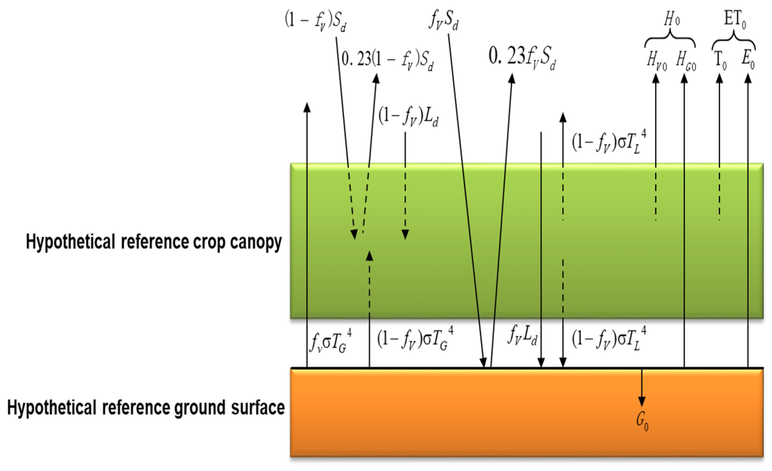
2.1. An Updated Reference-SPAC (R-SPAC) Model for ET₀

The present study updated the SPAC model developed by Wang and Yamanaka [28] to partition energy/water fluxes. Originally, the SPAC model were used to simulate the actual evapotranspiration (ET_a) and partition ET_a into transpiration (T) and evaporation (E). The existing SPAC model achieved good performance in partitioning ET in the humid grasslands of Japan [28], arid and semiarid grassland in Inner Mongolia [21], the typical ecosystem of the Heihe River Basin [25], and Alpine Meadow in Tibetan Plateau [29]. Therefore, we used the main equations of the SPAC model [28] and applied it on the reference land surface in this study. Figure 1 shows the modeling scheme adopted in the present study. Equation (1) and Equation (2) show the calculations for the balance between energy and radiation in the reference canopy of the plants and at the surface of the ground, respectively:

$$R_{nV}=(1-f_V)[0.77S_d+L_d+\sigma T_G{}^4-2\sigma T_L{}^4]=H_{V0}+l{T}_0$$

(1)

$$R_{nG}=f_V[0.77S_d+L_d]+(1-f_V)\sigma T_L{}^4-\sigma T_G{}^4=G_0+H_{G0}+l{E}_0$$

(2)

where R_nV represents the net radiation of the canopy of the reference plants (W m⁻²), T₀ represents the reference transpiration flux (kg m⁻² s⁻¹), H_V0 represents the sensible flux of heat from the canopy of the reference plants (W m⁻²), S_d is the short-wave radiation in a downward direction (W m⁻²), f_V denotes the permittivity of the canopy of plants, L_d is the long-wave radiation in a downward direction (W m⁻²), σ is 5.67 × 10⁻⁸ W m⁻² K⁻⁴ representing the Stefan–Boltzmann constant, T_G represents the temperature of the surface of the ground (°C), R_nG represents the surface of the ground net radiation (W m⁻²), T_L represents the temperature of leaves (°C), G₀ represents the heat flux of the ground (W m⁻²), H_G0 represents the flux of sensible heat of the surface of the ground (W m^–2), and E₀ represents the flux of evaporation (kg m⁻² s⁻¹). The reference crop per unit of area total flux is derived by adding those of the canopy of the plants and surface of the ground:

R_n = R_nV + R_nG, H₀ = H_V0 + H_G0, and lET₀ = l (E₀ + T₀).

(3)

The value of f_V is derived as a function of LAI:

$$f_V=1-\tanh (c_{LAI}LAI)$$

(4)

where C_LAI represents a constant, which is taken to be unity. The reference surface albedo values in the current study are 0.23 for both the canopy of the plants and surface of the surface. The leaf area index (LAI) was assumed to be 1 (m² m⁻²).

The T₀ and E₀ can be derived by:

$$T_0={\rho }_a[q_{sat}(T_L)-q_a]/(r_{aV}+r_c)$$

(5)

$$E_0={\rho }_a[q_{sat}(T_G)-q_a]/(r_{aG}+r_{ss})$$

(6)

where q_sat (T_G) and q_sat (T_L) represent specific humidity values at saturation for the surface of the ground and leaf and temperature, respectively (kg kg⁻¹), q_a represents the humidity of the air (kg kg⁻¹), and r_c and r_ss are the reference canopy resistance due to plant stomata and the resistance of the surface soil values, respectively, with both having constant values (70 s m⁻¹).

Similarly, the H_V0 and H_G0 are given as:

$$H_{V0}=c_p{\rho }_a(T_L-T_a)/r_{aV}$$

(7)

$$H_{G0}=c_p{\rho }_a(T_G-T_a)/r_{aG}$$

(8)

where r_aV represents aerodynamic resistance for the reference canopy of the plants (s m⁻¹) and r_aG represents resistance to aerodynamics posed by the surface of the ground (s m⁻¹).

r_aV and r_aG are calculated as [30]:

$$r_{aV}=\ln \left(\frac{z_m-d_0}{z_{0mV}}\right)\ln \left(\frac{z_h-d_0}{z_{0hV}}\right)/k^{2}u$$

(9)

$$r_{aG}=\ln \left(\frac{z_m}{z_{0mG}}\right)\ln \left(\frac{z_h}{z_{0hV}}\right)/k^2$$

(10)

where Z_m is height from which measurements of the speed of wind were taken, which is regarded as 2 m in the current study, d₀ represents the zero-plane height of displacement (m) and is taken to equal 0.666 × Z_V in the current study, where Z_V represents reference plant height, which is equal to 1.2 m in the current study, z_0mV represents the roughness length controlling the transfer of momentum above the reference canopy of the plants (m), and it is taken to be 0.123 × Z_V in the current study, Z_h represents the height at which measurements of temperature and humidity were taken, and it is regarded as 2 m in the current study, z_0hV is the length of roughness controlling the transfer of heat and vapor above the reference canopy of the plants (m), and it is taken to be 0.1 × z_0mV in the current study, k represents the von Karman’s constant, which is regarded to be 0.41 in the current study, u represents the speed of wind (m s⁻¹), z_0mG represents the length of roughness controlling the transfer of momentum above the surface of the ground (m), and it is regarded to be 10⁻⁴ in the current study, and z_0hG represents the length of roughness controlling the transfer of vapor and heat vapor above the surface of the ground (m), and it is taken to be 0.1 × z_0mG in the current study.

G₀ is calculated using the heat conduction law of Fourier as:

$$G_0={\lambda }_{soil}(T_G-T_{ss})/z_{soil}$$

(11)

where λ_soil represents the conductivity of heat at the soil surface (W m⁻¹ K⁻¹) and T_ss represents the temperature of the soil surface (°C) at depth Z_soil (m). λ_soil is assumed to be constant at 0.4 in the present study for the sake of simplicity, as it shows less sensitivity to variations in soil moisture in well-watered agricultural catchments.

2.2. Numerical Solution for ET₀ by the R-SPAC Model

The Newton-Raphson (NR) scheme can be used as a robust method of obtaining a solution with an improved convergence rate [31], and it has seen application for diagnostically resolving energy balance equations [32]. Introduction of the NR iteration scheme aimed to solve Equations (1) and (2) simultaneously for T_L and T_G, respectively. The provision of observed values of L_d, u, S_d, T_a, P, h_a, and T_soil allows the values of T_L and T_G to be derived for the calculation of all energy/water fluxes.

By rearranging Equations (1) and (2) with x equal to T_L and y equal to T_G, the following can be derived:

$$F(x,y)=(1-f_V)[0.77S_d+L_d+\sigma y^4]-2(1-f_V)\sigma x^4-c_p{\rho }_a(x-T_a)/r_{aV}-l{\rho }_a\left[q_{sat}(x)-q_a\right]/(r_{aV}+70)$$

(12)

$$G(x,y)=f_V[0.77S_d+L_d]+(1-f_V)\sigma x^4-\lambda (y-T_{ss})/z_{soil}-\sigma y^4-c_p{\rho }_a(y-T_a)/r_{aG}-l{\rho }_a\left[q_{sat}(y)-q_a\right]/(r_{aG}+70).$$

(13)

Close solutions of y and x that are more similar to actual values can be derived by iteratively solving the equation below:

$$\left(\begin{array}{c}\Delta x\\ \Delta y\end{array}\right)={\left(\begin{array}{cc}a& b\\ c& d\end{array}\right)}^{-1}\left(\begin{array}{c}-F\\ -G\end{array}\right)$$

(14)

$$a=\partial F/\partial x=-8(1-f_V)\sigma x_i{}^3-c_p{\rho }_a/r_{aV}-l{\rho }_a\frac{0.622}{P}\frac{l}{R_w{(x_i+273.16)}^2}{e}_{sat}(x_i)/(r_{aV}+70)$$

(15)

$$b=\partial F/\partial y=4(1-f_V)\sigma y_i{}^3$$

(16)

$$c=\partial G/\partial x=4(1-f_V)\sigma x_i{}^3$$

(17)

$$d=\partial G/\partial y=-4\sigma y_i{}^3-\lambda /z_{soil}-c_p{\rho }_a/r_{aG}-l{\rho }_a\frac{0.622}{P}\frac{l}{R_w{(y_i+273.16)}^2}{e}_{sat}(y_i)/(r_{aG}+70)$$

(18)

where Δx equals x_i+1 − x_i and Δy equals y_i+1 − y_i, in which i represents the iteration number, R_w represents the water vapor gas constant, and e_sat(x_i) or e_sat(y_i) are the vapor pressures at saturation at temperatures x_i or y_i, respectively. Iterations are halted when absolute values of Δy and Δx are below 0.0001.

Equations (12) and (13) exclude a correction in the stability of the atmosphere to avoid the procedure used in the iteration from becoming increasingly complicated. Thankfully, since the model excludes the use of known values of T_G and T_L, the calculated flux values are likely to have a lower sensitivity to the stability of the atmosphere, whereas calculated temperature values may show some affect.

2.3. The FAO-PM Model for Estimating ET₀

The FAO-PM method has proposed to be the accepted approach for determining ET₀ [1], and it is also used in the present study (Equation (19)):

$${\mathrm{ET}}_0=\frac{0.408\Delta ({\mathrm{R}}_n-\mathrm{G})+\gamma \frac{900}{T_a+273}{U}_2(e_s-e_a)}{\Delta +\gamma (1+0.34U_2)}$$

(19)

where R_n represents crop surface net radiation (MJ m⁻² day⁻¹), G represents the density of the flux of soil heat (MJ m⁻² day⁻¹), T_a represents the mean daily temperature of air at a 2 m height (°C), U₂ represents wind speed at a height of 2 m, e_s represents pressure of vapor at saturation (kPa), e_a is actual pressure of vapor (kPa), e_s − e_a represents the deficit in the vapor pressure at saturation (kPa), Δ is the pressure curve of slope vapor (kPa °C⁻¹), and γ represents the psychometric constant (kPa °C⁻¹).

2.4. An Analysis of the Sensitivity of the R-SPAC Model

The present study conducted a sensitivity analysis to better understand the relationship between variations in simulations of ET₀ by the R-SPAC and variations in model input factors using the method proposed by Wang and Yamanaka [28]. The sensitivity coefficient (S_i) can be determined as:

$$S_i=\frac{\partial O}{\partial p_i}\frac{p_i}{O}.$$

(20)

2.5. Model Validation Dataset

An actual meteorological and flux dataset were applied to the R-SPAC model, and simulations of ET₀ and actual ET_a were validated against that by the FAO-PM method and measurements by eddy covariance. These meteorological and flux datasets were obtained for Daman sites (38° 51′ N, 100° 22′ E, 1550 m) in an arid cropland of spring maize and artificial oasis in the mid reaches of the Heihe River Catchment, Zhangye, China, which forms a part of the Heihe Watershed Allied Telemetry Experimental Research (HiWATER) program [33]. The study site has a mean annual air temperature and precipitation of approximately 7.4 °C and 128.7 mm, respectively from 1961 to 2010, and a mean annual pan evaporation of 2002.5 mm. A field with an area about 13 ha around the site is used to plant maize only. Micrometeorological variables, including temperature of the air, relative humidity, speed of wind, four-component radiation, the profile of the temperature of the soil, and the flux of soil heat were recorded at 0.5 Hz, with means taken every 10 min using a collection of micrometeorological sensors installed above the plant canopy and in the soil. Data reported in the current study were averaged to hourly intervals from the 25th of May to the 15 September 2012 and used as input for modeling. Further details of data acquisition are described in the literature [34].

Simulated ET₀ partitioning results (e.g., T₀ and E₀) are difficult to be observed and determined in practice. Therefore, it is difficult to verify. However, associated actual evapotranspiration partitioning results (e.g., actual transpiration, T) can be observed in practice. In order to verify the model partitioning performance in the study site, we obtained the previous study of ET_a partitioning results estimated by the independent uWUE method [35].

3. Results

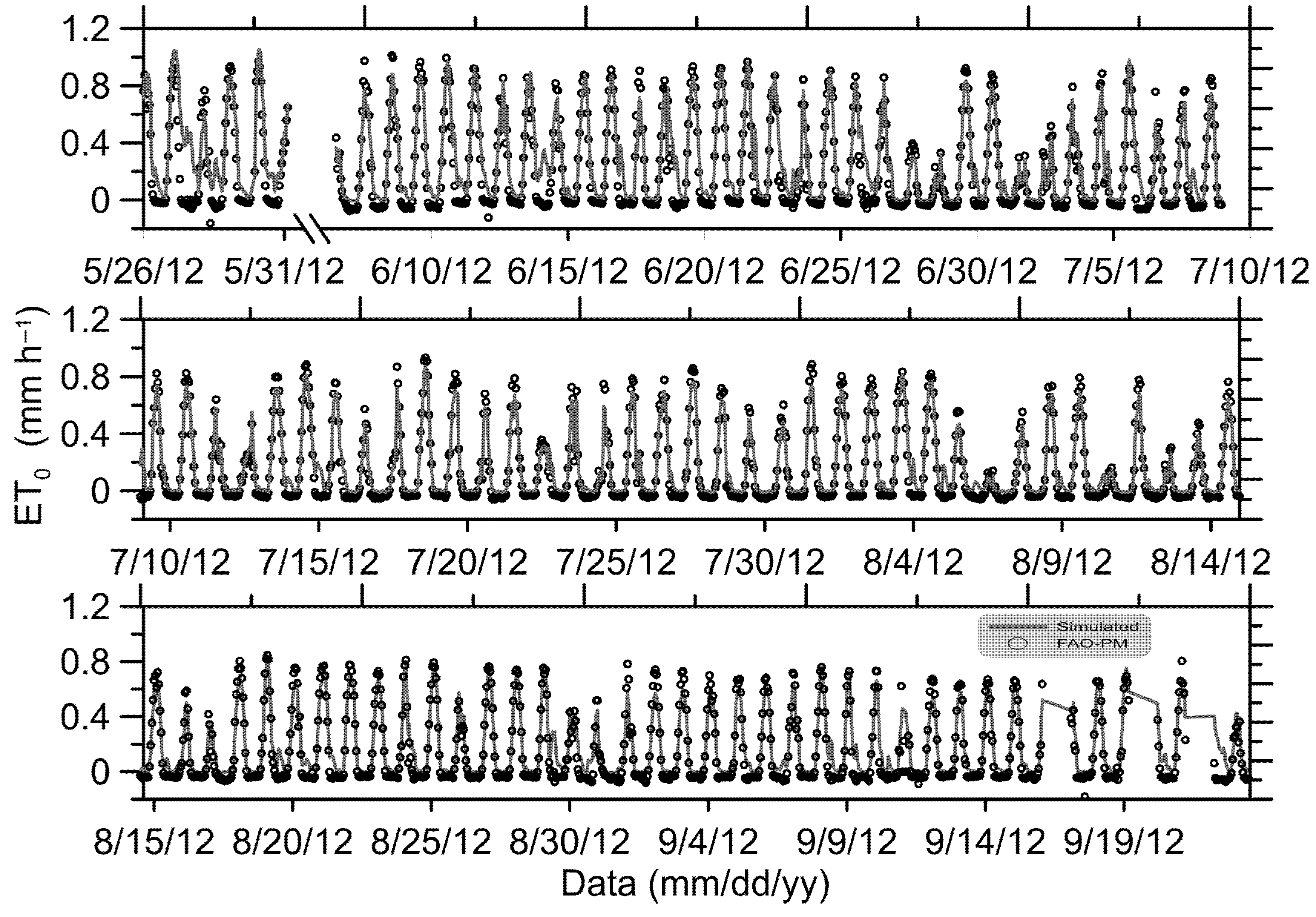
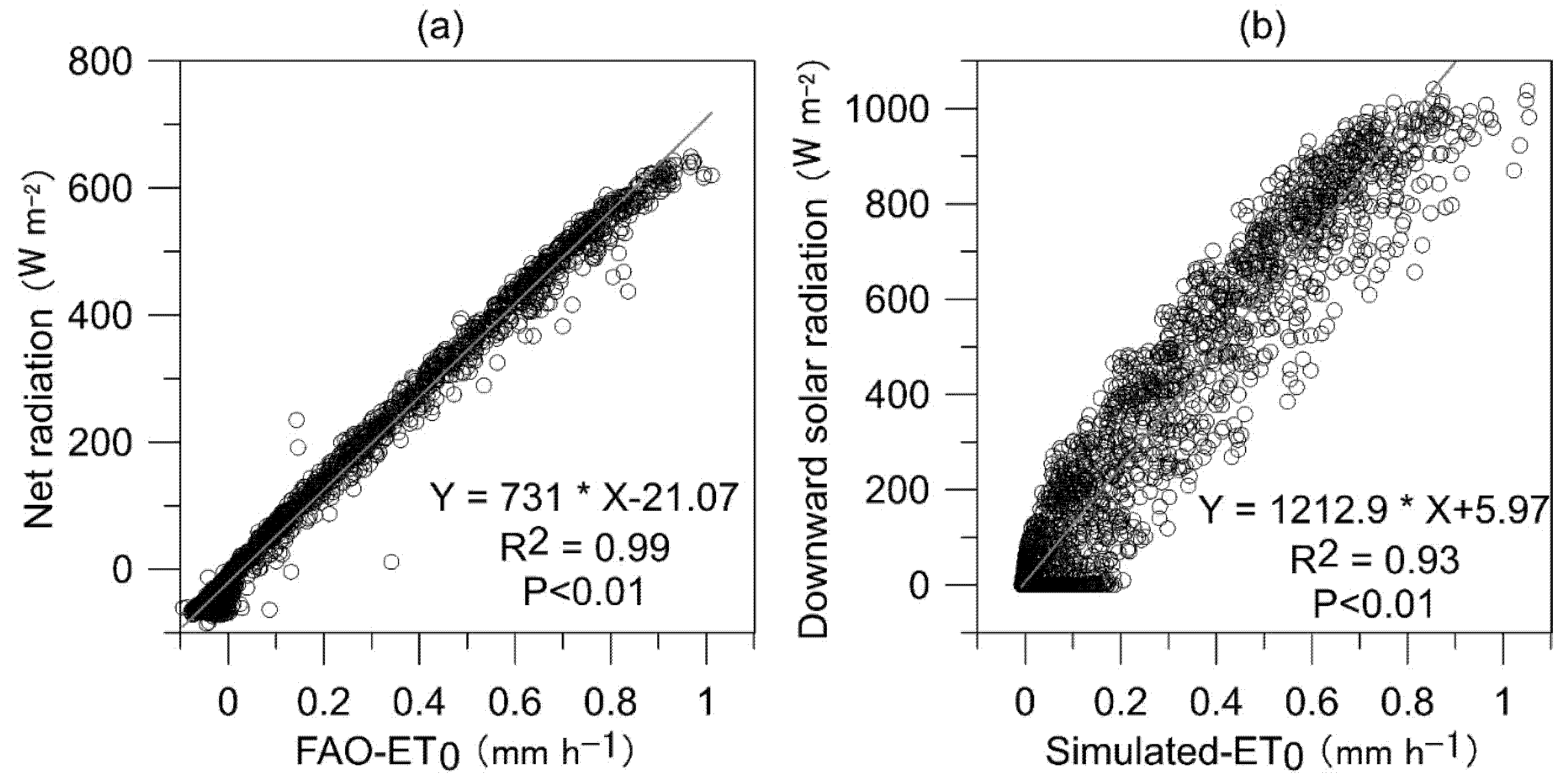
3.1. R-SPAC Model Performance in Simulating ET₀

The present study compared simulations of ET₀ between the FAO-PM and R-SPAC models (Figure 2). As shown in

Table 1. Statistical summary of the performance of the reference soil–plant–atmosphere continuum (R-SPAC) model in simulating reference evapotranspiration (ET₀) and associated SPAC in simulating actual evapotranspiration (ET_a) and its partitioning for actual transpiration (T).

Variables	Dataset	Unit	2 RMSD	I index	R2	n
Reference Evapotranspiration, ET0	All dataset	mm h−1	0.05	0.98	0.96	2813
	1 Daily time	mm h−1	0.05	0.99	0.96	1046
Actual Evapotranspiration, ETa	All dataset	W m−2	47.90	0.96	0.87	1464
3 Actual Transpiration, T	All dataset	mm h−1	0.11	0.82	0.80	335
	1 8:00am–16:00pm. 2 root mean square difference. 3 Hourly mean T dataset was obtained from Zhou et al., 2018 [35].

, the R-SPAC model simulations of ET₀ were similar to those of the FAO-PM model, as indicated by the index of agreement (I) of 0.99 and root-mean-square deviation (RMSD) of 0.05 mm h⁻¹. The simulations both of daily and diurnal variations by R-SPAC models were similar to those of estimated by FAO-PM, with an R² of 0.98.

In order to further demonstrate our modeling performance and its validity, we evaluate the modeling performance under the actual land surface conditions. For actual evapotranspiration (ET_a) and its partitioning (e.g., actual transpiration, T), as summarized in Table 1, the simulations of ET_a (T) have good agreement to measured ET_a (T) by eddy covariance (uWUE approach), as indicated by the index of agreement (I) of 0.96 (0.82) and RMSD of 47.90 W m⁻² (0.11 mm h⁻¹). The simulations of seasonal variations by the actual SPAC model were in agreement with those measured by EC and estimated by uWUE with an R² of 0.87 (0.80).

3.2. Seasonal Variations in ETo

Figure 3 shows the diurnal and seasonal variations in simulated ET₀ during the growing season by both the FAO-PM and R-SPAC models. The estimated means and seasonal variations in ET₀ by the FAO-PM and R-SPAC models were 0.18 mm h⁻¹ ± 0.29 mm h⁻¹ and 0.19 mm h⁻¹ ± 0.25 mm h⁻¹, respectively. Simulations of both models showed well-constructed diurnal and seasonal variations and no significant systematic bias (P < 0.01) during the growing season.

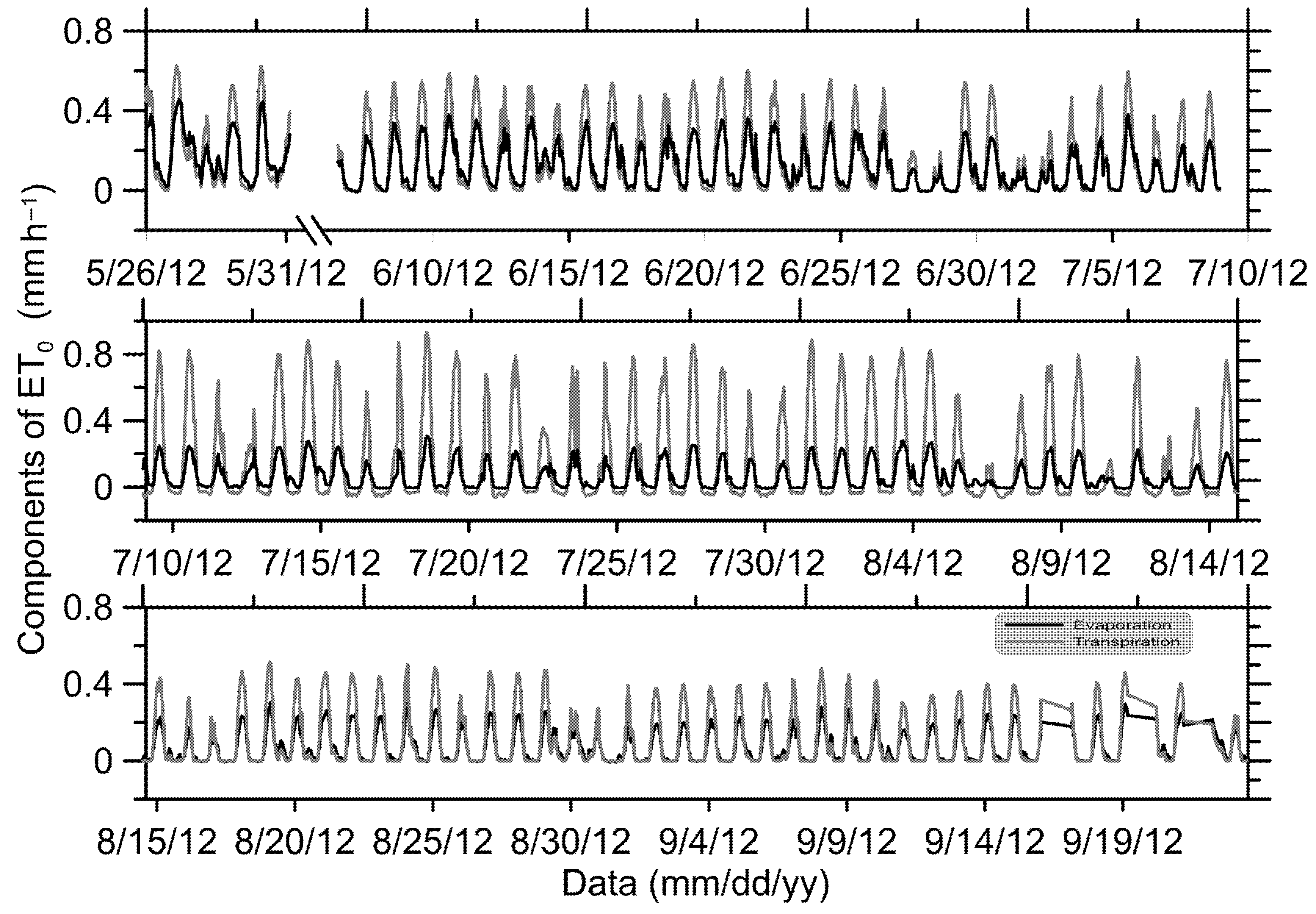
3.3. Partitioning of ET₀

Figure 4 illustrates diurnal and seasonal variations in simulated ET₀ components over the growing season by the R-SPAC model. The estimated mean and seasonal variation in ET₀ for soil evaporation (E₀) and plant transpiration (T₀) were 0.12 mm h⁻¹ ± 0.16 mm h⁻¹ and 0.09 mm h⁻¹ ± 0.09 mm h⁻¹, respectively. Dominant components of ET₀ at the study site are T₀ over the growing season, with the mean contribution and seasonal deviation of transpiration fraction (T₀/ET₀) being 0.63 ± 0.28.

3.4. Results of Sensitivity Analysis

Table 2. Mean and standard deviation in sensitivity coefficient (S_i) of reference evapotranspiration (ET₀) and its components (T₀ and E₀) to the measured variables.

Variables	Mean (s.d.)
	T0	E0	ET0
Sd	0.98 (0.30)	0.64 (0.23)	0.89 (0.29)
Ld	0.80 (0.47)	0.49 (0.31)	0.67 (0.39)
u	0.22 (0.14)	0.27 (0.11)	0.25 (0.12)
Ta	0.56 (0.13)	0.28 (0.25)	0.44 (0.13)
ha	−0.12 (0.20)	−0.42 (0.35)	−0.23 (0.25)
P	0.08 (0.11)	0.00 (0.10)	0.05 (0.10)
Tss	0.05 (0.06)	0.38 (0.24)	0.18 (0.15)

s.d., standard deviation; S_d, downward short-wave radiation; L_d, downward long-wave radiation; u, wind speed; T_a, air temperature; h_a relative humidity; P, air pressure; T_ss, soil surface temperature at depth Z_ss.

shows the sensitivity of input variables to ET₀ and its components. Among many climate factors, downward short-wave radiation (S_d) was the most sensitive to ET₀, followed by downward long-wave radiation (L_d) and air temperature (T_a). Changes in S_d, L_d and T_a of 5% resulted in changes in ET₀ of 4.4%, 3.3%, and 2.2% respectively. For T₀, S_d was the most sensitive factors with sensitivity coefficient of 0.98; L_d and T_a followed with sensitivity coefficients 0.80 and 0.56. For E₀, S_d was the most sensitive factor followed by L_d and relative humidity (h_a). Changes in S_d, L_d, and h_a of 5% resulted in changes in E₀ of 3.2%, 2.4%, and −2.1%, respectively.

4. Discussion

4.1. Modeling Advantages and Limitations

The updated R-SPAC model proposed in the present study showed a good performance in simulating ET₀ when compared against the FAO-PM approach. These results of the present study confirmed the validity and usefulness of the use of the R-SPAC model for estimating ET₀ in a reference agricultural catchment. Although previous studies have shown similar performances to that of the current study through the use of other approaches [8,9,19,36,37], the use of the R-SPAC model offers various advantages. Firstly, the approach proposed in the present study allows the consideration and parameterization of plant factors that affect ET, including crop type, continuous growth processes characterized by leaf area index and canopy height development, and crop canopy structure that affects the plant canopy and geometry. Secondly, the R-SPAC model provides a rigorous consideration of the balance between energy and radiation in both the canopy of reference plants and at the surface of the ground, as well as their interactions, thereby facilitating the estimation of all the components of the energy balance. These estimations can then be validated against those of the standard FAO-PM model. Thirdly, the R-SPAC uses the NR scheme to estimate T_L and T_G in a simple, stable, and rapid manner without the need for measurements of directional radiometric temperature; meanwhile, the estimations of T_L and T_G are more sensitive to the partitioning of ET compared to ET itself, and they can be useful for the validation of models. Based on the calculated T_L and T_G, the partitioning of ET becomes a matter of course. However, there remains scope for further modification and improvement of the R-SPAC model. The present study used arbitrarily constant values for some parameters (e.g., LAI, Z_V, and albedo of 1 m² m⁻², 1.2 m, and 0.23, respectively) throughout the periods investigated, and these assumptions may account for errors in estimating crop-specific ET_C. The present study focus on ET₀ without considering various management practices (e.g., Plastic mulches) and not consider dynamics in the non-growing season [20,25].

4.2. Controls of ET₀

Increasing attention to global warming has produced many reports on decreasing trends in reference evapotranspiration and the associated climatic controls. These trends are likely the result of decreases in sunshine duration over China [38] that may be related to increases in air pollution and atmospheric aerosols [39], increases in cloud cover [40], and decreased wind speed [41]. A study in the Jinhe River Basin showed that reductions in ET₀ were principally the result of significant decreases in wind speed as well as sunshine hours [42]. The present study identified perhaps net radiation (Figure 5a) or short-wave radiation (Figure 5b) as the main drivers of seasonal variations in ET₀ through changing available energy (R_n-G). Although some previous reports [41] have emphasized the importance of wind speed in driving variations in ET₀, the results of the present study suggest that variation in solar radiation is the dominant driver of ET₀, at least at the study site of the present study.

4.3. Implications and Prospective Research Directions

Evapotranspiration is a comprehensive result of the interaction of climate, vegetation, and soil, which can be esitimated by ET₀, ET_p, and ET_a, respectively [1,27,43]. A reference evapotranspiration (ET₀) and its components (reference transpiration and reference soil evaporation) are calculated assuming that the reference land surface is wet and well managed [1]. A potential evapotranspiration (ET_p) and its components (potential transpiration and potential soil evaporation) are calculated assuming that when the land surface is wet, total evapotranspiration flux consumes the whole available energy [27]. The ET_a and its components are calculated by actual land surface conditions [28,44]. The successful application of the R-SPAC model to the scheduling of irrigation (e.g., dynamics of the crop coefficient) requires determining the relationship between reference crop ET and ET of the target crop through the use of crop growth information (e.g., dynamics of leaf area index (LAI) and Z_V, stomatal behavior). The model shows promise for the calculation of the continuous crop coefficients (C_p = ET₀/ET_p) as well as ecosysytem/plant water stress coefficients (K_s = ET_a/ET_p) throughout the growing season under various land surface scenarios; for example, reference land surface for ET₀, actual land surface with adequate soil moisture for ET_p, and actual land surface with actual soil moisture for ET_a [25,28]. Moreover, the model can be further extended to esitimated ET₀, ET_p, and ET_a in non-agricultural ecosystems, such as forests and other perennial vegetation [27,43]. It is promising to quantify the seasonal dynamics of C_P and K_S in different ecosystems, which is of great significance for predicting the ecohydrological response to climate change and accurately quantifying the water use on basins to global scale.

5. Conclusions

The present study updated and applied the R-SPAC model for the simulation of diurnal and seasonal variations in ET₀. Simulations of ET₀ by the R-SPAC model were consistent with those of the FAO-PM model, thereby confirming the accuracy of the R-SPAC model. The present study used sensitivity analysis to explore uncertainties/errors in ET₀ and components in input variables. The results of the present study showed that the R-SPAC model is a useful tool to partition ET₀. The present study showed that the principal factor controlling diurnal and seasonal variations in ET₀ at the investigated site is solar radiation. It is promising to estimate ET₀, ET_p, and ET_a under various land surface scenarios and quantify the seasonal dynamics of C_P and K_S in crop and other different ecosystems.

References

1. Allen, R.G.; Pereira, L.S.; Raes, D.; Smith, M. Crop Evapotranspiration: Guidelines for Computing Crop Water Requirements. FAO Irrigation and Drainage Paper No. 56; FAO: Rome, Italy, 1998. [Google Scholar]
2. Wang, T.; Melton, F.S.; Pas, I.; Johnson, L.F.; Thao, T.; Post, K.; Florence, C.S. Evaluation of crop coefficient and evapotranspiration data for sugar beets from landsat surface reflectances using micrometeorological measurements and weighing lysimetry. Agric. Water Manag. 2021, 244, 106533. [Google Scholar] [CrossRef]
3. Semmens, K.A.; Anderson, M.C.; Kustas, W.P.; Gao, F.; Alfieri, J.G.; McKee, L.; Prueger, J.H.; Hain, C.R.; Cammalleri, C.; Yang, Y.; et al. Monitoring daily evapotranspiration over two California vineyards using Landsat 8 in a multi-sensor data fusion approach. Remote Sens. Environ. 2016, 185, 155–170. [Google Scholar] [CrossRef] [Green Version]
4. Turc, L. Estimation des besoins en eau d’irrigation, evapotranspiration potentielle, formule climatique simplifiee etmise a jour. Ann. Agron. 1961, 12, 13–49. [Google Scholar]
5. Monteith, J.L. Evaporation and Environment. Symp. Soc. Exp. Biol. 1965, 19, 205–234. [Google Scholar]
6. Burt, C.M.; Mutziger, A.J.; Allen, R.G.; Howell, T.A. Evaporation research: Review and interpretation. J. Irrig. Drain. Eng. 2005, 131, 37–58. [Google Scholar] [CrossRef] [Green Version]
7. Guan, H.; Wilson, J.L. A hybrid dual-source model for potential evaporation and transpiration partitioning. J. Hydrol. 2009, 377, 405–416. [Google Scholar] [CrossRef]
8. McVicar, T.R.; Van Niel, T.G.; Li, L.-T.; Hutchinson, M.F.; Mu, X.-M.; Liu, Z.-H. Spatially distributing monthly reference evapotranspiration and pan evaporation considering topographic influences. J. Hydrol. 2007, 338, 196–220. [Google Scholar] [CrossRef]
9. Pˆoças, I.; Calera, A.; Campos, I.; Cunha, M. Remote sensing for estimating and mapping single and basal crop coefficientes: A review on spectral vegetation indices approaches. Agric. Water Manag. 2020, 233, 106081. [Google Scholar] [CrossRef]
10. Pereira, L.; Paredes, P.; Melton, F.; Johnson, L.; Wang, T.; L’opez-Urrea, R.; Cancela, J.; Allen, R. Prediction of crop coefficients from fraction of ground cover and height. Background and validation using ground and remote sensing data. Agric. Water Manag. 2020, 241, 106197. [Google Scholar] [CrossRef]
11. Pôças, I.; Paço, T.A.; Paredes, P.; Cunha, M.; Pereira, L.S. Estimation of actual crop coefficients using remotely sensed vegetation indices and soil water balance modelled data. Remote Sens. 2015, 7, 2373–2400. [Google Scholar] [CrossRef] [Green Version]
12. Harbeck, E. A practical and field technique for measuring reservoir evaporation utilizing mass-transfer theory. Geol. Surv. Prof. Pap. Wash. 1962, 272, 100–105. [Google Scholar]
13. Mohammad, J.; Hamidreza, K.; Ali, K.; Akbar, M. Estimation of evapotranspiration and crop coefficient of drip-irrigated orange trees under a semi-arid climate. Agric. Water Manag. 2021, 248, 106769. [Google Scholar] [CrossRef]
14. Thornthwaite, C.W. An Approach toward a Rational Classification of Climate: The Geographical Review; Taylor & Francis Ltd.: New York, NY, USA, 1948; Volume 38, pp. 55–94. [Google Scholar]
15. Xu, C.Y.; Singh, V.P. Evaluation and generalization of temperature-based methods for calculating evaporation. Hydrol. Process. 2001, 15, 305–319. [Google Scholar] [CrossRef] [Green Version]
16. Xu, C.Y.; Singh, V.P. Evaluation and generalization of radiation based methods for calculating evaporation. Hydrol. Process. 2000, 14, 339–349. [Google Scholar] [CrossRef]
17. Sumner, D.M.; Jacobs, J.M. Utility of Penman–Monteith, Priestley–Taylor, reference evapotranspiration, and pan evaporation methods to estimate pasture evapotranspiration. J. Hydrol. 2005, 308, 81–104. [Google Scholar] [CrossRef]
18. Shuttleworth, W.J.; Wallace, J.S. Evaporation from sparse crops—An energy combination theory. Q. J. R. Meteorol. Soc. 1985, 111, 839–855. [Google Scholar] [CrossRef]
19. Kustas, W.P.; Norman, J.M. A two-source approach for estimating turbulent fluxes using multiple angle thermal infrared observations. Water Resour. Res. 1997, 33, 1495–1508. [Google Scholar] [CrossRef]
20. Wang, P.; Deng, Y.J.; Li, X.Y.; Wei, Z.; Hu, X.; Tian, F.; Wu, X.; Huang, Y.; Ma, Y.J.; Zhang, C.; et al. Dynamical effects of plastic mulch on evapotranspiration partition in a mulched agriculture ecosystem: Measurement with numerical modeling. Agric. For. Meteorol. 2019, 268, 98–108. [Google Scholar] [CrossRef]
21. Wang, P.; Li, X.Y.; Wang, L.X.; Wu, X.C.; Hu, X.; Fan, Y.; Tong, Y.Q. Divergent evapotranspiration partition dynamics between shrubs and grasses in a shrub-encroached steppe ecosystem. New Phytol. 2018, 219, 1325–1337. [Google Scholar] [CrossRef] [PubMed] [Green Version]
22. Norman, J.M.; Anderson, M.C.; Kustas, W.P.; French, A.N.; Mecikalski, J.; Torn, R.; Diak, G.R.; Schmugge, T.J.; Tanner, B.C.W. Remote sensing of surface energy fluxes at 101-m pixel resolutions. Water Resour. Res. 2003, 39, 1221. [Google Scholar] [CrossRef] [Green Version]
23. Anderson, M.C.; Norman, J.M.; Mecikalski, J.R.; Torn, R.D.; Kustas, W.P.; Basara, J.B. A multiscale remote sensing model for disaggregating regional fluxes to micrometeorological scales. J. Hydrometeorol. 2004, 5, 343–363. [Google Scholar] [CrossRef]
24. Norman, J.M.; Becker, F. Terminology in thermal infrared remote sensing of natural surfaces. Agric. For. Meteorol. 1995, 77, 153–166. [Google Scholar] [CrossRef]
25. Tong, Y.; Wang, P.; Li, X.Y.; Wang, L.; Wu, X.; Shi, F.; Bai, Y.; Li, E.; Wang, J.; Wang, Y. Seasonality of the transpiration fraction and its controls across typical ecosystems within the Heihe River Basin. J. Geophys. Res. Atmos. 2019, 124, 1277–1291. [Google Scholar] [CrossRef] [Green Version]
26. Kustas, W.P.; Norman, J.M. A two-source energy balance approach using directional radiometric temperature observations for sparse canopy covered surfaces. Agron. J. 2000, 92, 847–854. [Google Scholar] [CrossRef]
27. Peng, L.; Zeng, Z.; Wei, Z.; Chen, A.; Wood, E.F.; Sheffield, J. Determinants of the ratio of actual to potential evapotranspiration. Glob. Chang. Biol. 2019, 25, 1326–1343. [Google Scholar] [CrossRef] [Green Version]
28. Wang, P.; Yamanaka, T. Application of a two-source model for partitioning evapotranspiration and assessing its controls in temperate grasslands in central Japan. Ecohydrology 2014, 7, 345–353. [Google Scholar] [CrossRef]
29. Cui, J.; Tian, L.; Wei, Z.; Huntingford, C.; Wang, P.; Cai, Z.; Ma, N.; Wang, L. Quantifying the controls on evapotranspiration partitioning in the highest alpine meadow ecosystem. Water Resour. Res. 2020, 55, 1–22. [Google Scholar] [CrossRef]
30. Brutsaert, W. Evaporation in the Atmosphere. Theory, History, and Applications; Reidel Dordrecht: Boston, MA, USA; London, UK, 1982. [Google Scholar]
31. Paniconi, C.; Putti, M. A comparison of Picard and Newton iteration in the numerical solution of multidimensional variably saturated flow problems. Water Resour. Res. 1994, 30, 3357–3374. [Google Scholar] [CrossRef]
32. Yamanaka, T.; Takeda, A.; Sugita, F. A modified surface-resistance approach for representing bare-soil evaporation: Wind-tunnel experiments under various atmospheric conditions. Water Resour. Res. 1997, 33, 2117–2128. [Google Scholar] [CrossRef]
33. Li, X.; Cheng, G.D.; Liu, S.M.; Xiao, Q.; Ma, M.G.; Jin, R.; Che, T.; Liu, Q.H.; Wang, W.Z.; Qi, Y.; et al. Heihe watershed allied telemetry experimental research (HiWATER): Scientific objectives and experimental design. Bull. Am. Meteorol. Soc. 2013, 571, 1145–1160. [Google Scholar] [CrossRef]
34. Liu, S.; Xu, Z.; Song, L.; Zhao, Q.; Ge, Y.; Xu, T. Upscaling evapotranspiration measurements from multi-site to the satellite pixel scale over heterogeneous land surfaces. Agric. For. Meteorol. 2016, 230, 97–113. [Google Scholar] [CrossRef]
35. Zhou, S.; Yu, B.; Zhang, Y.; Huang, Y.; Wang, G. Water use efficiency and evapotranspiration partitioning for three typical ecosystems in the Heihe river basin, northwestern china. Agric. For. Meteorol. 2018, 253, 261–273. [Google Scholar] [CrossRef]
36. Ahmed, E.; Jinsong, D.; Ke, W.; Anurag, M.; Saman, M. Modeling long-term dynamics of crop evapotranspiration using deep learning in a semi-arid environment. Agric. Water Manag. 2020, 241, 106334. [Google Scholar] [CrossRef]
37. Evett, S.R.; Schwartz, R.C.; Howell, T.A.; Louis Baumhardt, R.; Copeland, K.S. Can weighing lysimeter ET represent surrounding field ET well enough to test flux station measurements of daily and sub-daily ET? Adv. Water Resour. 2012, 50, 79–90. [Google Scholar] [CrossRef]
38. Kaiser, D.P.; Qian, Y. Decreasing trends in sunshine duration over China for 1954–1998: Indication of increased haze pollution? Geophys. Res. Lett. 2002, 29, 2042. [Google Scholar] [CrossRef]
39. Liepert, B.G.; Feichter, J.; Lohmann, U.; Roeckner, E. Can aerosols spin down the water cycle in a warmer and moister world? Geophys. Res. Lett. 2004, 31, L06207. [Google Scholar] [CrossRef] [Green Version]
40. Dai, A.; Tenberth, K.E.; Karl, T.R. Effects of clouds, soil moisture, precipitation and water vapor on diurnal Temperature range. J. Clim. 1999, 12, 2451–2473. [Google Scholar] [CrossRef]
41. Yin, Y.; Wu, S.; Chen, G.; Dai, E. Attribution analyses of potential evapotranspiration changes in China since the 1960s. Theor. Appl. Climatol. 2009, 101, 19–28. [Google Scholar] [CrossRef]
42. Wang, P.; Yamanaka, T.; Qiu, G.Y. Causes of decreased reference evapotranspiration and pan evaporation in the Jinghe River catchment, northern China. Environmentalist 2012, 32, 1–10. [Google Scholar] [CrossRef]
43. Liu, C.; Sun, G.; McNulty, S.G.; Noormets, A.; Fang, Y. Environmental controls on seasonal ecosystem evapotranspiration/potential evapotranspiration ratio as determined by the global eddy flux measurements. Hydrol. Earth Syst. Sci. 2017, 21, 311–322. [Google Scholar] [CrossRef] [Green Version]
44. Wei, Z.; Lee, X.; Wen, X.; Xiao, W. Evapotranspiration partitioning for three agro-ecosystems with contrasting moisture conditions: A comparison of an isotope method and a two-source model calculation. Agric. For. Meteorol. 2018, 252, 296–310. [Google Scholar] [CrossRef]
Figure 1. An updated reference: soil-plant-atmosphere continuum (R-SPAC) model for estimating reference evapotranspiration and its components, updated from Wang and Yamanaka, 2014 [28]. All symbols used are defined in the text.
Agriculture 11 00385 g001
Figure 2. Similarity of simulations of reference evapotranspiration (ET0) by the Penman–Monteith approach by the Food and Agriculture Organization (FAO-PM) and the reference soil–plant–atmosphere continuum (R-SPAC) model.
Agriculture 11 00385 g002
Figure 3. Seasonal variations in simulated reference evapotranspiration (ET0) by two models during the growing season. The gray lines represent simulations by the reference soil-plant-atmosphere continuum (R-SPAC) model, whereas black dots represent simulations by the Penman–Monteith model by the Food and Agriculture Organization (FAO-PM).
Agriculture 11 00385 g003
Figure 4. Seasonal variations in reference evapotranspiration (ET0) components as simulated by the reference soil–plant–atmosphere continuum (R-SPAC) model over the growing season. The gray line represents shows transpiration, whereas the black line represents reference evaporation.
Agriculture 11 00385 g004
Figure 5. Relationship between downward solar radiation and reference evapotranspiration (ET0) simulated by (a) the Penman–Monteith method by the Food and Agriculture Organization (FAO-PM) and (b) the reference soil–plant–atmosphere continuum (R-SPAC) model.
Agriculture 11 00385 g005