Travel Reduction Control of Distributed Drive Electric Agricultural Vehicles Based on Multi-Information Fusion

Abstract

In agricultural vehicles with internal combustion engines, owing to the use of rear-wheel drive or four-wheel drive, it is difficult to obtain information regarding the slip of the driving wheels. Excessive wheel slip, an inevitable phenomenon occurring during agricultural activities, can easily damage the original soil surface and result in excessive energy consumption. To solve these problems, a distributed drive agricultural vehicle (DDAV) based on multi-information fusion was proposed. The actual travel reduction of each wheel was calculated by determining the vehicle parameters in order to deliver the required torque to the four drive wheels via sliding mode control (SMC) and incremental proportional-integral (PI) control. Through this process, the vehicle always operates in a straight line. Test results show that, on a uniform surface, the travel reduction of each wheel can be maintained at the target value by using the incremental PI control strategy, with only minor fluctuations, to make the vehicle run in a straight line (R² = 0.9999). Furthermore, on a separated surface, the travel reduction of each wheel can be maintained at the target value, and using the SMC strategy enables more identical coefficient of gross tractions for each wheel to make the vehicle run in a straight line (R² = 0.9902). Unlike the non-control strategy, the vehicle reaches a stable state within 1 s, owing to the use of a controller that can effectively reduce the impact of road changes on vehicle velocity. This study can provide a reference for the drive control of DDAVs.

1. Introduction

The field operation of wheeled agricultural vehicles is an important part of agricultural production. To realize precise and intelligent agriculture, one approach is to ensure that these vehicles precisely perceive and identify their working state and environment through sensors. Recently, owing to the rapid increase in research on distributed drive agricultural vehicles [1,2,3], especially agricultural vehicles driven by servo motors, these vehicles can also be equipped with inertial navigation, GPS, cameras, and other sensors. Through multi sensor information fusion, more intelligent and accurate vehicles featuring improved driving control or power consumption control can be achieved. Multi sensor information fusion is an information processing method that can improve the detection performance of the system, expand the space-time coverage, improve the reliability and maintainability of the system, and improve fault tolerance and robustness. It is widely used in intelligent vehicle driving, agricultural robots, agricultural machinery navigation, unmanned farms, and other such fields. Rear-wheel drive and four-wheel drive are the most common forms of power transmission employed in agricultural vehicles with internal combustion engines; however, in these configurations, the driving force of each driving wheel, subjected to the differential, cannot be controlled independently. In contrast, in distributed drive agricultural vehicles, power is transmitted directly to the drive wheels or driving motors are installed near the wheels, which shortens the drive chain and significantly improves the transmission efficiency. In addition, the drive motor itself serves as an information unit that can accurately provide feedback regarding the current wheel speed and driving torque. This enables fast and accurate control [4], in addition to high reliability and good flexibility [5], providing a suitable foundation for multi-information fusion in vehicles.

During the operation of agricultural vehicles with internal combustion engines, owing to the complex soil environment and the large load fluctuations, it is difficult to obtain accurate information regarding the operation and traction state of the vehicle. When the travel reduction of the driving wheel exceeds 0.2, excessive driving wheel slip occurs; as a result, the traction force of the vehicle is limited, and the growth environment of the crops can be damaged. Thus, the travel reduction directly affects the dynamic performance of an agricultural vehicle, and it is an important parameter for real-time control systems [6,7]. It is necessary to maintain the travel reduction of each driving wheel within the allowable range to improve the traction efficiency of agricultural vehicles.

In the case of electric drive vehicles, the driving, anti-skid mechanism, and tracking are generally realized by a motor control strategy [8], such as the model predictive control [9,10], hierarchical control strategy [11], or electronic stability control algorithm [12]. Sliding mode control (SMC) is a variable structure control method [13] that has been widely used in mechanical and vehicle engineering [14,15], especially for clutch control [16] and motor control [17]. Although some studies have focused on the control of agricultural vehicles in terms of the path [18] and guidance and steering [19], the drive control of distributed drive agricultural vehicles on complex soil surfaces has received limited attention. Furthermore, the agricultural environment and soil conditions of each wheel can be complex and considerably different. Therefore, each wheel requires a separate travel reduction control to ensure that a reasonable amount of torque is delivered to the wheel.

This study introduces a distributed operation platform driven by servo motors and controlled by programmable logic controller (PLC) and configuration software to address the abovementioned problems related to the driving and control of distributed drive agricultural vehicles on complex soil surfaces. Multi-information fusion, based on the vehicle GPS and servo driver, was applied for monitoring the travel reduction of each wheel, and a vehicle body controller based on sliding film control and incremental proportional-integral (PI) control was designed to realize the driving of vehicles on different soil surfaces. Uniform and separated surfaces experiments were selected to test performance of the strategies, compared with non-control strategies. The proposed approach was expected to effectively reduce wheel slip and improve the traction efficiency of distributed drive agricultural vehicles, while also ensuring traction stability.

2. Materials and Methods

The experimental electric agricultural vehicle developed in this study utilizes four-wheel independent drive and rear-wheel steering (Figure 1), and the main parameters are shown in

Table 1. Main parameters of the experimental DDAV.

Parameters	Value
Power	18 KW
Vehicle size	3.2 m × 2.0 m × 2.7 m
Trackwidth	1.6–2.8 m
Wheelbase	2.2 m
Vehicle mass	2000 kg
Max mass	3000 kg
Tire	8.3–24
Centroid coordinate	(1.12, 0, 1.763) m

.

The control system is mainly composed of the controller, actuators, and information collectors. The vehicle drive controller continuously receives and processes signals collected by the sensors, and calculates the travel reduction of each driving wheel based on the current vehicle speed and wheel speed. In this strategy, each actuator is assigned different instructions to complete the command action according to the final signal processing results. Moreover, the servo driver feeds back the executed signal to the controller to complete the closed-loop control.

Siemens PLC S7-200 was chosen as the controller; it mainly includes a central processing unit (CPU) module (EM214), an analog input module (EM231, sampling frequency 200 Hz), and an analog output module (EM232, output frequency 500 Hz). It is capable of high-speed signal acquisition, torque signal acquisition, and basic I/O functions, adequate for the tests in this study. Monitor and control generated system (MCGS), developed by Beijing Kunlun TongTai Automation Software Technology Co., Ltd. Beijing, China, was selected as the configuration software. It can realize field data acquisition and monitoring, and also process and control front-end data. In this study, MCGS was mainly used as the platform for data storage and foreground observation; it can quickly exchange memory values with the PLC, display the required value in the form of a chart, and subsequently save it as a database file.

The wheels were directly driven by servo motors and reducers, that, in turn, were controlled by the torque mode. The Panasonic A52 series MFME454G1G flat servo motor was selected as the drive motor. The matching drive model was MFDTB3A2, and appearance identification was F type. GPS was adopted for speed measurement; the GNSS differential receiver system, produced by JAVAD (accuracy of RTK, 0.8 cm + 1 ppm; accuracy of velocity, 0.02 m/s), was mainly divided into the base station and the mobile station. The mobile station features primary and secondary antennas that can detect the vehicle’s heading angle and global coordinate position. The structure of hardware device is shown as Figure 2.

Generally, the barycenter rolling and vehicle laterally slipping are inevitable when agricultural vehicles are steering. However, most of them are under the conditions of turning around and obstacle avoidance in the field. This article mainly discusses the sliding of agricultural vehicles under the conditions of field operation, such as ploughing, sowing, and fertilization. Therefore, to establish a dynamic model of the vehicle, two assumptions were made in this study: the geometric parameters of all wheels were assumed to be identical, and the vehicle was assumed to move along a straight path.

The traction force of each wheel can be adjusted according to the specific driving state of the vehicle. The wheels on the same side can be regarded as a two-wheel vehicle model, as shown in Figure 3, and subscript 1, 2, 3, and 4 indicates left front, left rear, right front, and right rear, respectively.

Hence, the vehicle dynamic model can be expressed as:

$$m\dot{v}={{\displaystyle \sum }}_{i=1}^4{F}_{xi}-{{\displaystyle \sum }}_{i=1}^4{X}_i(i=1,2,3,4)$$

(1)

The equation of torque balance of the driving wheel can be shown as:

$$J{\dot{\omega }}_i=T_{di}-F_{xi}r-F_{zi}fr$$

(2)

where r = tire rolling radius, ω = angular velocity of the wheels, J = rotational moment of inertia of the wheels, m = mass of the vehicle,$T_d$ = input torque of drive wheel,$F_x$ = longitude force of drive wheel$, F_z$ = normal force of drive wheel, f = rolling friction coefficient of wheels, and X = running resistance of wheel.

$$F_{i,trac}=F_{xi}-X_i(i=1,2,3,4)$$

(3)

$$F_{res}=F_{xi}r+F_{zi}fr$$

(4)

Then, based on Equations (6)–(8), the dynamic equations can be shown as follows:

$$m\dot{v}={{\displaystyle \sum }}_{i=1}^4{F}_{i,trac}$$

(5)

$$J{\dot{\omega }}_i=T_{di}-F_{res}$$

(6)

The coefficient of gross traction ${\mu }_i$ can be defined as:

$${\mu }_i=\frac{F_{xi}}{F_{zi}}\approx \frac{T_{fd}}{F_{zi}}$$

(7)

where$T_{fd}$ = the feedback torque of wheel obtained by servo motor.

For traditional machinery, when one wheel is completely slipping, the driving force of the other wheel is also greatly reduced because of the differential. Although it can ensure that the vehicle runs in a straight line, it reduces the overall efficiency. The power units on each wheel (a remarkable feature of distributed electric drive agricultural vehicles) can be controlled independently to adjust the driving force according to the change of the road surface to ensure the driving stability of agricultural vehicles. For traditional agricultural vehicles, inappropriate driving is one of the prime reasons that driving cannot follow the driving intention. Instead of increasing the adhesion or stopping to solve the invalid-driving problem, the distributed drive agricultural vehicle can change its driving state by controlling the independent motors.

The travel reduction of four driving wheels is defined as:

$$s_i=\frac{r{\omega }_i-v}{r{\omega }_i}, (i=1,2,3,4)$$

(8)

where$s_i$ = travel reduction of the vehicle, ${\omega }_i$ = the angular velocity of the wheels, v = vehicle velocity, and r = tire rolling radius.

Speed measurement is the key to calculating the travel reduction. Different methods are suitable for different situations. In the field environment, GPS is more suitable for measuring vehicle speed than other methods [20]. Therefore, this study used GPS to measure vehicle speed.

2.1. Drive Control Based on SMC

At present, soil parameters are mainly predicted according to existing research parameters or are estimated by experimental methods. The SMC can effectively solve the problem of nonlinear systems with uncertain parameters. Therefore, in this study, SMC was used to control the driving torque.

The state equation of the control system was constructed, and a system equation can be as follows, which is calculated by Equations (5) and (6) and derivative of Equation (8).

$$\dot{s_i}=\frac{r{(1-s_i)}^2\left(T_{di}-T_{i,res}\right)}{Jv}-\frac{\left(1-s_i\right){{\displaystyle \sum }}_{i=1}^4{F}_{i,trac}}{Mv}(i=1,2,3,4)$$

(9)

Equation (8) can be transferred to:

$$\dot{\mathit{s}}=\mathit{h}\left(\mathit{s},v\right)+\mathit{g}\left(\mathit{s},v\right)\mathit{u}$$

(10)

$$\mathit{s}={[s_1{s}_2{s}_3{s}_4]}^{\mathrm{T}}$$

(11)

$$\mathit{u}={[T_{d1} T_{d2} T_{d3} T_{d4}]}^{\mathrm{T}}$$

(12)

$$\mathit{h}\left(\mathit{s},v\right)={[h_1\left(s,v\right)h_2\left(s,v\right)h_3\left(s,v\right)h_4\left(s,v\right)]}^{\mathrm{T}}$$

(13)

$$\mathit{g}\left(\mathit{s},v\right)=\mathrm{diag}\left[g_1\left(s,v\right)g_2\left(s,v\right)g_3\left(s,v\right)g_4\left(s,v\right)\right]$$

(14)

$$h_i\left(\mathit{s},v\right)=-\frac{r{(1-s_i)}^2{T}_{i,res}}{Jv}-\frac{\left(1-s_i\right){{\displaystyle \sum }}_{i=1}^4{F}_{i,trac}}{Mv}$$

(15)

$$g_i\left(s,v\right)=\frac{r{(1-s_i)}^2}{Jv}(i=1,2,3,4)$$

(16)

where A = sliding surface, $\mathit{A}=\mathit{s}-{\mathit{s}}_{\mathrm{q}}$; s_q = expected travel reduction vector; T = drive torque of the wheels, which is the output of control system; T_R = resistance torque of the wheels; J = rotational moment of inertia of the wheels; and M = mass of the vehicle.

Then,

$$\dot{\mathit{A}}=\dot{\mathit{s}}=\mathit{h}\left(\mathit{s},v\right)+\mathit{g}\left(\mathit{s},v\right)\mathit{u}$$

(17)

The sliding mode reaching law is set as

$$\dot{\mathit{A}}=-\mathit{\epsilon }\mathrm{sgn}\left(\mathit{A}\right)$$

(18)

where

$$\mathit{\epsilon }={[{\epsilon }_1{\epsilon }_2{\epsilon }_3{\epsilon }_4]}^{\mathrm{T}} ({\epsilon }_i>0, i=1,2,3,4)$$

(19)

Moreover, $\mathrm{sgn}\left(x\right)$ is a symbolic function, which is defined as follows:

$$\mathrm{sgn}\left(x\right)=\{\begin{array}{c}\mathbf{1}\\ \mathbf{0}\\ -\mathbf{1}\end{array}\begin{array}{c}x>0\\ x=\mathbf{0}\\ x<0\end{array}$$

(20)

To ensure the stability of the SMC, which is $S_i\dot{S_i}<0$, the Lyapunov function was constructed as follows:

$$V_i=\frac{1}{2}{A}_i^2 (i=1,2,3,4)$$

(21)

For $\dot{V_i}=A_i\dot{A_i}=-{\epsilon }_i\mathrm{sgn}\left(A_i\right)·A_i=-{\epsilon }_i\left|A_i\right|,$ $\dot{V_i}<0$, the system is stable. According to Equations (9)–(20), equations of control variables u and inputs s and v can be expressed as

$$T_i=T_{i,res}+\frac{J{{\displaystyle \sum }}_{i=1}^4{F}_{i,trac}}{mr\left(1-s_i\right)}-\frac{Jv}{r{(1-s_i)}^2}{\epsilon }_i\mathrm{s}\mathrm{g}\mathrm{n}\left(A_i\right) (i=1,2,3,4)$$

(22)

According to Equation (13), it can be divided into balanced driving torque $T_{\mathrm{eq}}$ and unbalanced driving torque $T_{\mathrm{ueq}}$, which can be expressed as follows.

$$u=T_{\mathrm{eq}}-T_{\mathrm{ueq}}$$

(23)

To eliminate the jitter of the SMC [21],

$${\mathit{T}}_{\mathrm{ueq}}=\frac{Jv}{r{(1-\mathit{s})}^2}\mathit{\epsilon }\mathrm{sat}\left(\frac{\mathit{S}}{\mathit{\phi }}\right)$$

(24)

$$\mathrm{sat}\left(\frac{\mathit{A}}{\mathit{\phi }}\right)=\{\begin{array}{c}\frac{\mathit{A}}{\mathit{\phi }} \mathbf{0}<\left|\mathit{A}\right|<\mathit{\phi } \\ \mathrm{sgn}\left(\mathit{A}\right) \left|\mathit{A}\right|>\mathit{\phi }\\ \mathbf{0} \left|\mathbf{A}\right|=\mathbf{0}\end{array}$$

(25)

where$\mathit{\phi }$ = thickness of the boundary layers.

2.2. Drive Control Based on Incremental PI Control

As shown in Figure 4, the longitudinal and lateral road coefficient of gross tractions change when the travel reduction increases [22]. To ensure that the vehicle has good traction performance and does not lose too much lateral force, controlling the travel reduction in a certain range is necessary to ensure that the vehicle drives with appropriate longitudinal adhesion. The vertical force $F_{\mathrm{z}}$ was hypothetically regarded as a constant in this study; therefore, the relationships among the longitudinal coefficient, lateral coefficient, and travel reduction are shown in Figure 4. Then,

$$J\dot{\omega }=T-F_{\mathrm{x}}R$$

(26)

where J = rotational moment of inertia of the wheels.

Incremental PI control was adopted for the front and rear wheels, and the appropriate target travel reduction $s_{\mathrm{e}i}$ was selected through the test. The incremental PI control quantity is expressed as

$$T_{\mathrm{ePI}i}\left(k+1\right)=T_{\mathrm{ePI}i}\left(k\right)+(K_{\mathrm{p}i}·e_{\mathrm{PI}i}+K_{\mathrm{I}i}{{\displaystyle \int }}^{ }{e}_{\mathrm{PI}i}dt)$$

(27)

where$T_{\mathrm{ePI}i}$ = the increment of drive torque (the target of incremental PI control), k = sample time point, and t = integral time interval of incremental PI control.

$$e_{\mathrm{PI}i}=s_{\mathrm{e}i}-s_i$$

(28)

$K_{\mathrm{p}i}$ = proportional parameters of incremental PI control;$K_{\mathrm{I}i}$ = integral parameters of incremental PI control; I = represented by front left (FL), front right (FR), rear left (RL), and rear right (RR) wheels.

3. Results and Discussion

To test the performance of the two control strategies on complex surfaces, which is one of the characteristics of agricultural vehicle operation, two running conditions, uniform and separated surfaces, were chosen as the test area with three control methods: non-control strategy, SMC, and incremental PI control strategy at the Jiangsu Agricultural Machinery Test and Identification Station. Uniform surface was soil covered with hay and new grass, which meant the surface of both sides were low adhesion surfaces. The separated surface consisted of two different surfaces, which meant one side of the vehicle was soil surface covered with hay and new grass, and another side was a cement surface. Meanwhile, non-controlled strategy was used as the control group to evaluate the performance of the two control strategies. According to the working speed requirements of agricultural vehicles in the field, the control strategy was implemented when the vehicle velocity increased from 0 to 2 m/s in the experimental group. Sampling frequency of the upper computer was 5 Hz.

Through Equation (18) [21], the relationship between the coefficient of gross traction and travel reduction of each surface is shown in Figure 5.

$$\mu \left(\mathrm{S}\right)=\frac{2{\mu }_{\mathrm{p}}{S}_{\mathrm{p}}S}{S_{\mathrm{p}}{}^2+S^2}$$

(29)

where${\mu }_{\mathrm{p}}$ = the peak coefficient of gross traction, and $S_{\mathrm{p}}$ = the peak travel reduction.

3.1. Uniform Surface

Commonly, the left and right surfaces of DDAVs were low adhesion surfaces. Hence, the uniform surface was selected as soil surface covered with hay and new grass, as shown in Figure 6.

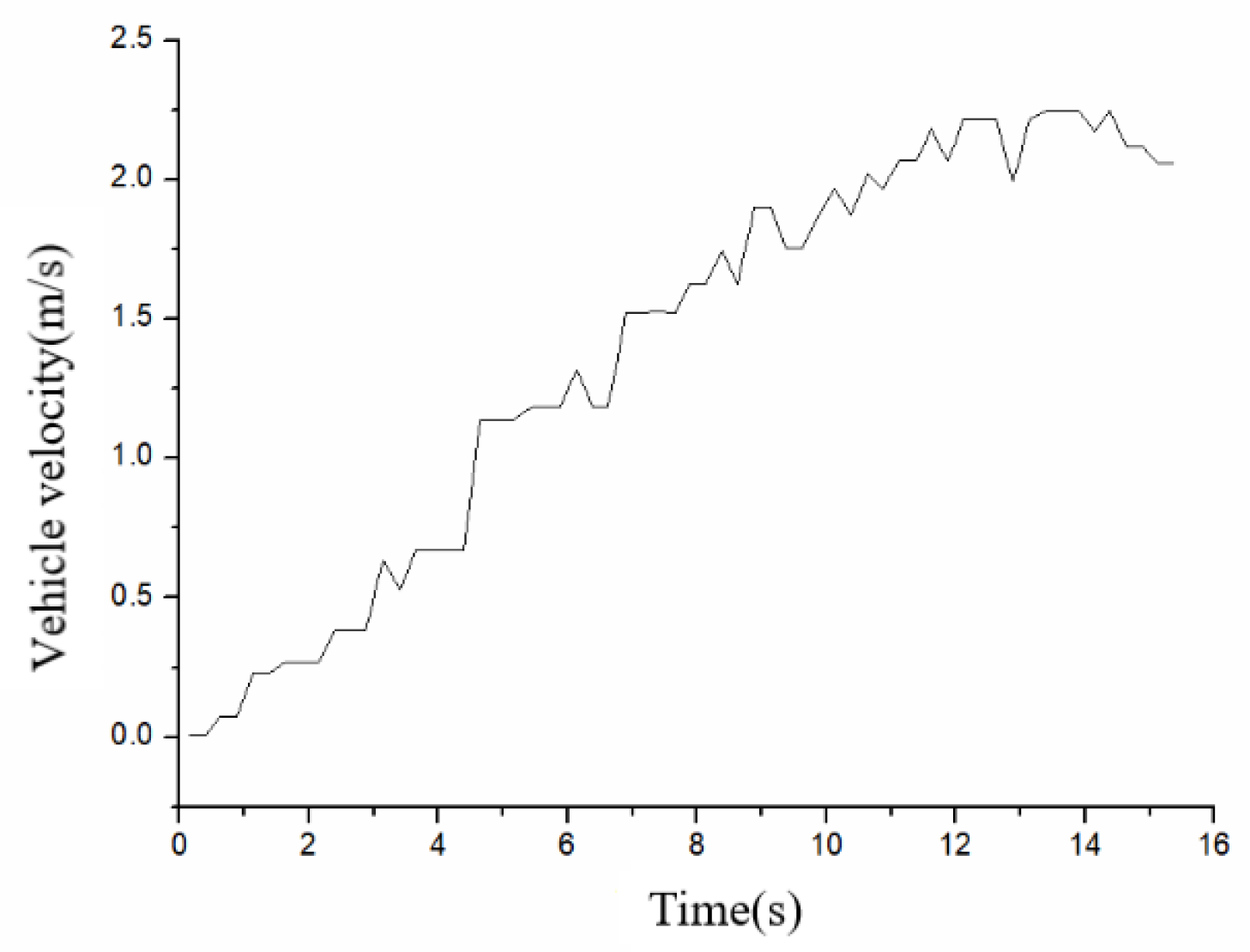
3.1.1. Test of Non-Controlled Strategy

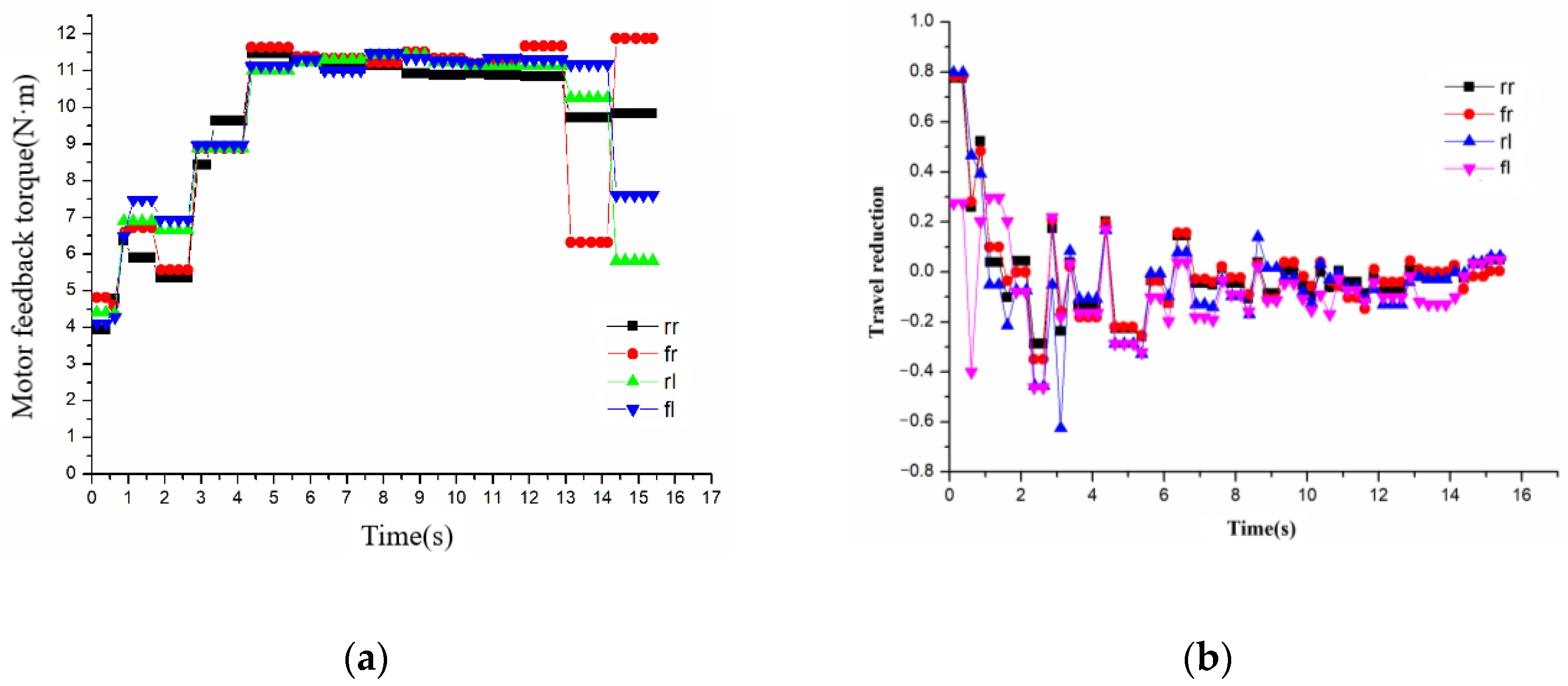
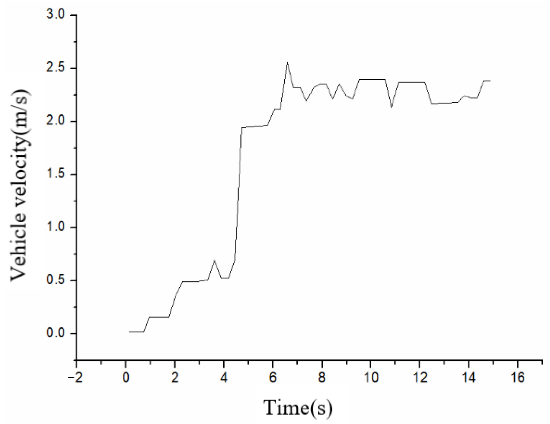
As shown in Figure 7, the vehicle velocity obtained by GPS increased to 2 m/s as. As shown in Figure 8 and Figure 9a, the actual input and feedback torque of the motor, which were obtained by the torque sensor, were similar before t = 13 s. In particular, the difference between the input and the feedback torque became larger when the motor reached the maximum speed. As shown in Figure 9b, the travel reductions fluctuated significantly when the vehicle was running under the condition of the given input torque. At t = 8 s, travel reductions of the four wheels still did not come to be same.

3.1.2. Test of SMC

The target travel reduction was selected as 0.08, and the vehicle speed exceeded 1 m/s at t = 5 s, as shown in Figure 10. The travel reductions of the four wheels were similar to 0.08 after t = 5 s, as shown in Figure 11. Therefore, the travel reductions exceeded the set range of 0–0.2, and the vehicle started to run in straight under SMC at t = 5 s.

The vehicle running trajectory is shown in Figure 12. The Gauss projection coordinates of the gate of the identification station (X: 159778, Y: 3557680) were chosen as the origin. R² (goodness of fit, GOF) between walking and expected trajectory was 0.9998.

3.1.3. Test of Incremental PI Control

Similarly, the target travel reduction was selected as 0.08. As shown in Figure 13 and Figure 14, the travel reductions of the four wheels were similar when the vehicle speed exceeded 1 m/s at the third second. Therefore, the vehicle changed to the automatic control mode with incremental PI control after the third second when the travel reductions exceeded the set range of 0–0.2, and the travel reductions became stable at t = 5 s. The vehicle position was represented in the coordinate system, as shown in Figure 15, in which the data were collected by GPS. R² (goodness of fit, GOF) between walking and expected trajectory was 0.9999.

To compare the performance of the three control strategies, three groups of tests were carried out under the same test parameters. The mean and variance of vehicle travel reduction after reaching the target speed were counted to characterize the stability of the system, as shown in

Table 2. Travel reduction feature of the test.

Group	Wheel	Mean			Variance
		Non-Controlled	SMC	Incremental PI	Non-Controlled	SMC	Incremental PI
1	FL	−0.1324	0.0577	0.0136	0.0988	0.0212	0.0054
	RL	−0.0975	0.0554	0.0229	0.0987	0.0242	0.0032
	FR	0.0053	0.0458	0.0351	0.0275	0.0205	0.0025
	RR	−0.0164	0.1299	0.0385	0.0302	0.011	0.0036
2	FL	−0.015	0.048	0.004	0.0524	0.0248	0.0147
	RL	0.0268	0.0555	0.0304	0.0541	0.021	0.0126
	FR	0.053	0.0768	0.0107	0.0703	0.0139	0.0168
	RR	0.0478	0.0679	0.0341	0.0401	0.0189	0.0108
3	FL	−0.0402	0.0836	0.0578	0.0468	0.0113	0.0002
	RL	−0.0481	0.0487	0.0521	0.0622	0.0246	0.0002
	FR	0.0281	0.0975	0.0589	0.0556	0.0167	0.0002
	RR	0.021	0.0801	0.066	0.053	0.0109	0.0004

.

Compared these three experimental results, the travel reduction of the test group with non-control strategy not only had difficulty to approach the target, but also fluctuated remarkably. Therefore, it was difficult for the vehicle to run in a straight state. Although the vehicle of the test group with incremental PI control could almost run straight, the travel reduction was not sufficiently close to the target.

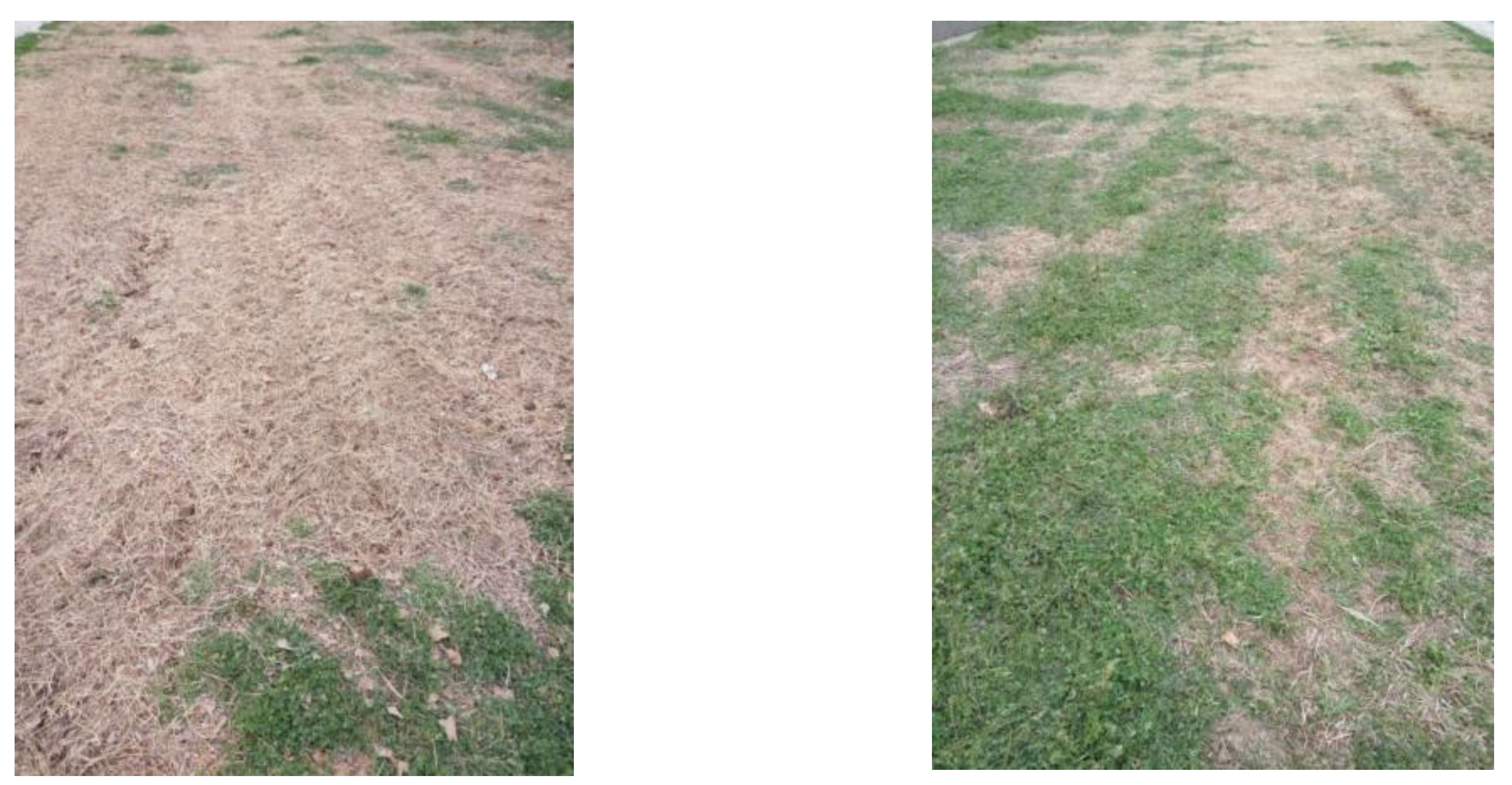
3.2. Separated Pavement Test

For agricultural vehicles, the working environment was regarded as a complicated system, meaning the surfaces under each driving wheel of the vehicle may experience different coefficients of gross tractions and travel reductions. Therefore, the coefficient of gross traction of the wheels must be the same to ensure that the vehicles drive in a straight line. The separated road is shown in Figure 16. The right side of the vehicle was a dirt surface covered with grass, and the left was a concrete surface.

According to Figure 5, the peak coefficient of gross tractions of the right and left surfaces were different, which means that current coefficients of the two sides may be different, although their travel reductions were almost identical. Therefore, to maintain the straight-line driving ability of the vehicle, the coefficient of gross tractions of the wheels should be the same.

3.2.1. Test of Non-Controlled Strategy

Compared to Figure 7, Figure 17a showed that the velocity of the right wheels was significantly lower than that of the left wheels—especially, the right front wheel was the lowest before t = 7 s, which means that the vehicle started to deviate rightward to the grass surface as it ran. When t = 9 s, the velocities of the four wheels were almost the same. The vehicle finally entered the grass surface, completely breaking away from the concrete surface. By collecting the GPS coordinates of each test, the trajectory line is as shown in Figure 18. R² (goodness of fit, GOF) between walking and expected trajectory was 0.8421.

3.2.2. Test of SMC

As shown in Figure 6, travel reductions of right side were set to 0.08, and the left side was set to 0.03, which means that travel reductions of two sides were same. Travel reduction and coefficients of gross traction of the wheels can be shown in Figure 19. If the coefficients tend to be same, the drive torques of each wheel are the same, guaranteeing that the vehicle drives in a straight line. According to the X-Y coordinate axis collected by GPS, the trajectory line is as shown in Figure 20. R² (goodness of fit, GOF) between walking and expected trajectory was 0.9902.

3.2.3. Test of Incremental PI Control

The incremental PI control algorithm was used to control the vehicle, and the travel reduction is shown in Figure 21a.

As shown in Figure 21b, it can be seen that the coefficients were not stable. Furthermore, although travel reduction of all wheels were close to a value of 0.08, only the coefficients of right wheels were close to the target value, which meant that vehicle could not run in a straight. The real trajectory can be seen from the GPS coordinates, as shown in Figure 22. R² (goodness of fit, GOF) between walking and expected trajectory was 0.7642.

3.3. Discussions

In uniform surfaces test, as can be seen from Figure 11 and Figure 14, the vehicle controlled by two algorithms can run with the target travel reduction, compared with non-control strategy. As shown in Figure 12 and Figure 15 and Table 2, although both of them can travel in a straight line, incremental PI control has less settling time and variance.

In separated surfaces test, owing to the different coefficients of gross traction on both sides, the vehicle with non-control strategy was unable to drive in a straight line although the travel reduction on both sides was the same, as shown in Figure 17b and Figure 18. Therefore, when driving on separated surfaces, current coefficients are also necessarily calculated to estimate the peak coefficients, and then control the travel reduction. As can be seen from Figure 19a and Figure 21a, although the settling time of incremental PI control is smaller than that of SMC, SMC has less oscillation than incremental PI control, which can be seen from Figure 19b and Figure 21b. Hence, its driving trajectory is closer to the desired straight line with R² = 0.9902, while R² of incremental PI control is 0.7642, obtained from Figure 20 and Figure 22. Therefore, SMC can remarkably maintain straight driving, when the vehicle is operating on complex surfaces.

Compared with studies [2,3,23] which had not classified surfaces to control DDAVs operating, the two strategies proposed in this article can remarkably enhance the performance so that DDAVs drive in a straight line, which will improve the operation efficiency. Furthermore, running on simple surfaces or uniform surfaces, such as transferring and transportation, DDAVs can enter the straight-line driving state faster under incremental PI control. Due to the faster response time, this can reduce the time for adjusting the vehicle statement and help obtain a higher work efficiency. Running on complicated surfaces or separated surfaces, such as field operation, DDAVs can accurately maintain straight driving under SMC to reduce the deviation of the vehicle and improve the operation efficiency.

4. Conclusions

In this study, a travel reduction control strategy based on SMC and incremental PI control was designed to solve the energy consumption problem caused by excessive slip in the operation process of DDEAVs. The tests of uniform and separated surfaces showed the following:

(1)

According to the difference between the state variables and the target travel reduction, the strategy can effectively distribute the energy and hence driving force of each wheel, so that the travel reduction of the vehicle can be stabilized around the target travel reduction.

(2)

Compared with the non-control strategy, the two strategies can effectively reduce the impact of road changes on vehicle velocity.

(3)

On a uniform surface, the travel reduction of each wheel can be maintained at the target value by using the incremental PI control strategy, with a less settling time.

(4)

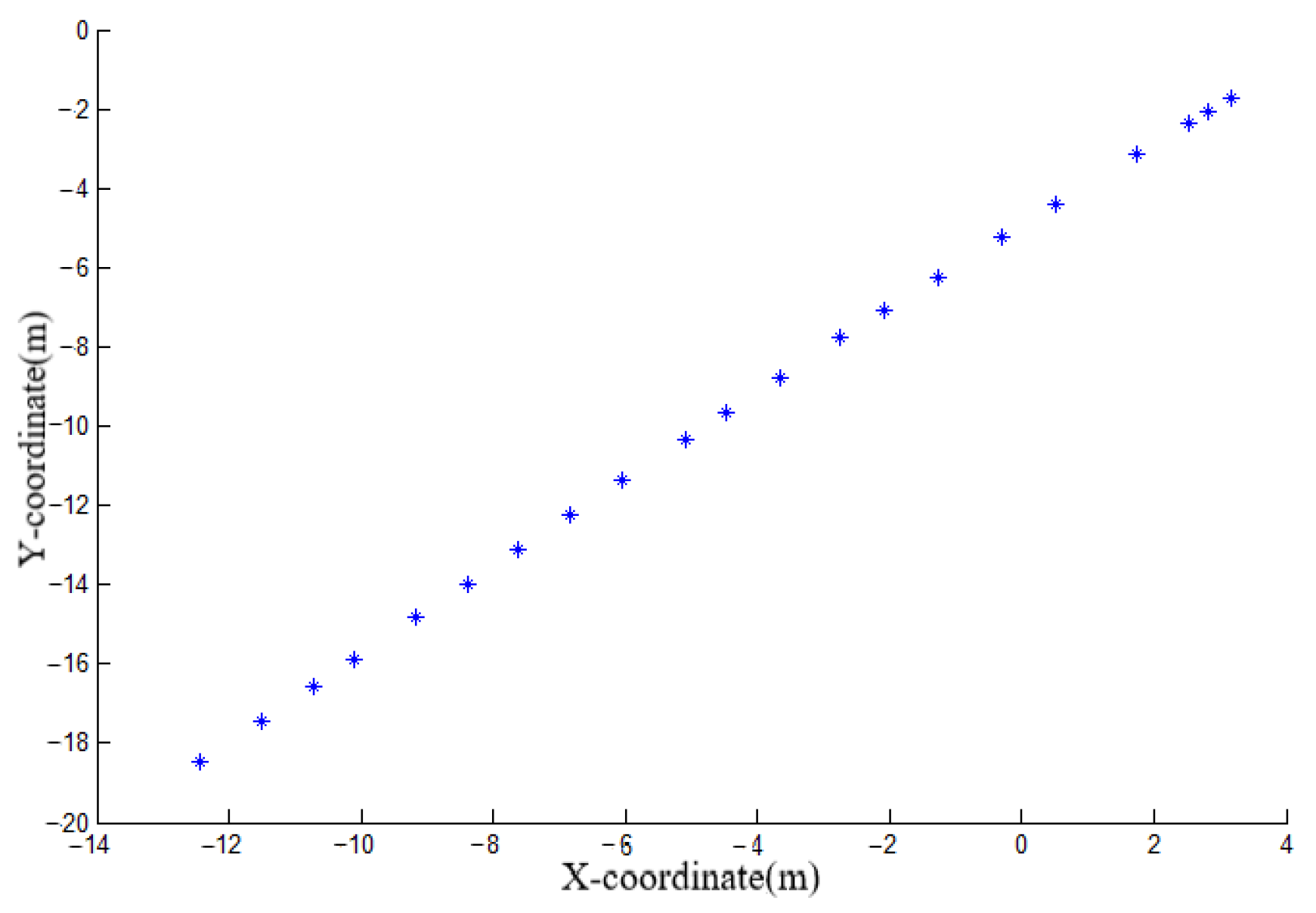
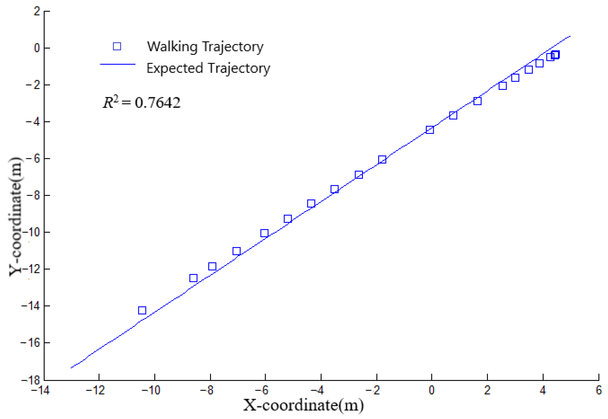
On a separated surface, the travel reduction of each wheel can be maintained at the target value by using the SMC strategy, with less oscillation. The goodness of fit between walking and expected trajectory was 0.9902, which meant its driving trajectory was closer to the desired straight line.

This study can provide a method for the drive control of DDAVs to adapt to more surfaces and meet different operation requirements.

References

1. Zhang, C.B.; Yu, Y.C.; Wu, Y.P. Design of high trafficability four wheel self-propelled field machine for tobacco. Trans. Chin. Soc. Agric. Eng. 2011, 27, 37–41. (In Chinese) [Google Scholar] [CrossRef]
2. Zhang, J.; Chen, D.; Wang, S.M.; Hu, X.A.; Wang, D. Design and experiment of four-wheel independent steering driving and control system for agricultural wheeled robot. Trans. Chin. Soc. Agric. Eng. 2015, 31, 63–70. (In Chinese) [Google Scholar] [CrossRef]
3. Zhang, T.M.; Huang, H.; Huang, P.H. Design and test of drive and control system for electric wheeled mobile car. Trans. Chin. Soc. Agric. Eng. 2014, 30, 11–18. (In Chinese) [Google Scholar] [CrossRef]
4. Wang, Y.; Fujimoto, H.; Hara, S. Driving force distribution and control for EV with four in-wheel motors: A case study of acceleration on split-friction surfaces. IEEE Trans. Ind. Electron. 2017, 64, 3380–3388. [Google Scholar] [CrossRef]
5. Lenzo, B.; Bucchi, F.; Sorniotti, A. On the handling performance of a vehicle with different front-to-rear wheel torque distributions. Veh. Syst. Dyn. 2019, 57, 1685–1704. [Google Scholar] [CrossRef]
6. Cao, Q.M.; Zhou, Z.L.; Zhang, M.Z.; Xi, Z. Algorithm and verification for estimating tractor driving wheel slip rate. Trans. Chin. Soc. Agric. Eng. 2015, 31, 35–41. (In Chinese) [Google Scholar] [CrossRef]
7. Osinenko, P.V.; Geissler, M.; Herlitzius, T. A method of optimal traction control for farm tractors with feedback of drive torque. Biosyst. Eng. 2015, 129, 20–33. [Google Scholar] [CrossRef]
8. Li, H.L.; Luo, Y. T Integrated coordination control for distributed drive electric vehicle trajectory tracking. Int. J. Automot. Technol. 2020, 21, 1047–1060. [Google Scholar] [CrossRef]
9. Beal, C.E.; Gerdes, J.C. Model predictive control for vehicle stabilization at the limits of handling. IEEE Trans. Control. Syst. Technol. 2013, 21, 1258–1269. [Google Scholar] [CrossRef]
10. Choi, M.; Choi, S.B. Model predictive control for vehicle yaw stability with practical concerns. IEEE Trans. Veh. Technol. 2014, 63, 3539–3548. [Google Scholar] [CrossRef]
11. Zhao, Y.; Zhang, C.N. Electronic Stability Control for Improving Stability for an Eight In-Wheel Motor-Independent Drive Electric Vehicle. Shock. Vib. 2019, 2019, 1–21. [Google Scholar] [CrossRef] [Green Version]
12. Zhai, L.; Sun, T.; Wang, J. Electronic stability control based on motor driving and braking torque distribution for a four in-wheel motor drive electric vehicle. IEEE Trans. Veh. Technol. 2016, 65, 4726–4739. [Google Scholar] [CrossRef]
13. Sun, Z.; Xie, H.; Zheng, J.C. Path-following control of Mecanum-wheels omnidirectional mobile robots using nonsingular terminal sliding mode. Mech. Syst. Signal. Process. 2021, 147, 107128. [Google Scholar] [CrossRef]
14. Sun, Z.; Zheng, J.; Man, Z.; Wang, H. Robust control of a vehicle steer-by-wire system using adaptive sliding mode. IEEE Trans. Ind. Electron. 2016, 63, 2251–2262. [Google Scholar] [CrossRef]
15. Chen, S.Y.; Gong, S.S. Speed tracking control of pneumatic motor servo systems using observation-based adaptive dynamic sliding-mode control, Mech. Syst. Signal Process. 2017, 94, 111–128. [Google Scholar] [CrossRef]
16. Li, S.; Wu, C.; Sun, Z. Design and implementation of clutch control for automotive transmissions using terminal-sliding-mode control and uncertainty observer, IEEE Trans. Veh. Technol. 2016, 65, 1890–1898. [Google Scholar] [CrossRef]
17. Feng, Y.; Zheng, J.; Yu, X.; Truong, N.V. Hybrid terminal sliding-mode observer design method for a permanent-magnet synchronous motor control system. IEEE Trans. Ind. Electron. 2009, 56, 3424–3431. [Google Scholar] [CrossRef]
18. Zhou, X.S.; Zhou, J. The tracking control study of distributed electric-driven agricultural vehicles based on real-time online estimation. Adv. Mech. Eng. 2019, 11, 1–12. [Google Scholar] [CrossRef] [Green Version]
19. Zhou, X.S.; Zhou, J. Data-Driven Driving State Control for Unmanned Agricultural Logistics Vehicle. IEEE Access 2020, 8, 65530–65543. [Google Scholar] [CrossRef]
20. Zhong, W.J.; Gao, Q.; Lu, Z.X. Road conditions tractor driving wheel slip ratio of test and analysis. J. Huazhong Agric. Univ. 2015, 34, 130–136. (In Chinese) [Google Scholar]
21. Zhao, L.J.; Deng, N.N.; Ge, Z.H. Real-time road condition estimation for four-wheel-drive vehicle. J. Harbin Inst. Technol. 2014, 46, 42–46. [Google Scholar]
22. Chu, W.B. State Estimation and Coordinated Control for Distributed Electric Vehicles. Ph.D. Thesis, Tsinghua University, Beijing, China, December 2013. [Google Scholar]
23. Zhang, X.J.; Gao, X.H.; Wang, Y.C. Unified dynamical model of vehicle steering and model-following control. Trans. Chin. Soc. Agric. Eng. 2009, 25, 173–177. (In Chinese) [Google Scholar] [CrossRef]
Figure 1. Developed electric distributed drive agricultural vehicle.
Agriculture 12 00070 g001
Figure 2. Hardware structure of the DDAV.
Agriculture 12 00070 g002
Figure 3. Two-wheel simplified model.
Agriculture 12 00070 g003
Figure 4. Relationship of travel reduction and coefficient of gross traction.
Agriculture 12 00070 g004
Figure 5. Relationship between travel reduction and coefficient of gross traction of road surface.
Agriculture 12 00070 g005
Figure 6. Experimental area.
Agriculture 12 00070 g006
Figure 7. Vehicle velocity of non-controlled strategy.
Agriculture 12 00070 g007
Figure 8. Motor output torque of non-controlled strategy.
Agriculture 12 00070 g008
Figure 9. Motor feedback torque and travel reduction of non-controlled strategy.(a) Motor feedback torque; (b) Travel reduction.
Agriculture 12 00070 g009
Figure 10. Vehicle velocity with SMC.
Agriculture 12 00070 g010
Figure 11. Travel reduction of SMC.
Agriculture 12 00070 g011
Figure 12. X-Y coordinates of SMC.
Agriculture 12 00070 g012
Figure 13. Speed of incremental PI strategy.
Agriculture 12 00070 g013
Figure 14. Travel reduction of incremental PI strategy.
Agriculture 12 00070 g014
Figure 15. X-Y coordinates of incremental PI strategy.
Agriculture 12 00070 g015
Figure 16. Test of separated road.
Agriculture 12 00070 g016
Figure 17. Wheel velocity and travel reduction of non-controlled strategy. (a) Wheel velocity; (b) Travel reduction.
Agriculture 12 00070 g017
Figure 18. X-Y coordinates of non-controlled strategy.
Agriculture 12 00070 g018
Figure 19. Travel reduction of and coefficient of gross traction SMC. (a) Travel reduction; (b) Coefficient of gross traction.
Agriculture 12 00070 g019
Figure 20. X-Y coordinates of SMC.
Agriculture 12 00070 g020
Figure 21. Travel reduction and coefficient of gross traction of incremental PI strategy. (a) Travel reduction; (b) Coefficient of gross traction.
Agriculture 12 00070 g021
Figure 22. X-Y coordinates of incremental PI strategy.
Agriculture 12 00070 g022