Abstract
Efficient monitoring of cultivated land quality (CLQ) plays a significant role in cultivated land protection. Soil spectral data can reflect the state of cultivated land. However, most studies have used crop spectral information to estimate CLQ, and there is little research on using soil spectral data for this purpose. In this study, soil hyperspectral data were utilized for the first time to evaluate CLQ. We obtained the optimal spectral variables from dry soil spectral data using a gradient boosting decision tree (GBDT) algorithm combined with the variance inflation factor (VIF). Two estimation algorithms (partial least-squares regression (PLSR) and back-propagation neural network (BPNN)) with 10-fold cross-validation were employed to develop the relationship model between the optimal spectral variables and CLQ. The optimal algorithms were determined by the degree of fit (determination coefficient, R2). In order to estimate CLQ at the regional scale, HuanJing-1A Hyperspectral Imager (HJ-1A HSI) data were transformed into dry soil spectral data using the linkage model of original soil spectral reflectance to dry soil spectral reflectance. This study was conducted in the Guangdong Province, China and the Conghua district within the same province. The results showed the following: (1) the optimal spectral variables selected from the dry soil spectral variables were 478 nm, 502 nm, 614 nm, 872 nm, 966 nm, 1007 nm, and 1796 nm. (2) The BPNN was the optimal model, with an R2(C) of 0.71 and a normalized root mean square error (NRMSE) of 12.20%. (3) The results showed the R2 of the regional-scale CLQ estimation based on the proposed method was 0.05 higher, and the NRMSE was 0.92% lower than that of the CLQ map obtained using the traditional method. Additionally, the NRMSE of the regional-scale CLQ estimation base on dry soil spectral variables from HJ-1A HSI data was 2.00% lower than that of the model base on the original HJ-1A HSI data.
1. Introduction
Due to rapid socio-economic development and urbanization, the amount of cultivated land in China has been decreasing. Cultivated land quality (CLQ) is an agriculture land quality grade that represents the soil fertility and natural conditions of cultivated land [1,2]. Cultivated land quality evaluation is crucial to ensuring the sustainability of cultivated land [3,4]. Traditional CLQ evaluations have primarily relied on field investigations and laboratory analyses, although these methods are not well suited for real-time dynamic monitoring of CLQ [5,6,7].
With the steady growth of remote sensing, several scholars have utilized remote sensing techniques to evaluate CLQ in recent years [8,9,10]. The methods can be divided into two categories: the quasi-satellite-driven CLQ evaluation method and the satellite-driven CLQ evaluation method. In the quasi-satellite-driven CLQ evaluation method, the indicators were divided into two components by the traditional CLQ assessment system (GB/T 28407-2012): some indicators were acquired from field investigations and laboratory analyses, while others were obtained from remote sensing data. For instance, Yang et al. (2012) obtained the soil organic matter (SOM) content and soil pH from field measurements and developed a model to relate the information to Landsat TM5 data to establish a CLQ evaluation method [11]. Yu et al. (2012) established a CLQ evaluation indicator system using soil nutrient content and topsoil thickness obtained from field measurements and MODIS data [12]. However, the other indicators in the method cannot be obtained from remote sensing data, making rapid and timely monitoring of CLQ difficult or impossible.
In satellite-driven CLQ evaluation methods, vegetation indicators are used to estimate CLQ. For example, Zhu et al. (2020) used the empirical Bayesian kriging (EBK) algorithm to scale down the MODIS gross primary productivity (GPP) data of rice in different growth periods and constructed a CLQ evaluation model based on GPP [13]. Guan et al. (2018) established a CLQ evaluation model based on the normalized difference vegetation index (NDVI) from Landsat data modified by grain yield data [14]. These methods focused on the relationship between the spectral response of vegetation and CLQ, overcoming the limitations of the quasi-satellite-driven CLQ evaluation method. However, the spectral response of the crop affects the CLQ estimation, and different crops with different spectral responses will result in different CLQ estimates, resulting in potentially large errors.
In contrast, soil spectral data can provide CLQ estimates unaffected by the crop spectral response. In recent years, hyperspectral data have been increasingly used to obtain the physical and chemical characteristics of soil [15,16]. The goal of this study is to develop a novel method to estimate CLQ using soil spectral data [10,13]. The objectives are to (1) determine the optimal spectral variables describing the correlation between soil spectral data and CLQ; (2) establish a CLQ evaluation model based on the optimal spectral variables; (3) expand the model to regional-scale CLQ estimation using HuanJing-1A Hyperspectral Imager (HJ-1A HSI) data.
2. Materials and Methods
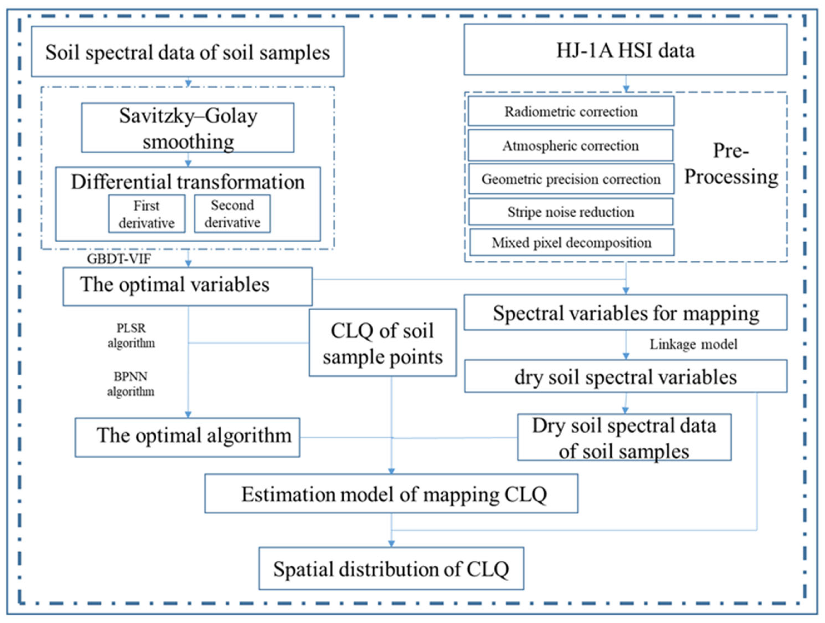
In this study, the soil hyperspectral technique was utilized to evaluate CLQ. The flowchart of the method is shown in Figure 1. First, we selected the optimal spectral variables of dry soil samples using the GBDT–VIF method. Secondly, comparing PLSR to BPNN algorithms, the optimal algorithm was determined using the 10-fold cross-validation method. Thirdly, HJ-1A data were transformed into spectral values of dry soil using the linkage model. Then, the relationship model between CLQ and the spectral variables of dry soil samples was constructed. Finally, regional-scale CLQ using HJ-1A data was estimated based on the relationship model.
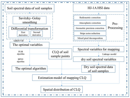
Figure 1.
The flowchart of method.
2.1. Study Area
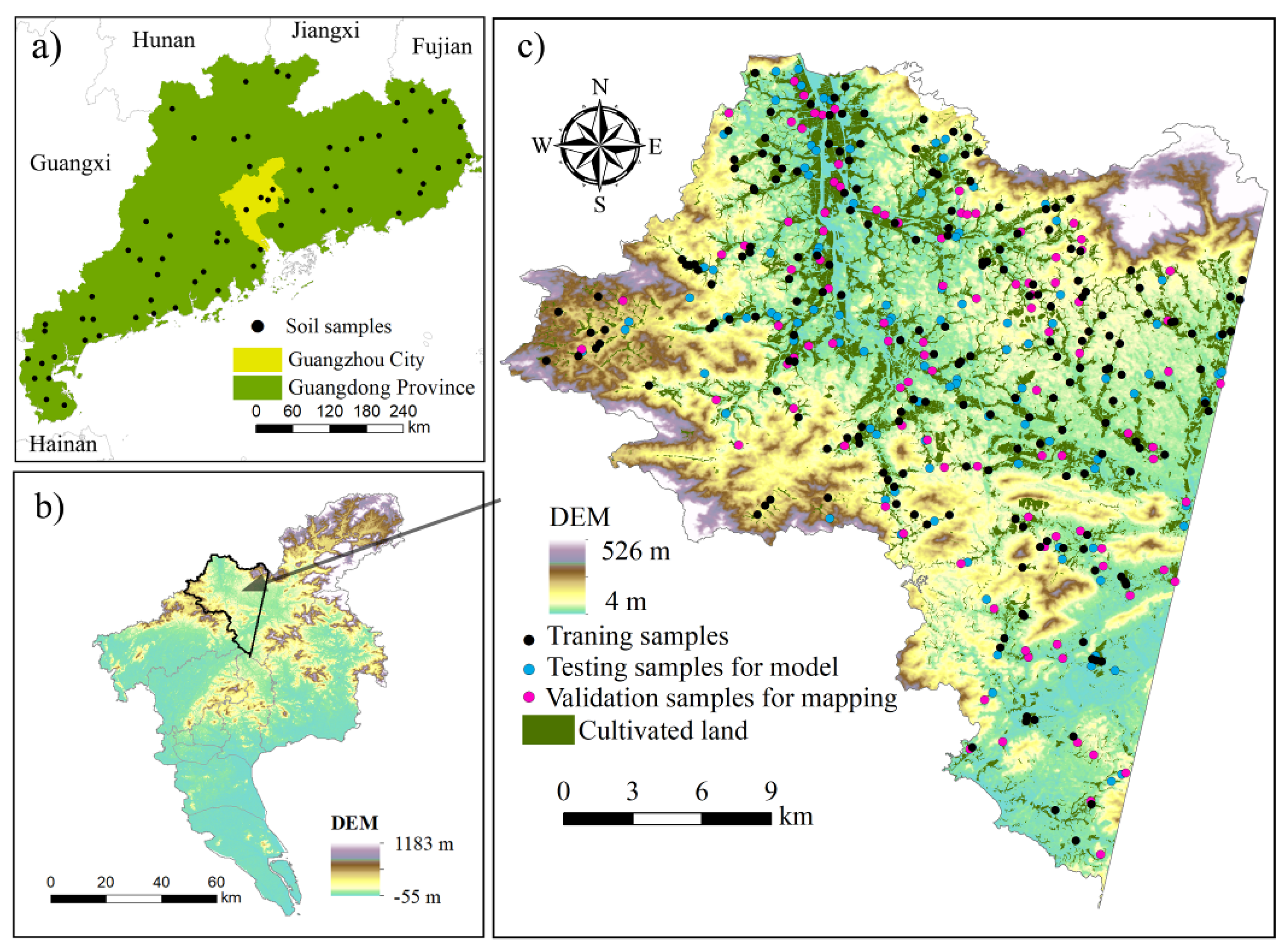
As one of the rapidly developing urban areas in China, the CLQ in Guangdong province often changes dramatically due to the influence of anthropogenic and environmental factors [13]. Thus, we selected Guangdong province as the study area for establishing the CLQ estimation model (20°09′~25°31′ N, 109°45′~117°20′ E) (Figure 2a). Referring to the Guangdong Statistical Yearbook in 2021, the area has an average of 1767 h of sunshine, an annual average temperature of 22.8 °C, and annual precipitation of 1505 mm. Guangdong Province is an important grain production area in China, with a cultivated land area of 4.28 × 10⁴ km2. The study area for the regional-scale CLQ estimation was the Conghua district within Guangzhou City (Figure 2b). The area of cultivated land in Conghua covers 2.05 × 10² km2.

Figure 2.
(a) Location of Guangdong province with the soil sampling distribution; (b) the DEM of the study area in Guangzhou city; (c) the distribution of samples for regional-scale CLQ estimation in the Conghua district (the plots for model training are black, the plots for mapping model testing are blue, and the plots for mapping accuracy validation are pink).
2.2. Data and Pre-Processing
2.2.1. Samples Data
A total of 71 topsoil (0~20 cm) samples (approximate weight of 300 g) of cultivated land were collected in a sampling grid (50 km × 50 km) in Guangdong province (Figure 2a) to establish the CLQ estimation model. The area of the sample plot was the same as the spatial resolution of the HJ-1A HSI image (100 m × 100 m). The five-point sampling method was adopted for soil collection—that is, the midpoint of the diagonal of the sample plot was the central sampling point, and the remaining four sample points were located in the center of the 4 quadrats of the sample plot. The GPS coordinates of the sampling plots were obtained [17].
To remove stones and other debris, the soil samples were air-dried at an ambient temperature for three days and sieved through a 2 mm polyethylene sieve. After that, using an agate mortar, the soil samples were ground into fine particles. Before measuring the soil spectral reflectance, the ground soil samples were processed through a 20-mesh sieve (0.84 mm) to obtain a relatively homogeneous particle size and oven dried for 24 h at 105 °C [18].
Moreover, CLQ and spectral data from HJ-1A data at 400 sample points designed using a stratified sampling method were collected in the Conghua district within Guangzhou City for estimating and validating CLQ at the regional scale (Figure 2c).The samples were randomly divided into three groups: 200 samples (black plots in Figure 2c) were used to build a model for estimating CLQ at the regional scale, 100 samples (blue plots in Figure 2c) were used for model testing, and another 100 samples (pink plots in Figure 2c) were used for accuracy validation for regional CLQ estimation. In this study, the CLQ data of the samples were obtained from the CLQ map dataset of the Department of Natural Resources of Guangdong Province.
2.2.2. Spectral Data Acquisition and Pre-Processing
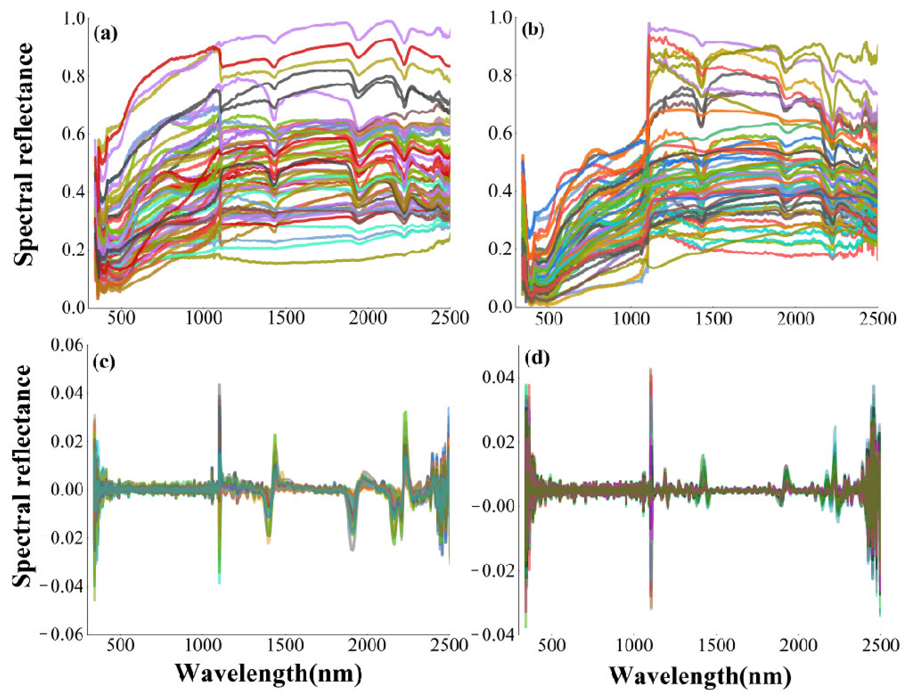
The spectral data of the soil samples were measured using an AvaField portable spectrometer (Avantes, Inc., Apeldoorn, The Netherlands) with a band range of 340–2511 nm and a sampling interval of 0.6 nm. The soil samples were put in a dark room, and a 50 W halogen lamp with a 10° field of view was employed to simulate sunshine. The optical probe was located about 0.15 m above the soil sample [19]. A Savitzky–Golay filter (window size of 10) was used to smooth the spectral data to minimize noise [20,21]. Differential transformation is a common analysis method for processing soil spectral data. It can smooth the signal intensity, reduce the effects of background noise, and improve spectral sensitivity [20,22]. In this study, the spectral data of the dry soil were processed using the first derivative (FD) and second derivative (SD) (Figure 3).
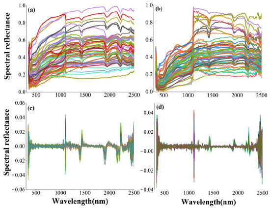
Figure 3.
The spectral variables curves: (a) original soil spectral curves; (b) dry soil spectral curves; (c) the first derivative spectral curves; (d) the second derivative spectral curves.
The HJ-1A HSI data were used to apply the CLQ estimation model to the regional scale in the Conghua district. The image was obtained on 30 October 2017 with a 100 m spatial resolution, and it contained 115 bands (459–956 nm). In this study, HJ-1A HSI was pre-processed (radiometric correction, atmospheric correction, geometric correction, and stripe noise reduction) in ENVI 5.3 software (Exelis Visual Information Solution, Inc., Boulder, CO, USA).
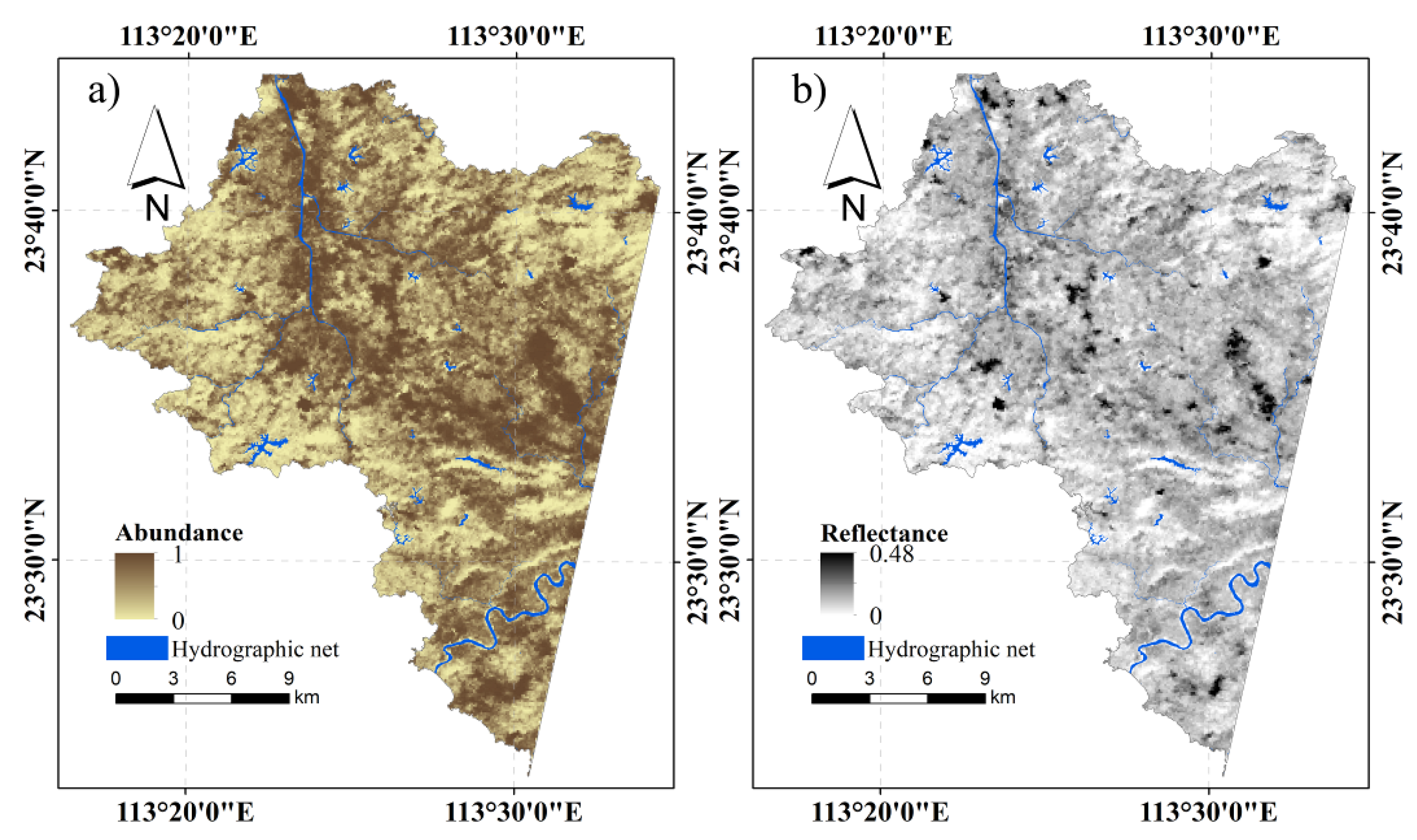
Since mixed pixels existed in HJ-1A HSI data with 100 m spatial resolution, fully constrained least squares (FCLS) linear spectral mixture analysis was used to obtain pure pixels (Figure 4). The equations of this method are defined as [23]:
where is the abundances of the soil endmembers, is the pure vegetation pixels reflectance values, is the pure soil pixels reflectance values, is the mixed pixels reflectance values, and is used to constrain mixed pixels.
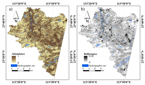
Figure 4.
The result of component decomposition based on FCLS: (a) soil abundance; (b) soil spectral reflectance at 900 nm of the HJ-1A HSI data.
2.3. Methods
2.3.1. Selecting the Optimal Spectral Variables of Dry Soil
One of the most important steps in the development of the soil hyperspectral estimation method of CLQ was the determination of the optimal spectral variables. In this study, the feature importance () of spectral variables obtained using the gradient boosting decision tree (GBDT), combined with the variance inflation factor (VIF), was used to select the spectral variables of dry soil. The formula of () is written as [24,25]:
where is the feature importance of the spectral variables in a single tree, is the number of trees, and denotes the spectral variables. is calculated by loss reduction after splitting, expressed as:
where is the number of leaf nodes, is the number of non-leaf nodes, is the feature associated with node , and is the square of the loss value after node splitting. In this study, we selected the spectral variables with > 0.003.
In order to reduce the collinearity, the variance inflation factor (VIF) was used for further selection of optimal spectral variables, and the spectral variables with a VIF within ten will be retained [26].
2.3.2. Determining the Optimal Algorithm for Estimating CLQ
In this study, a linear algorithm (partial least-squares regression (PLSR)) and a nonlinear algorithm (back-propagation neural network (BPNN)) were used to construct CLQ estimation model.
PLSR is an algorithm proposed by Herman Wold that is used for multivariate analysis [27]. This algorithm has been widely used in the field of science and has achieved favorable results because it can describe a relationship if the size of predictors is far larger than that of the training samples [28]. PLSR was used to establish a linear relationship model between the optimal soil spectral variables and CLQ. The PLSR is expressed as:
where is the normalized dependent variable (value of CLQ), is the normalized independent variable (optimal soil spectral variables), is the coefficient matrix, and is the residual matrix.
The BPNN algorithm was applied to describe the nonlinear relationship between the optimal soil spectral variables and CLQ. The algorithm consists of a multi-layer feed-forward network trained by an error back-propagation algorithm [29,30]. The steepest descent method in the BPNN is used to adjust the weights, and the back-propagation algorithm is utilized to minimize the error of the network [31,32]. The BPNN includes three parts: input layer, hidden layer, and output layer. The transfer function from the input layer to the hidden layer can be expressed as:
where is the value of the optimal soil spectral variables; is the hidden layer information; is the weight of the input layer to the hidden layer; is the transfer function from the input layer to the hidden layer (the Trainlm function is selected in this study); is the hidden layer threshold.
The transfer function from the hidden layer to the output layer is written as:
where is the predicted value of CLQ; is the transfer function from the hidden layer to the output layer (the Purelin function is selected in this study); is the weight of the hidden layer to the output layer; is the threshold of the output layer.
To lower the mean square error (MSE) between the predicted and measured values, the Levenberg–Marquardt algorithm was employed to alter the connection weight from the output layer to the input layer. The MSE is expressed as:
where is the measured value of CLQ, is the predicted value of CLQ, and is the number of training samples.
In this study, the determination coefficient (R2, Equation (8)), the normalized root mean square error (NRMSE, Equation (9)), and concordance correlation coefficient (CCC, Equation (10)) were used to assess the performance of the CLQ estimation models. The equations are calculated as [33,34]:
where is the measured CLQ, is the predicted CLQ, is the average value of the measured CLQ, is the average value of the predicted CLQ, and is the number of the samples.
2.3.3. Regional-Scale CLQ Estimation from HJ-1A HSI Data
The optimal CLQ estimation algorithm was applied to estimate the CLQ at the regional scale in the Conghua district using the HJ-1A HSI image. Due to limitations in the wavelength range (459–956 nm) of the HJ-1A imagery, only the optimal spectral variables in this wavelength range were selected to estimate CLQ. Moreover, due to the effects of soil moisture, the spectral variables obtained from the HJ-1A HSI image reflected soil information that differed from the measured dry soil spectral data obtained from the AvaField portable spectrometer [35]. Therefore, a linkage model was adopted to transform the spectral variables obtained from the HJ-1A HSI data into dry soil spectral variables. The linkage model is expressed as [36]:
where is the dry soil spectral reflectance from HJ-1A HSI data, is the spectral reflectance obtained from the HJ-1A imagery, is the soil moisture content obtained from the soil moisture active passive (SMAP) satellite mission data acquired on 30 October 2017, and a and b represent model coefficients [36].
After the selection of the optimal variables, the model-based optimal algorithm was revised to estimate CLQ.
3. Results
3.1. The Selected Optimal Dry Soil Spectral Variables for CLQ Estimation
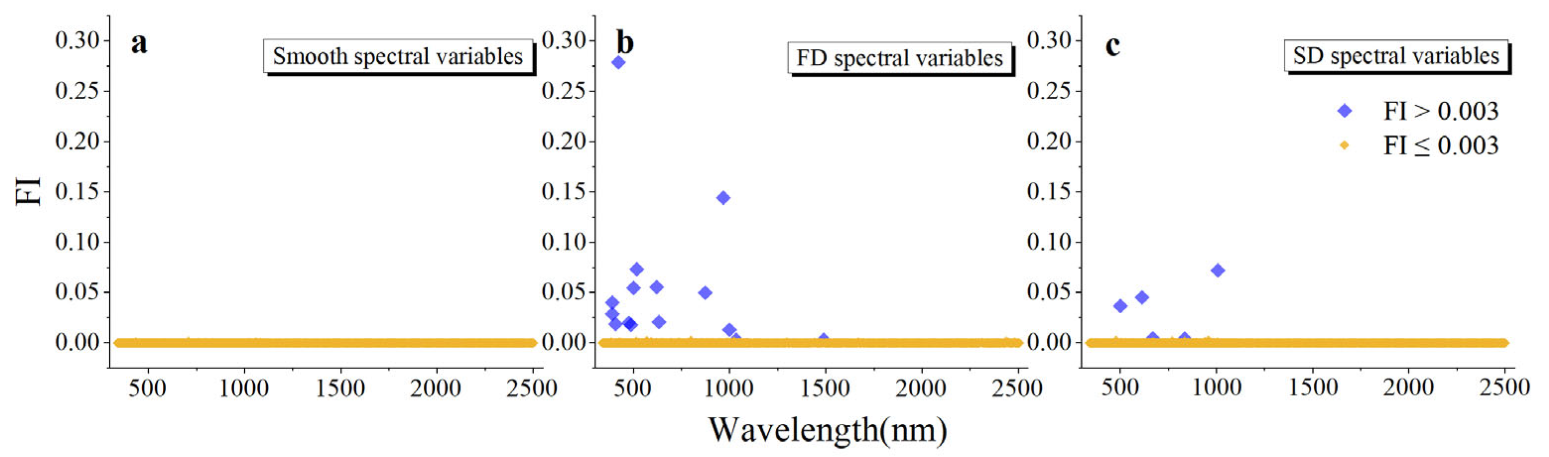
The GBDT algorithm was used to select the optimal spectral variables for estimating CLQ. The feature importance (FI) of the soil spectral variables is shown in Figure 5. Twenty spectral variables were selected (FI > 0.003). Then, the VIF was used to eliminate the collinearity of the above selected spectral variables and the optimal spectral variables (X1:FD478, X2:FD872, X3:FD966, X4:FD1796, X5:SD502, X6:SD614, and X7:SD1007) were obtained, as shown in Table 1.
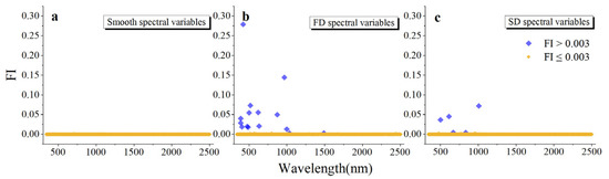
Figure 5.
The feature important of soil spectral variables: (a) smooth spectral variables; (b) first derivative (FD) spectral variables; (c) second derivative (SD) spectral variables.

Table 1.
The optimal spectral variables.
3.2. The Optimal Algorithm for Evaluating CLQ
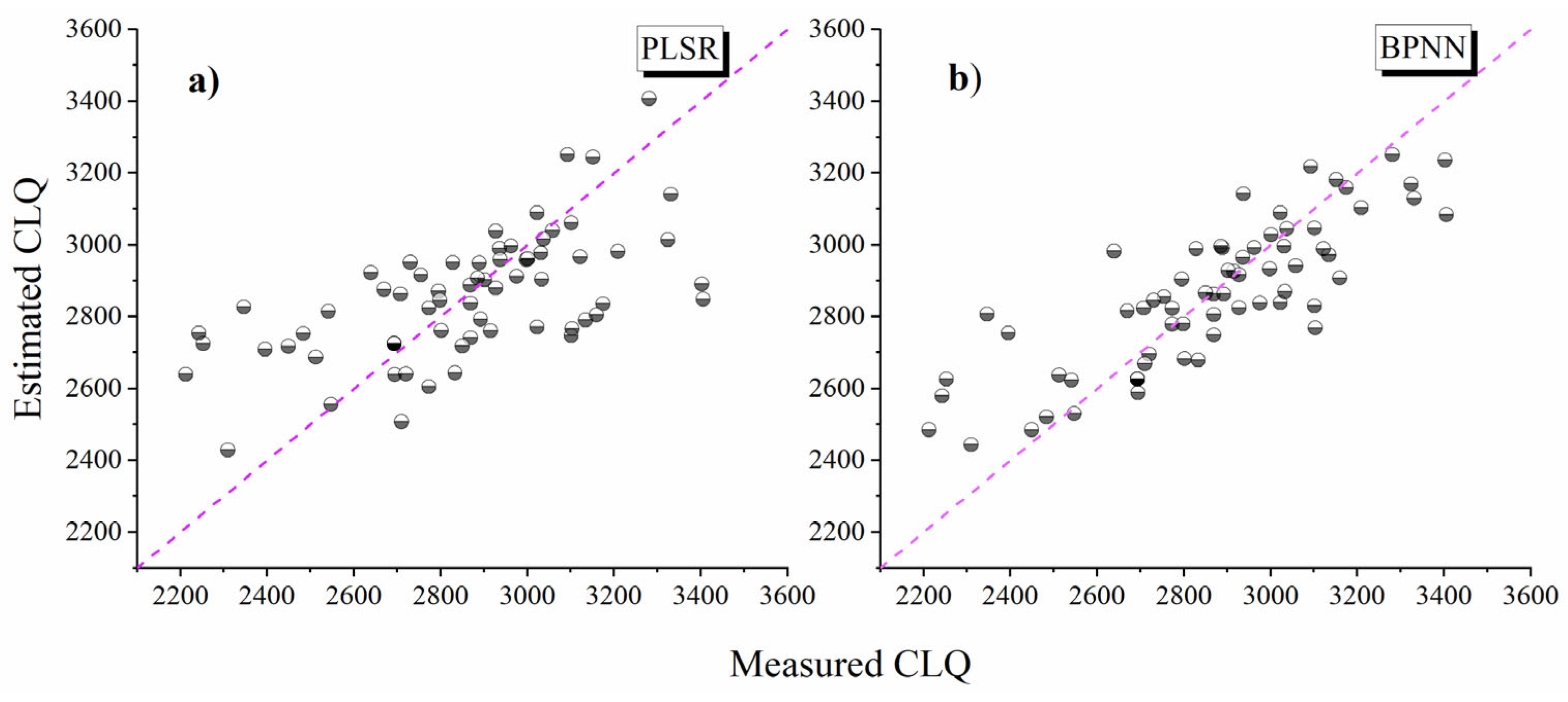
The PLSR and BPNN algorithms were used to construct a relationship model between the optimal spectral variables of dry soil and CLQ. The 71 dry soil samples (black plots in Figure 2a) corresponding to the optimal spectral variables (Table 1) were used as the independent variable, and the value of CLQ was the dependent variable. A 10-fold cross-validation was used to evaluate the performance of the CLQ estimation model. Comparing the PLSR and BPNN, the BPNN model exhibited better performance in cross-validation than the PLSR, with R2(C) of 0.71 (R2CV of 0.67), CCC of 0.79, and NRMSEC of 11.20% (NRMSECV of 12.10%). The R2(C) of the PLSR model was 0.33 lower, and the NRMSEC was 6.73% higher than that of the BPNN (Table 2). The points of the BPNN model in the scatterplot were closer to the 1:1 line than that of the PLSR (Figure 6). The result indicated a nonlinear relationship between the optimal spectral variables of dry soil and the value of CLQ.
Table 2.
Accuracy assessment of estimated CLQ.
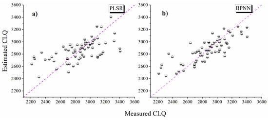
Figure 6.
Scatterplots of measured versus estimated values of CLQ obtained two models: (a) PLSR model; (b) BPNN model.
3.3. Regional-Scale CLQ Estimation Based on HJ-1A Data
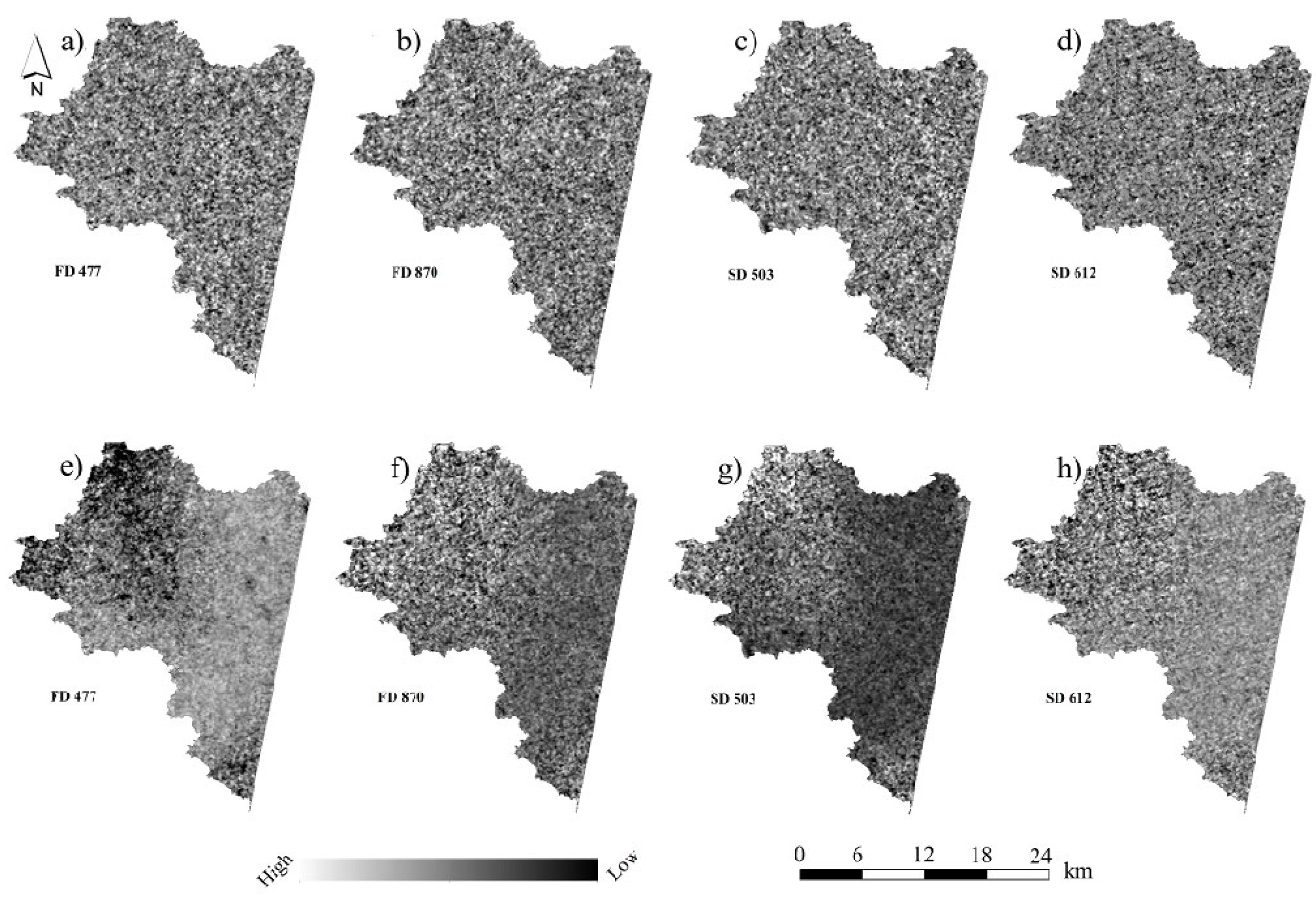
Given the optimal spectral variables and the band range (459–956 nm) of the HJ-1A HSI data, we finally chose four optimal spectral variables (X1:FD477, X2:FD870, X5:SD503, and X6:SD612) to estimate CLQ. According to Equation (11), the four optimal spectral variables obtained from the HJ-1A HSI data were transformed into the dry soil spectral variables, as shown in Figure 7.

Figure 7.
The optimal spectral variables for regional-scale CLQ estimation: (a–d) the spectral variables obtained from HJ-1A HSI data; (e–h) the dry soil spectral variables transformed from HJ-1A HSI data.
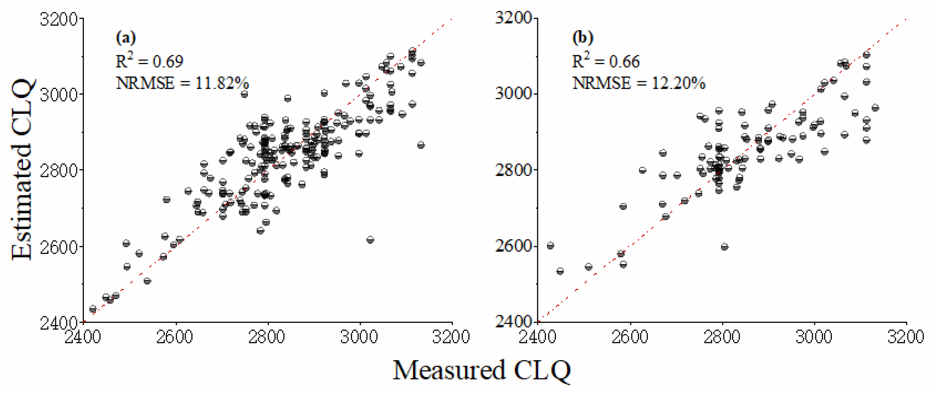
Based on the four dry soil spectral variables transformed above and CLQ in the Conghua district, the BPNN model was reconstructed to estimate CLQ. We used the value of CLQ from 200 training sample points (black plots in Figure 2c) as the dependent variable and the corresponding dry soil spectral variables from the HJ-1A HSI data as independent variables. Figure 8a presents the modeling accuracy of the estimation model, with R2 and NRMSE values of 0.69 and 11.82%, respectively. We used 100 test samples (blue plots in Figure 2c) to validate the model. The R2 of the model was 0.66, and the NRMSE was 12.20%; the majority of the points in the scatterplot were close to the 1:1 line (Figure 8b), indicating the reliability of the model.
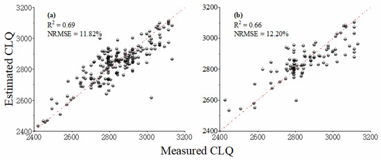
Figure 8.
Scatterplots of measured versus estimated values of CLQ using the (a) training dataset and (b) testing dataset.
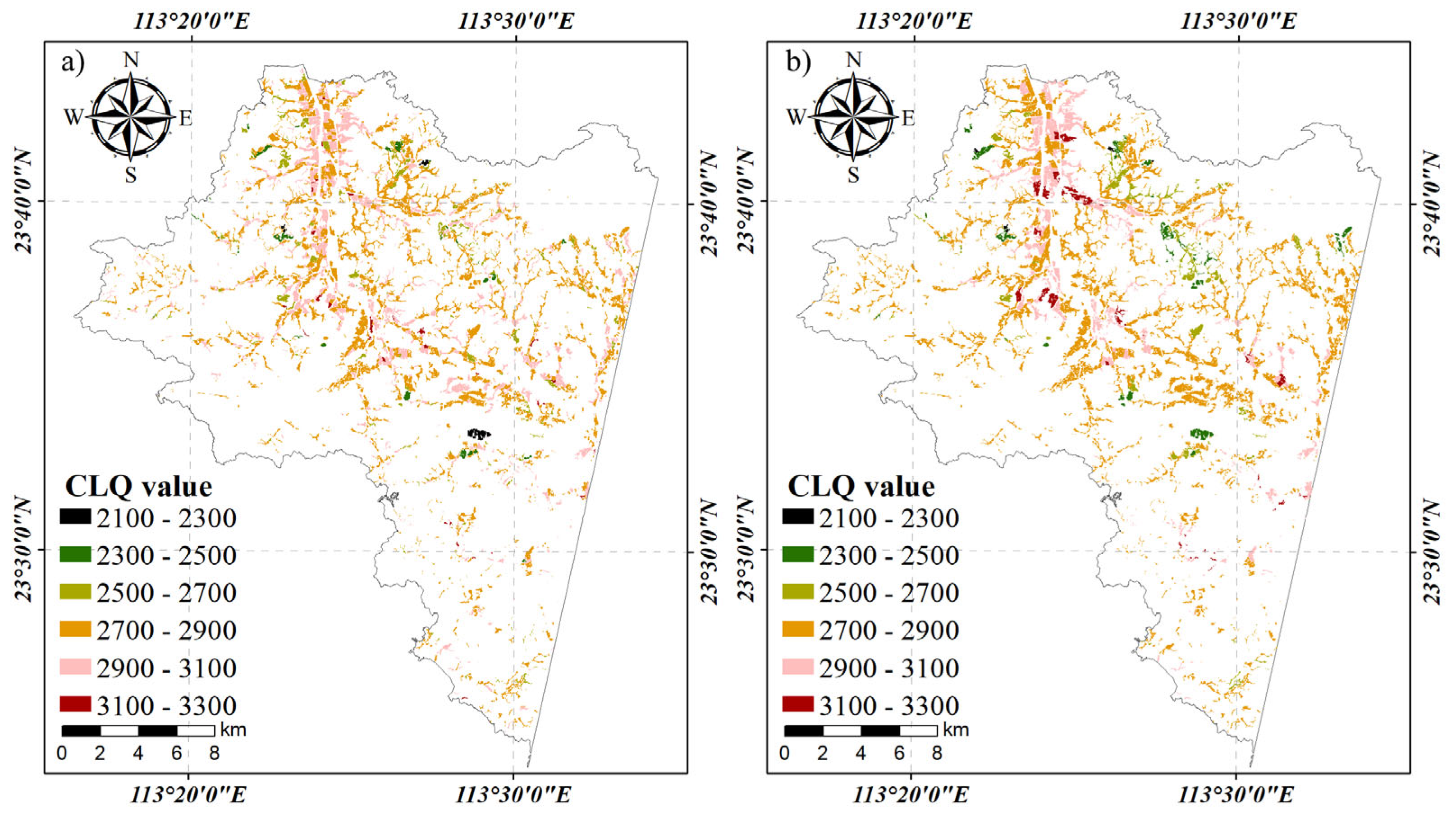
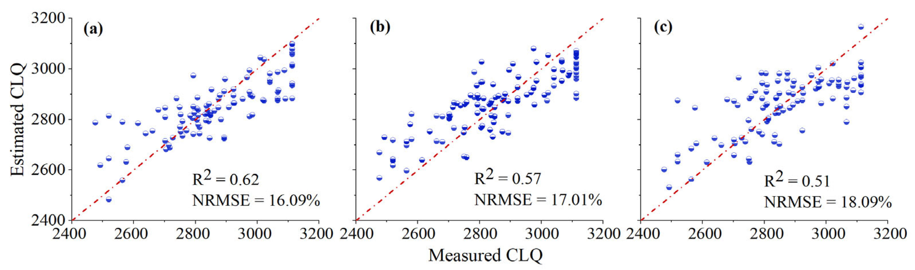
The result of the regional-scale CLQ estimation is presented in Figure 9a. Most of the CLQ values in the study area are between 2700 and 3100. The CLQ values are greater in the north of the study area and lower in the south, which is similar to the trend of the CLQ map obtained using the traditional CLQ assessment method (Figure 9b). 100 sample points (pink point in Figure 2c) were used to calculate the accuracy metrics (R2 and NRMSE), as shown in Figure 10. The results showed that the R2 of the regional-scale CLQ estimation was 0.05 higher, and the NRMSE was 0.92% lower than that of the CLQ map obtained using the traditional CLQ assessment method. Moreover, we compared CLQ estimates using original HJ-1A HSI spectral variables to dry soil spectral variables from HJ-1A HSI data, and the results (Figure 10) showed that the R2 was 0.11 lower and the NRMSE was 2.00% higher for the original HJ-1A HSI spectral variables than the dry soil spectral variables from HJ-1A HSI data. Most of the points in the scatterplot were close to the 1:1 line. The results indicate that the proposed approach has potential for CLQ evaluation.
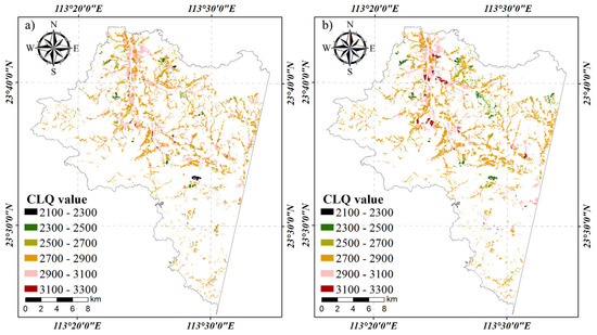
Figure 9.
(a) Spatial distributions of the estimated CLQ; (b) CLQ map obtained using the traditional method.
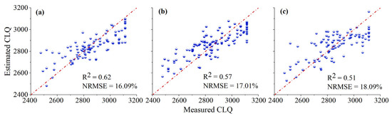
Figure 10.
The measured versus estimated CLQ value (a) based on the proposed method; (b) based on the traditional method; (c) using the original HJ-1A HSI spectral variables.
4. Discussion
CLQ evaluation is crucial for national food security and social stability. Since ground-based CLQ evaluations are time-consuming and costly, several scholars have used remote sensing-based methods. Previous studies focused on crop spectral information to estimate CLQ, however, the results are affected by the crop’s spectral response [7,13]. This study is the first attempt to evaluate CLQ using soil spectral data to reduce the influence of the crop’s spectral information.
The optimal spectral variables (FD478, FD872, FD966, FD1796, SD502, SD614, and SD1007) were selected using the GBDT algorithm and VIF. It was found that some optimal variables (e.g., FD478, FD872, and FD966) were consistent with those of soil nutrients (e.g., FD405–FD483, FD840, FD890, and FD967–FD1031), reflecting CLQ in previous studies [37,38] and indicating that the optimal variables of the dry soil were reliable.
In this study, a linear algorithm (PLSR) and a nonlinear algorithm (BPNN) were used to establish the CLQ estimation model. The BPNN model performed better than the PLSR model, and its R2 was 0.33 higher than that of the PLSR model. This result suggested a nonlinear relationship between the CLQ and the spectral variables, which agrees with previous studies [7].
Previous studies mostly used remote sensing images (e.g., MODIS images) to construct the CLQ estimation model [13]. We developed a CLQ estimation model based on measured dry soil spectral data using an AvaField portable spectrometer. However, the spectral variables from the HJ-1A HSI data were different from the spectral variables from the measured dry soil spectral data. Thus, a linkage model was used to transform the spectral variables obtained from the HJ-1A HSI data into spectral variables corresponding to dry soil to estimate CLQ at the regional scale using the HJ-1A HSI image.
The accuracy of the CLQ estimation was higher when using the dry soil spectral variable than the original image data, indicating the effectiveness of the linkage model. Compared with previous studies (R2 from 0.59 to 0.69) based on vegetation indicators [7,10,13], the accuracy of CLQ estimation was improved with R2 of 0.71, indicating that the proposed method has potential for estimating CLQ. In addition, the R2 of the regional-scale modeling was lower (R2 = 0.69) than that of the model using the dry soil spectral variables obtained from the measured spectral data (R2 = 0.71). The reason is the limitation in the wavelength range (459 to 956 nm) of the optimal spectral variables for estimating CLQ at the regional scale.
5. Conclusions
In this study, soil spectral data were used for the first time to estimate CLQ. This study was conducted in the Guangdong province and Conghua district within the province and led to the following conclusions: the GBDT combined with the VIF accurately selected the optimal spectral variables of the dry soil. The nonlinear model performed better than the linear model for estimating CLQ, indicating a nonlinear relationship between the soil spectral data and CLQ. The use of the dry soil spectral variables from the HJ-1A HSI data resulted in a 2.00% lower NRMSE than the use of the original HJ-1A HSI data. The result indicated that the proposed approach could more accurately estimate CLQ than other methods based on original imagery data.
In this study, a relatively small sample size (71 dry soil samples) was used to construct and validate the estimation models. However, the dry soil samples were used to determine the optimal spectral variables and optimal algorithm rather than performing spatial CLQ estimation. Thus, the sample size was statistically acceptable. In the next study, a larger sample size will be used for establishing and validating the estimation methods. Moreover, field measured hyperspectral data will be introduced, and the linkage model in conjunction with hyperspectral data in the laboratory, field measured hyperspectral data, and remote sensing imagery will be applied to improve CLQ estimation accuracy.
We used the BPNN model to estimate CLQ, however, the initial parameters of the BPNN model are uncertain (such as the number of neuron nodes). An incorrect parameter setting may lead to overfitting or underfitting of the model, potentially affecting the model’s accuracy. Therefore, we will add parameter optimization algorithms (such as the particle swarm optimization algorithm) to improve the efficiency and stability of the BPNN model in the next stage of the study.
Author Contributions
Conceptualization, C.L. and Y.H.; methodology, C.L. and Z.L.; software, C.L.; validation, Y.H., Y.P., Z.L. and D.P.; investigation, C.L. and Y.P.; resources, L.W. and Y.H.; data curation, C.L., L.W. and Y.P.; writing—original draft preparation, C.L.; writing—review and editing, C.L. and Z.L.; funding acquisition, Y.H. and L.W. All authors have read and agreed to the published version of the manuscript.
Funding
This research was funded by the National Key Research and Development Program of China (No. 2020YFD1100203), National Natural Science Foundation of China (No. U1901601), and Guangdong Province Agricultural Science and Technology Innovation and Promotion Project (No. 2022KJ102).
Data Availability Statement
Not applicable.
Acknowledgments
We gratefully acknowledge the paper writing assistance of Shanshan Liu as well as the experimental assistance of Mingbang Zhu.
Conflicts of Interest
The authors declare no conflict of interest.
References
- Li, X.Y.; Wang, D.Y.; Ren, Y.X.; Wang, Z.; Zhou, Y. Soil quality assessment of croplands in the black soil zone of Jilin Province, China: Establishing a minimum data set model. Ecol. Indic. 2019, 107, 105251. [Google Scholar] [CrossRef]
- Xie, H.; Zou, J.; Jiang, H.; Zhang, N.; Choi, Y. Spatiotemporal Pattern and Driving Forces of Arable Land-Use Intensity in China: Toward Sustainable Land Management Using Emergy Analysis. Sustainability 2014, 6, 3504–3520. [Google Scholar] [CrossRef] [Green Version]
- Tampakis, S.; Karanikola, P.; Koutroumanidis, T.; Karanikola, P. Protecting the productivity of cultivated lands. The viewpoints of farmers in Northern Evros. J. Environ. Prot. Ecol. 2010, 11, 601–613. [Google Scholar]
- Yan, Y.F.; Liu, J.L.; Zhang, J.B. Evaluation method and model analysis for productivity of cultivated land. Trans. Chin. Soc. Agric. Eng. 2014, 30, 204–210. [Google Scholar]
- Kalogirou, S. Expert systems and GIS: An application of land suitability evaluation. Comput. Environ. Urban Syst. 2002, 26, 89–112. [Google Scholar] [CrossRef]
- Zhu, Q.; Liao, K.H.; Xu, Y.; Yang, G.; Wu, S.; Zhou, S. Monitoring and prediction of soil moisture spatial-Temporal variations from a hydropedological perspective: A review. Soil Res. 2012, 50, 625. [Google Scholar] [CrossRef]
- Liu, S.; Peng, Y.; Xia, Z.; Hu, Y.; Wang, G.; Zhu, A.-X.; Liu, Z. The GA-BPNN-Based Evaluation of Cultivated Land Quality in the PSR Framework Using Gaofen-1 Satellite Data. Sensors 2019, 19, 5127. [Google Scholar] [CrossRef] [Green Version]
- Zhang, Y.L.; Huang, J.C.; Yu, L.; Wang, S. Quantitatively verifying the results’ rationality for farmland quality evaluation with crop yield, a case study in the Northwest Henan Province, China. PLoS ONE 2016, 11, e0160204. [Google Scholar] [CrossRef]
- Liu, Y.S.; Zhang, Y.Y.; Guo, L.Y. Towards realistic assessment of cultivated land quality in an ecologically fragile environment: A satellite imagery-based approach. Appl. Geogr. 2010, 30, 271–281. [Google Scholar] [CrossRef]
- Xia, Z.; Peng, Y.; Liu, S.; Liu, Z.; Wang, G.; Zhu, A.-X.; Hu, Y. The Optimal Image Date Selection for Evaluating Cultivated Land Quality Based on Gaofen-1 Images. Sensors 2019, 19, 4937. [Google Scholar] [CrossRef] [Green Version]
- Yang, J.F.; Ma, J.C.; Wang, L.C. Evaluation factors for cultivated land grade identification based on multi-spectral remote sensing. Trans. CSAE 2012, 28, 230–236. [Google Scholar]
- Yu, X.J. GIS and RS Supported Quantitative Evaluation of Cultivated Land Productivity in Zhaodong City. Ph.D. Thesis, North Agricultural University, Haerbin, China, 2012. [Google Scholar]
- Zhu, M.; Liu, S.; Xia, Z.; Wang, G.; Hu, Y.; Liu, Z. Crop Growth Stage GPP-Driven Spectral Model for Evaluation of Cultivated Land Quality Using GA-BPNN. Agriculture 2020, 10, 318. [Google Scholar] [CrossRef]
- Guan, Y.J.; Zou, Z.L.; Zhang, X.P.; Min, C.W. Research on the inversion model of cultivated land quality based on normalized difference vegetation index. Chin. J. Soil Sci. 2018, 49, 779–787. [Google Scholar]
- Mondal, B.P.; Sekhon, B.S.; Sahoo, R.N.; Paul, P. VIS-NIR Reflectance Spectroscopy for Assessment of Soil Organic Carbon in a Rice-Wheat Field of Ludhiana District of Punjab. ISPRS Int. Arch. Photogramm. Remote Sens. Spat. Inf. Sci. 2019, XLII-3/W6, 417–422. [Google Scholar] [CrossRef] [Green Version]
- Barra, I.; Haefele, S.M.; Sakrabani, R.; Kebede, F. Soil spectroscopy with the use of chemometrics, machine learning and pre-processing techniques in soil diagnosis: Recent advances—A review. TrAC Trends Anal. Chem. 2020, 135, 116166. [Google Scholar] [CrossRef]
- Liu, P.; Liu, Z.; Hu, Y.; Shi, Z.; Pan, Y.; Wang, L.; Wang, G. Integrating a Hybrid Back Propagation Neural Network and Particle Swarm Optimization for Estimating Soil Heavy Metal Contents Using Hyperspectral Data. Sustainability 2019, 11, 419. [Google Scholar] [CrossRef] [Green Version]
- Orueta, A.P.; Ustin, S. Remote Sensing of Soil Properties in the Santa Monica Mountains I. Spectral Analysis. Remote Sens. Environ. 1998, 65, 170–183. [Google Scholar] [CrossRef]
- Wang, J.; Cui, L.; Gao, W.; Shi, T.; Chen, Y.; Gao, Y. Prediction of low heavy metal concentrations in agricultural soils using visible and near-infrared reflectance spectroscopy. Geoderma 2014, 216, 1–9. [Google Scholar] [CrossRef]
- Shi, T.; Wang, J.; Chen, Y.; Wu, G. Improving the prediction of arsenic contents in agricultural soils by combining the reflectance spectroscopy of soils and rice plants. Int. J. Appl. Earth Obs. Geoinf. 2016, 52, 95–103. [Google Scholar] [CrossRef]
- Mashimbye, Z.; Cho, M.A.; Nell, J.; DE Clercq, W.; Van Niekerk, A.; Turner, D. Model-Based Integrated Methods for Quantitative Estimation of Soil Salinity from Hyperspectral Remote Sensing Data: A Case Study of Selected South African Soils. Pedosphere 2012, 22, 640–649. [Google Scholar] [CrossRef]
- Tian, Y.; Zhang, J.; Yao, X.; Cao, W.; Zhu, Y. Laboratory assessment of three quantitative methods for estimating the organic matter content of soils in China based on visible/near-infrared reflectance spectra. Geoderma 2013, 202–203, 161–170. [Google Scholar] [CrossRef]
- Xie, H.; Luo, X.; Xu, X.; Pan, H.; Tong, X. Automated Subpixel Surface Water Mapping from Heterogeneous Urban Environments Using Landsat 8 OLI Imagery. Remote Sens. 2016, 8, 584. [Google Scholar] [CrossRef] [Green Version]
- Rao, H.; Shi, X.; Rodrigue, A.K.; Feng, J.; Xia, Y.; Elhoseny, M.; Yuan, X.; Gu, L. Feature selection based on artificial bee colony and gradient boosting decision tree. Appl. Soft Comput. 2018, 74, 634–642. [Google Scholar] [CrossRef]
- Friedman, J.H. Greedy function approximation: A gradient boosting machine. Ann. Stat. 2001, 29, 1189–1232. [Google Scholar] [CrossRef]
- Salmerón Gómez, R.; García Pérez, J.; López Martín, M.D.M.; García, C.G. Collinearity diagnostic applied in ridge estimation through the variance inflation factor. J. Appl. Stat. 2016, 43, 1831–1849. [Google Scholar] [CrossRef]
- Wold, S.; Sjöström, M.; Eriksson, L. PLS-regression: A basic tool of chemometrics. Chemometr. Intell. Lab. 2001, 58, 109–130. [Google Scholar] [CrossRef]
- Saleh, S.; Ibrahim, K.; Eiteba, M.M. Study of genetic algorithm performance through design of multi-step LC compensator for time-varying nonlinear loads. Appl. Soft Comput. 2016, 48, 535–545. [Google Scholar] [CrossRef]
- Wu, Q.Y.; Pang, J.W.; Qi, S.Z.; Li, Y.; Han, C.; Liu, T.; Huang, L. Impacts of coal mining subsidence on the surface landscape in Longkou city, Shandong Province of China. Environ. Earth Sci. 2009, 59, 783. [Google Scholar]
- Lin, L.; Wang, Y.; Teng, J.; Xi, X. Hyperspectral Analysis of Soil Total Nitrogen in Subsided Land Using the Local Correlation Maximization-Complementary Superiority (LCMCS) Method. Sensors 2015, 15, 17990–18011. [Google Scholar] [CrossRef] [Green Version]
- Wang, X.P.; Zhang, F.; Ding, J.L.; Kung, H.-T.; Latif, A.; Johnson, V.C. Estimation of soil salt content (SSC) in the ebinur lake wetland national nature reserve (ELWNNR), Northwest China, based on a Bootstrap-BP neural network model and optimal spectral indices. Sci. Total Environ. 2018, 615, 918–930. [Google Scholar] [CrossRef]
- Dean, H.W.; Mccarty, G.W.; Reeves, J.B.; Lang, M.W.; Oesterling, R.A.; Delwiche, S.R. Use of airborne Hyperspectral imagery to map soil properties in tilled agricultural fields. Appl. Environ. Soil Sci. 2011, 2011, 358193. [Google Scholar]
- Ran, H.; Kang, S.Z.; Li, F.S.; Du, T.S.; Tong, L.; Li, S.; Ding, R.; Zhang, X. Parameterization of the AquaCrop model for full and deficit irrigated maize for seed production in arid Northwest China. Agric. Water Manag. 2018, 203, 438–450. [Google Scholar] [CrossRef]
- Chen, S.; Xu, H.; Xu, D.; Ji, W.; Li, S.; Yang, M.; Hu, B.; Zhou, Y.; Wang, N.; Arrouays, D.; et al. Evaluating validation strategies on the performance of soil property prediction from regional to continental spectral data. Geoderma 2021, 400, 115159. [Google Scholar] [CrossRef]
- Liu, Z.; Zhao, Y. Research on the method for retrieving soil moisture using thermal inertia model. Sci. China Ser. D Earth Sci. 2006, 49, 539–545. [Google Scholar] [CrossRef]
- Liu, Z.; Lu, Y.; Peng, Y.; Zhao, L.; Wang, G.; Hu, Y. Estimation of Soil Heavy Metal Content Using Hyperspectral Data. Remote Sens. 2019, 11, 1464. [Google Scholar] [CrossRef] [Green Version]
- Lin, C.; Zhou, S.L.; Wu, S.H.; Zhu, Q.; Dang, Q. Spectral response of different eroded soils in subtropical china: A case study in Changting County, China. J. Mt. Sci. 2014, 11, 697–707. [Google Scholar] [CrossRef]
- Wang, L.Z.; Han, Y.; Pan, Q. Study on Farmland Soil Fertility Model Based on Multi-Angle Polarized Hyper-Spectrum. Spectrosc. Spectr. Anal. 2018, 38, 240–245. [Google Scholar]
Publisher’s Note: MDPI stays neutral with regard to jurisdictional claims in published maps and institutional affiliations. |
© 2022 by the authors. Licensee MDPI, Basel, Switzerland. This article is an open access article distributed under the terms and conditions of the Creative Commons Attribution (CC BY) license (https://creativecommons.org/licenses/by/4.0/).