Research on the Optimization of Fresh Agricultural Products Trade Distribution Path Based on Genetic Algorithm
Abstract
1. Introduction
- Regarding the research content, mathematical models have solved previous optimization problems of distribution paths and are rarely linked with the operation of distribution centers. In this paper, we select real-life examples to investigate the problems of distribution paths and construct optimization models of distribution paths. The case study method can combine the genetic algorithm with the actual situation more effectively, thus making up for the disconnect between theory and practice in the previous study.
- Regarding the research object, this paper aims to address the distribution path optimization problem of fresh agricultural product distribution centers. This research will help promote the application of this model in similar fresh agricultural product distribution enterprises with similar characteristics to solve the problem of narrow distribution paths and high distribution costs.
2. Literature Review
3. Theoretical Mechanism
4. Analysis of the Current Situation
4.1. Basic Situation
4.2. Current Situation and Problems
4.2.1. Lack of Standardization in Trade Distribution Route Planning Leads to Higher Distribution Costs
4.2.2. Lack of Regulation in Distribution Route Planning Leads to Lower Customer Satisfaction
4.2.3. Lack of Standardization in Distribution Route Planning Makes it Difficult to Guarantee the Distribution Time
5. Construction of Distribution Path Optimization Model
5.1. Model Assumptions
- Distribution point: each distribution point demand is satisfied, and only one distribution transport vehicle is allowed to serve it and be visited only once.
- Distribution vehicles: The distribution vehicles are of uniform type and have the same load and speed.
- Distribution routes: The distribution center has sufficient vehicles to serve each route in time, according to the demand.
- Distribution center: The distribution center is unique and is the starting, and final destination of each distribution vehicle, and no more midway assignments are made.
- Load limit: The total amount of all customer demands on the same path shall not exceed the vehicle’s rated load.
- Time window constraint: The arrival time of delivery vehicles and loading operation shall be satisfied within the acceptable time window of the delivery point. Otherwise, it is invalid.
- Distribution process without consideration of road congestion, bad weather conditions, or vehicle breakdown.
5.2. Symbol Description
5.3. Distribution Cost Analysis
5.3.1. Fixed Costs
5.3.2. Transportation Costs
5.3.3. Penalty Costs
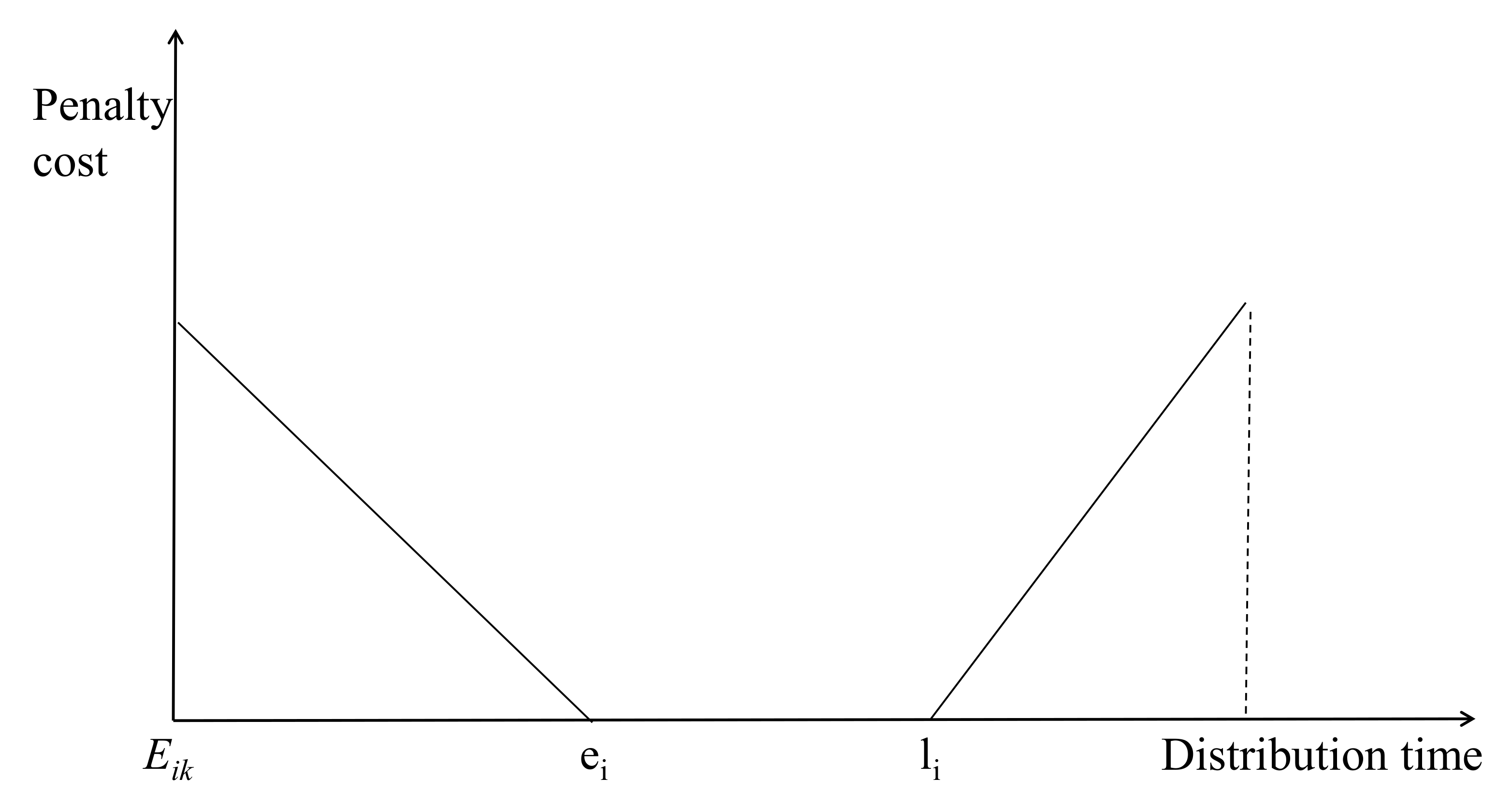
- Early arrival.
- 2.
- On-time arrival.
- 3.
- Delayed arrival.
- f3 indicates the waiting cost incurred per unit of time in case of early arrival.
- f4 denotes the delayed cost incurred per unit time when arriving late.
- Xik is a 0, 1 variable indicating that the kth vehicle performs the delivery operation for customer i.
5.4. Analysis of Customer Satisfaction
5.4.1. Fuzzy Appointment Time
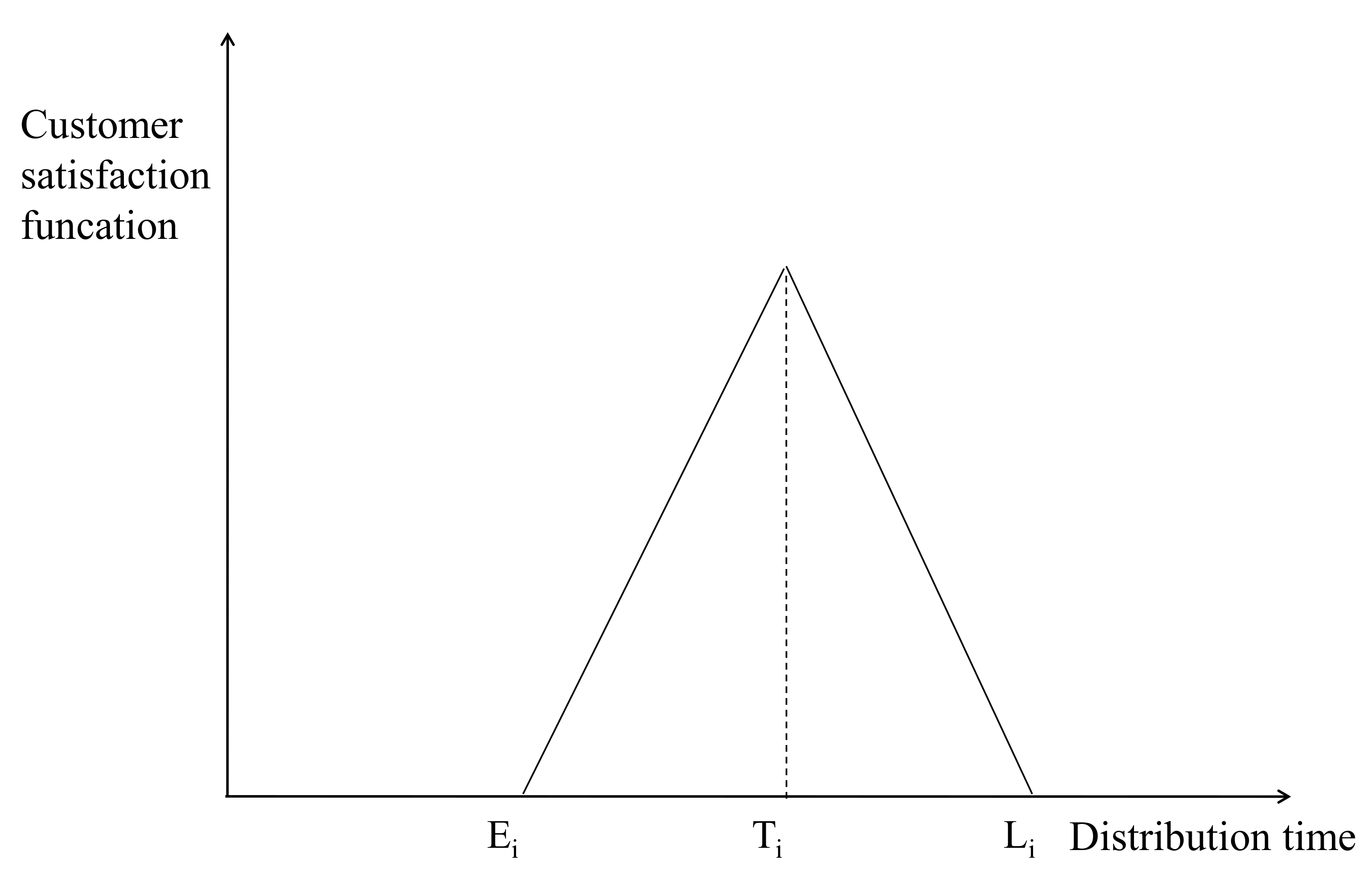
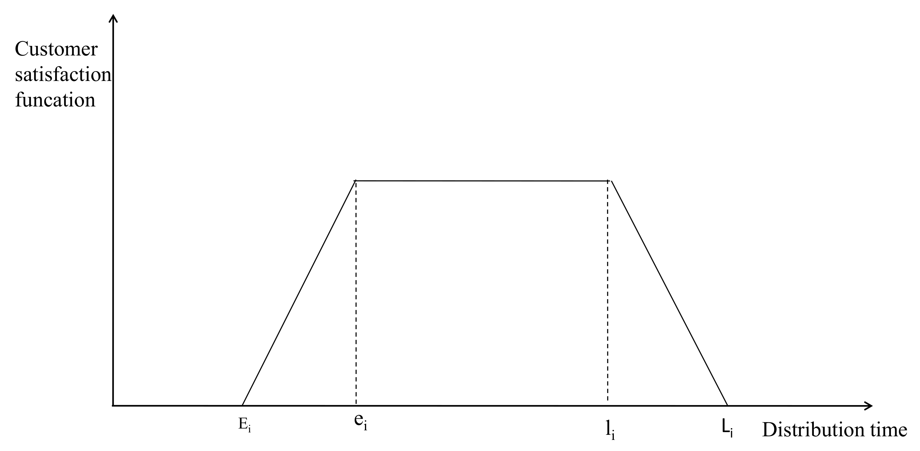
- When the delivery service occurs at the reservation time point Ti or within the time [ei, li], the customer expectation is met, and the satisfaction level reaches the highest.
- When the delivery service does not occur at the reservation time point Ti or within the time [ei, li] but is within the tolerable delivery time window [Ei, Li], the customer’s expectations are not achieved. However, the customer still chooses to accept the service. At this time, customer satisfaction is average.
- When the delivery service occurs outside the tolerable delivery window [Ei, Li], it is far from meeting the customer’s expectations, and customer satisfaction is the lowest.
5.4.2. Time Window-Based Customer Satisfaction Measurement
5.5. Model Building
5.5.1. Objective Function
- Treatment of multi-objective function
- 2.
- Final objective function
5.5.2. Constraints
- 0-1 variables
- 2.
- The actual weight of the vehicle shall not exceed the maximum weight of the vehicle.
- 3.
- Each customer has only one vehicle to deliver for him/her.
- 4.
- After a delivery task is completed, the delivery vehicle must go to the next delivery point.
- 5.
- The vehicle returns to the distribution center after completing all tasks.
- 6.
- The vehicle capacity fulfills the distribution needs of all customers.
- 7.
- The number of vehicles involved in distribution does not exceed the number of all distribution vehicles.
- 8.
- Meeting the time window constraints of all customers.
6. Case Study of Fresh Produce Distribution Center
6.1. Background Introduction
6.2. Data Collection and Processing
6.2.1. Constraints
6.2.2. Addresses and Codes of Distribution Points
6.2.3. Distribution Point Data Information
6.2.4. Demand Time Window
6.2.5. Other Parameters
6.3. Algorithm Parameter Setting
6.4. Model Solving
6.5. Comparative Analysis before and after Optimization
7. Conclusions and Prospects
7.1. Conclusions
- Due to the expansion of the distribution network of distribution centers, the previous method of judging distribution paths based on manual experience can no longer adapt to the growing fresh agricultural product distribution centers.
- R-FAPDC has its value. It has the typical characteristics of fresh trade distribution in coastal areas. Suppose the distribution problem research of such object considers the particular timeliness of fresh agricultural products distribution, constructs a multi-objective distribution path optimization model with time window constraints, and uses the genetic algorithm to derive a reasonable distribution route that meets the independent characteristics. In that case, it will be of great significance to improve the efficiency of trade distribution.
- The trade distribution path scheme optimized by the genetic algorithm can reduce the distribution cost of fresh agricultural products distribution centers and improve customer satisfaction.
- The genetic algorithm can bring economic benefits and reduce transportation losses in trade for the trade distribution centers with the same spatial characteristics and quality characteristics as R-FAPDC.
7.2. Data Collection and Processing
7.2.1. Emphasis on the Use of Genetic Algorithms in Planning Trade Distribution Path
7.2.2. Development of a Planning System of Trade Distribution Routes with High Adaptability
7.2.3. Strengthening the Rational Setting of Worker Performance in the Management of Organizational Operations
7.2.4. Establishing a High-Quality Logistics Service Standard System to Realize the Benign Development of Enterprise Distribution Work in the Process of Winning Customers
8. Deficiencies and Prospects
8.1. Deficiencies
- Some specific conditional restrictions are proposed in the model assumptions section. For example, all delivery vehicles are the same model, and the customer demand at the delivery point is always the same.
- In the data collection part, the customer demand information is mainly derived from the system records of R-FAPDC. This is a real-time data record. The distribution of data information may change at any time, which in turn affects the optimization effect. In this paper, the supply information of distribution nodes is known in advance. However, in reality, the supply quantities of distribution points are uncertain. This may lead to unforeseen new problems when implementing specific solutions.
- The optimized distribution path scheme is not implemented in practice in this paper due to the time constraints of the study and personal and professional levels. Therefore, the specific implementation effects in the distribution environment have not been studied in depth.
8.2. Prospects
- Subsequent research should continuously optimize the algorithm. This paper only uses the genetic algorithm for path optimization solutions. There are many path optimization algorithms. Each algorithm has its advantages and disadvantages. Solving such problems with a single algorithm will inevitably have drawbacks and defects. The next step can be to improve the genetic algorithm or combine the genetic algorithm with other heuristic algorithms.
- The distribution center should use modern intelligent technology to monitor the distribution process. In the future implementation of the distribution plan, consider in-depth research in supervising the distribution process and grasping the optimization effect. In particular, with the wide application of IoT (“Internet of Things”) technology, fresh agricultural product distribution centers should use modern intelligent methods to monitor the distribution process effectively.
- Researchers should consider the freshness of agricultural products in the optimization model constraints. The confirmation and measurement of the freshness of the agricultural products are not considered in the distribution process, and no detailed constraints are established. In the following research, it is necessary to further quantify and reflect the freshness of fresh agricultural products in the model to improve the optimization effect comprehensively.
- Researchers should continue to study the main reasons affecting the distribution efficiency in the distribution process, such as congestion or the distribution efficiency affected by the receiving and inspection link. If the delivery time is delayed by the receiving and inspection process, blind matching can be considered. Compare the cost of blind distribution with the previous distribution cost to choose a more reasonable distribution method.
Author Contributions
Funding
Institutional Review Board Statement
Informed Consent Statement
Data Availability Statement
Conflicts of Interest
References
- Dabbene, F.; Gay, P.; Sacco, N. Optimisation of fresh-food supply chains in uncertain environments, Part I: Background and methodology. Biosyst. Eng. 2008, 99, 348–359. [Google Scholar] [CrossRef]
- Xie, R.; Han, S.; Jiang, Y.; Peng, Z. Comparison and Optimization of Circulation Modes of Fresh Agricultural Products Based on System Dynamics—The Case of China. J. Serv. Sci. Manag. 2018, 11, 297–322. [Google Scholar] [CrossRef]
- Ying, J. Decision Optimization for Cold Chain Logistics of Fresh Agricultural Products under the Perspective of Cost-Benefit. Libr. J. 2019, 6, 1–17. [Google Scholar]
- Taghipour, A.; Khazaei, M.; Azar, A.; Ghatari, A.R.; Hajiaghaei-Keshteli, M.; Ramezani, M. Creating Shared Value and Strategic Corporate Social Responsibility through Outsourcing within Supply Chain Management. Sustainability 2022, 14, 1940. [Google Scholar] [CrossRef]
- Akbari-Kasgari, M.; Khademi-Zare, H.; Fakhrzad, M.B.; Hajiaghaei-Keshteli, M.; Honarvar, M. De-signing a resilient and sustainable closed-loop supply chain network in copper industry. Clean Technol. Environ. Policy 2022, 24, 1553–1580. [Google Scholar] [CrossRef]
- Kaviyani, C.M.; Ghodsypour, S.H.; Hajiaghaei, K.M. Impact of adopting quick response and agility on supply chain compe-tition with strategic customer behavior. Sci. Iran. 2022, 29, 387–411. [Google Scholar]
- Li, M.; He, L.; Yang, G.; Lian, Z. Profit-Sharing Contracts for Fresh Agricultural Products Supply Chain Considering Spatio-Temporal Costs. Sustainability 2022, 14, 2315. [Google Scholar] [CrossRef]
- Jiang, Y.; Chen, L.; Fang, Y. Integrated Harvest and Distribution Scheduling with Time Windows of Perishable Agri-Products in One-Belt and One-Road Context. Sustainability 2018, 10, 1570. [Google Scholar] [CrossRef]
- Song, B.D.; Ko, Y.D. A vehicle routing problem of both refrigerated- and general-type vehicles for perishable food products delivery. J. Food Eng. 2016, 169, 61–71. [Google Scholar] [CrossRef]
- Banerjee, S.; Agrawal, S. Inventory model for deteriorating items with freshness and price dependent demand: Optimal discounting and ordering policies. Appl. Math. Model. 2017, 52, 53–64. [Google Scholar] [CrossRef]
- Yan, B.; Fan, J.; Wu, J.-W. Channel choice and coordination of fresh agricultural product supply chain. RAIRO—Oper. Res. 2021, 55, 679–699. [Google Scholar] [CrossRef]
- Hop, V.N.; Phan, P.P. Adaptive inertia weight particle swarm optimisation for a multi-objective capacitated vehicle routing problem with time window in air freight forwarding. Int. J. Syst. Manag. 2021, 40, 423–442. [Google Scholar]
- Oesterle, J.; Bauernhansl, T. Exact Method for the Vehicle Routing Problem with Mixed Linehaul and Backhaul Customers, Heterogeneous Fleet, time Window and Manufacturing Capacity. Procedia CIRP 2016, 41, 573–578. [Google Scholar] [CrossRef]
- Archetti, C.; Bianchessi, N.; Grazia, S.M. A branch-price-and-cut algorithm for the commodity constrained split delivery ve-hicle routing problem. Comput. Oper. Res. 2015, 64, 1–10. [Google Scholar] [CrossRef]
- Dimitrakos, T.; Kyriakidis, E. A single vehicle routing problem with pickups and deliveries, continuous random demands and predefined customer order. Eur. J. Oper. Res. 2015, 244, 990–993. [Google Scholar] [CrossRef]
- Annelieke, C.B.; Said, D.B.; Wout, E.H.; Dullaert, D.V. The Vehicle Routing Problem with Partial Outsourcing. Transport. Sci. 2020, 54, 855–1152. [Google Scholar]
- El Sayed, M.; Farahat, F.; Elsisy, M. A novel interactive approach for solving uncertain bi-level multi-objective supply chain model. Comput. Ind. Eng. 2022, 169, 108225. [Google Scholar] [CrossRef]
- Elsisy, M.A.; Elsaadany, A.S.; El Sayed, M.A. Using Interval Operations in the Hungarian Method to Solve the Fuzzy Assignment Problem and Its Application in the Rehabilitation Problem of Valuable Buildings in Egypt. Complexity 2020, 2020, 1–11. [Google Scholar] [CrossRef]
- Sadri, E.; Harsej, F.; Hajiaghaei-Keshteli, M.; Siyahbalaii, J. Evaluation of the components of intelligence and greenness in Iranian ports based on network data envelopment analysis (DEA) approach. J. Model. Manag. 2022, 17, 1008–1027. [Google Scholar] [CrossRef]
- El Sayed, M.A.; Ibrahim, A.B.; Pitam, S. A modified TOPSIS approach for solving stochastic fuzzy multi-level multi-objective fractional decision-making problem. Opsearch 2020, 57, 1374–1403. [Google Scholar] [CrossRef]
- El Sayed, M.A.; Abo, S.M.A. A novel approach for fully intuitionistic fuzzy multi-objective fractional transportation problem. Alex. Eng. J. 2021, 60, 1447–1463. [Google Scholar] [CrossRef]
- Elsisy, M.A.; El Sayed, M.A.; Abo, E.Y. A novel algorithm for generating Pareto frontier of bi-level multi-objective rough non-linear programming problem. Ain Shams Eng. J. 2021, 12, 2125–2133. [Google Scholar] [CrossRef]
- Juan, D.C.; Yoshinori, S. Vehicle Routing with Shipment Consolidation. Int. J. Prod. Econ. 2020, 227, 167–181. [Google Scholar]
- Ning, T.; An, L.; Duan, X. Optimization of cold chain distribution path of fresh agricultural products under carbon tax mechanism: A case study in China. J. Intell. Fuzzy Syst. 2021, 40, 10549–10558. [Google Scholar] [CrossRef]
- Huang, R.; Ning, J.; Mei, Z.; Fang, X.; Yi, X.; Gao, Y.; Hui, G. Study of delivery path optimization solution based on improved ant colony model. Multimed. Tools Appl. 2021, 80, 28975–28987. [Google Scholar] [CrossRef]
- Jia, X. Research on the Optimization of Cold Chain Logistics Distribution Path of Agricultural Products E-Commerce in Urban Ecosystem from the Perspective of Carbon Neutrality. Front. Ecol. Evol. 2022, 10, 966111. [Google Scholar] [CrossRef]
- Liu, X.; Peng, X.; Gu, G. Logistics Distribution Route Optimization Based on Genetic Algorithm. Comput. Intell. Neurosci. 2022, 2022, 8468438. [Google Scholar] [CrossRef]
- Zhang, W.Q.; Li, H.R.; Yang, W.D.; Zhang, G.H.; Gen, M. Hybrid multiobjective evolutionary algorithm considering combi-nation timing for multi-type vehicle routing problem with time windows. Comput. Ind. Eng. 2022, 171, 108435. [Google Scholar] [CrossRef]
- He, D. Intelligent Selection Algorithm of Optimal Logistics Distribution Path Based on Supply Chain Technology. Comput. Intell. Neurosci. 2022, 2022, 9955726. [Google Scholar] [CrossRef]
- Daneshdoost, F.; Hajiaghaei, K.M.; Sahin, R.; Niroomand, S. Tabu Search Based Hybrid Meta-Heuristic Approaches for Schedule-Based Production Cost Minimization Problem for the Case of Cable Manufacturing Systems. Informatica 2022, 33, 499–522. [Google Scholar] [CrossRef]
- Zheng, C.; Sun, K.; Gu, Y.; Shen, J.; Du, M. Multimodal Transport Path Selection of Cold Chain Logistics Based on Improved Particle Swarm Optimization Algorithm. J. Adv. Transp. 2022, 2022, 5458760. [Google Scholar] [CrossRef]
- Fan, Q.; Nie, X.X.; Yu, K.; Zuo, X.L. Optimization of Logistics Distribution Route Based on the Save Mileage Method and the Ant Colony Algorithm. Appl. Mech. Mater. 2013, 448–453, 3683–3687. [Google Scholar] [CrossRef]
- Sun, R.; Liu, M.; Zhao, L. Research on logistics distribution path optimization based on PSO and IoT. Int. J. Wavelets Multiresolution Inf. Process. 2019, 17, 1950051. [Google Scholar] [CrossRef]
- Zhai, R. Solving the Optimization of Physical Distribution Routing Problem with Hybrid Genetic Algorithm. J. Phys. Conf. Ser. 2020, 1550, 022001. [Google Scholar] [CrossRef]
- Wu, D.Q.; Wu, C.X. TDGVRPSTW of Fresh Agricultural Products Distribution: Considering Both Economic Cost and Environmental Cost. Appl. Sci. 2021, 11, 10579. [Google Scholar] [CrossRef]
- Zhang, B. The Optimization of Distribution Path of Fresh Cold Chain Logistics Based on Genetic Algorithm. Comput. Intell. Neurosci. 2022, 2022, 4667010. [Google Scholar] [CrossRef]
- Wang, X.; Cao, W. Research on optimization of distribution route for cold chain logistics cooperative distribution of fresh e-commerce based on price discount. J. Phys. Conf. Ser. 2021, 1732, 012041. [Google Scholar] [CrossRef]
- Zhao, Z.; Li, X.; Zhou, X. Distribution Route Optimization for Electric Vehicles in Urban Cold Chain Logistics for Fresh Products under Time-Varying Traffic Conditions. Math. Probl. Eng. 2020, 2020, 9864935. [Google Scholar] [CrossRef]
- Wu, F. Contactless Distribution Path Optimization Based on Improved Ant Colony Algorithm. Math. Probl. Eng. 2021, 2021, 5517778. [Google Scholar] [CrossRef]
- Wang, Z.; Wen, P. Optimization of a Low-Carbon Two-Echelon Heterogeneous-Fleet Vehicle Routing for Cold Chain Logistics under Mixed Time Window. Sustainability 2020, 12, 1967. [Google Scholar] [CrossRef]
- Xia, Y.K.; Fu, Z. Improved tabu search algorithm for the open vehicle routing problem with soft time windows and satis-faction rate. Clust. Comput. 2019, 22, 8725–8733. [Google Scholar] [CrossRef]
- Liu, H. Optimization of Dairy Distribution Path Based on Genetic Algorithm. J. Phys. Conf. Ser. 2019, 1345, 042054. [Google Scholar] [CrossRef]
- Olaniyi, O.S.; James, A.K. On the Application of a Modified Genetic Algorithm for Solving Vehicle Routing Problems with Time Windows and Split Delivery. IAENG Int. J. Appl. Math. 2022, 52, 1–9. [Google Scholar]
- Zhang, Y.; Jiang, T.; Sun, J.; Fu, Z.; Yu, Y. Sustainable Development of Urbanization: From the Perspective of Social Security and Social Attitude for Migration. Sustainability 2022, 14, 10777. [Google Scholar] [CrossRef]
- Dou, S.; Liu, G.; Yang, Y. A New Hybrid Algorithm for Cold Chain Logistics Distribution Center Location Problem. IEEE Access 2020, 8, 88769–88776. [Google Scholar] [CrossRef]


| Classification Standards | Type | Definition |
|---|---|---|
| Type of vehicle | Single-type distribution | Delivery by one vehicle type |
| Multi-type distribution | Delivery by multiple vehicle types | |
| Number of distribution centers | Vehicle routing with a single depot | One distribution center |
| Vehicle routing with multiple depots | Multiple distribution centers | |
| Number of optimization targets | Single target | One optimization target |
| Multiple targets | Multiple optimization targets | |
| Time windows | Hard time windows | Delivery within the time window |
| Soft time windows | Deliveries can be made outside the time window, but with penalties. | |
| No time windows | No limitation on delivery time | |
| Fuzzy time windows | Setting a time window that can influence customer satisfaction | |
| Return Restrictions | Open vehicle routing | Vehicles do not need to return to the distribution center. |
| Enclosed vehicle routing | Vehicles need to be returned to the distribution center. | |
| Whether the decision information is certain | Static | Information on distribution environment and demand point conditions is certain. |
| Dynamic | Information on distribution environment and demand point conditions is uncertain. | |
| Vehicle loading | Fully loaded | The load of the vehicle is less than the single demand point requirement. |
| Non-full load | The load of the vehicle is greater than the single demand point needs. |
| Symbols | Practical Meanings | Symbols | Practical Meanings |
|---|---|---|---|
| n | The number of vehicles put into the distribution chain. | [ei,li] | Customer i specified deliverable time period. |
| k | The kth vehicle.k∈{1,2,⋯,n} | Ei | The earliest delivery time tolerated by customer i. |
| i, j, p | Distribution center or customer location. | Li | The latest delivery time that can be tolerated by customer i. |
| R | R = {i, j, p|i, j, p = 1,⋯,m} | [Ei,Li] | The delivery time period that can be tolerated by customer i. |
| f1 | Fixed costs incurred per vehicle in the distribution chain. | Ti | Customer i defined time point for satisfactory service. |
| Dij | Miles traveled between customer i and j. | Aik | Actual time of arrival of the kth vehicle at customer i’s location |
| f2 | Transportation cost per unit distance | f3 | Waiting costs incurred per unit of time in case of early arrival |
| Xijk | 0,1 variables, indicating that the kth vehicle completes the delivery operation for customer i,j. | f4 | Delayed costs incurred per unit of time in case of delayed arrival |
| Eik | Earliest time for the kth vehicle to arrive at customer i’s location | Xik | 0,1 variables, indicating that the delivery operation of customer i is completed by the kth vehicle |
| Lik | Latest time for the kth vehicle to arrive at customer i’s location | Qk | Actual load of the kth vehicle |
| [Eik,Lik] | Time period for the arrival of the kth vehicle at customer i’s location | qi | Actual demand of customer i |
| ei | The earliest time that can be delivered as specified by customer i | Q | Maximum load of distribution vehicles |
| li | The latest deliverable time specified by customer i |
| Name | Address | Code |
|---|---|---|
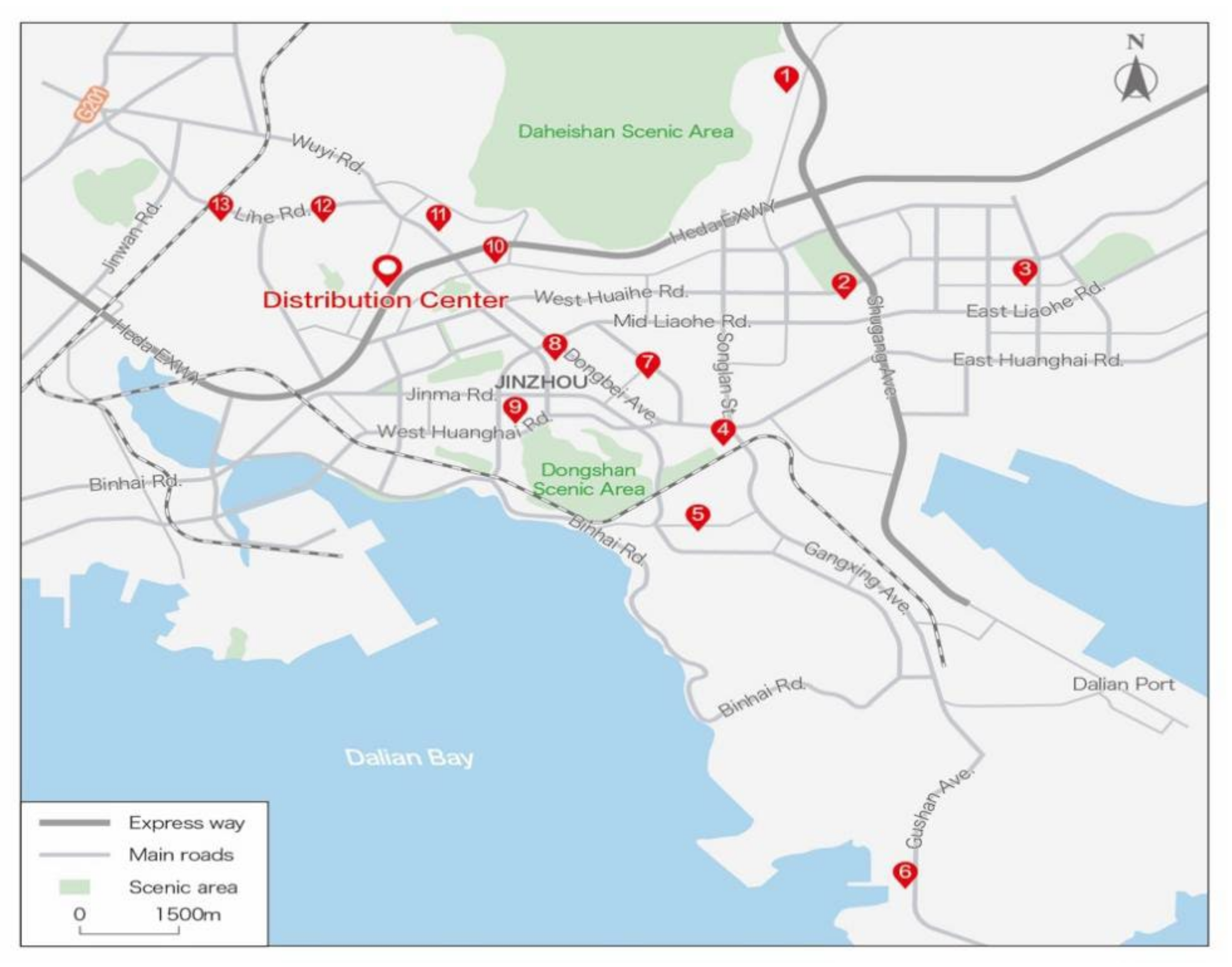
| R Fresh produce distribution center | No. 1, Yingjun Road, Jinzhou District, Dalian | 0—distribution center |
| Distribution point 1 | No. 10 Xuefu Street, Jinzhou District, Dalian | 1—P1 |
| Distribution point 2 | Huaihe Middle Road, Jinzhou District, Dalian | 2—P2 |
| Distribution point 3 | East Liahe Road and Shuang D1 Street, Jinzhou District, Dalian | 3—P3 |
| Distribution point 4 | Intersection of Dong’an Road and Donghui Street, Jinzhou District, Dalian | 4—P4 |
| Distribution point 5 | No. 50–66, Pengyun Home, Jinzhou District, Dalian | 5—P5 |
| Distribution point 6 | Near Kushan Middle Road, Jinzhou District, Dalian | 6—P6 |
| Distribution point 7 | Near Maqiaozi Street, Jinzhou District, Dalian | 7—P7 |
| Distribution point 8 | No. 19, Tonghui Road, Jinzhou District, Dalian | 8—P8 |
| Distribution point 9 | No. 18, West Liahe Road, Jinzhou District, Dalian | 9—P9 |
| Distribution point 10 | No. 31 Tieshan West Road, Jinzhou District, Dalian | 10—P10 |
| Distribution point 11 | No. 14 Tieshan West Road, Jinzhou District, Dalian | 11—P11 |
| Distribution point 12 | No. 288 Jingang Road, Jinzhou District, Dalian | 12—P12 |
| Distribution point 13 | Intersection of Jingang Road and Longwan Road, Jinzhou District, Dalian | 13—P13 |
| Node Coordinates | Horizontal Coordinate (Latitude) | Vertical Coordinate (Longitude) | Distance (km) | Demand (t) |
|---|---|---|---|---|
| 1 | 39.106662 | 121.826772 | 10.3 | 0.43 |
| 2 | 39.077017 | 121.856698 | 7.8 | 0.55 |
| 3 | 39.070833 | 121.871083 | 11.5 | 0.26 |
| 4 | 39.046255 | 121.818441 | 7.0 | 0.5 |
| 5 | 39.031466 | 121.813384 | 7.9 | 0.47 |
| 6 | 38.969756 | 121.852591 | 17.5 | 0.70 |
| 7 | 39.054987 | 121.808604 | 5.8 | 0.485 |
| 8 | 39.104574 | 121.840646 | 10.9 | 0.37 |
| 9 | 39.051454 | 121.781714 | 3.7 | 0.44 |
| 10 | 39.075549 | 121.775135 | 2.5 | 0.5 |
| 11 | 39.071659 | 121.765949 | 3.0 | 0.55 |
| 12 | 39.083375 | 121.747865 | 4.2 | 0.45 |
| 13 | 39.082096 | 121.730709 | 4.0 | 0.44 |
| Node Label (km) | 1 | 2 | 3 | 4 | 5 | 6 | 7 | 8 | 9 | 10 | 11 | 12 | 13 |
|---|---|---|---|---|---|---|---|---|---|---|---|---|---|
| 1 | 0 | ||||||||||||
| 2 | 5.1 | 0 | |||||||||||
| 3 | 8.6 | 4.8 | 0 | ||||||||||
| 4 | 7.8 | 5.4 | 8.2 | 0 | |||||||||
| 5 | 9.7 | 7.3 | 10.1 | 3.2 | 0 | ||||||||
| 6 | 17.8 | 15.4 | 15.7 | 11.4 | 10.1 | 0 | |||||||
| 7 | 7.8 | 5.4 | 8.2 | 2.6 | 5.1 | 13.2 | 0 | ||||||
| 8 | 7.0 | 4.6 | 5.5 | 9.0 | 11.1 | 19.3 | 8.4 | 0 | |||||
| 9 | 10.5 | 7.7 | 10.4 | 3.8 | 5.1 | 14.4 | 8.7 | 10.7 | 0 | ||||
| 10 | 7.1 | 7.2 | 9.9 | 5.4 | 7.8 | 16 | 3.4 | 8.2 | 4.5 | 0 | |||
| 11 | 8.3 | 7.7 | 10.5 | 5.9 | 8.4 | 16.5 | 4.4 | 9.4 | 5.0 | 1.0 | 0 | ||
| 12 | 10.5 | 10.0 | 12.7 | 8.2 | 10.6 | 18.8 | 6.6 | 16.1 | 7.3 | 3.2 | 2.2 | 0 | |
| 13 | 12.1 | 11.6 | 14.3 | 9.8 | 11.0 | 20.4 | 8.2 | 13.2 | 7.5 | 4.8 | 3.8 | 1.7 | 0 |
| Node Coordinates | Optimal Service Time Window [ei,li] | Tolerable Time Window [Ei,Li] | ||
|---|---|---|---|---|
| Earliest Time ei | Latest Time li | Earliest Time Ei | Latest Time Li | |
| 1 | 06.00 | 09.00 | 05.00 | 10.00 |
| 2 | 06.00 | 09.00 | 05.00 | 10.00 |
| 3 | 05.30 | 08.30 | 04.30 | 09.30 |
| 4 | 06.30 | 09.30 | 05.30 | 10.30 |
| 5 | 05.30 | 08.30 | 04.30 | 09.30 |
| 6 | 06.30 | 09.30 | 05.30 | 10.30 |
| 7 | 06.00 | 09.00 | 05.00 | 10.00 |
| 8 | 06.30 | 09.30 | 05.30 | 10.30 |
| 9 | 07.00 | 10.00 | 06.00 | 11.00 |
| 10 | 05.30 | 08.30 | 04.30 | 09.30 |
| 11 | 06.30 | 09.30 | 05.30 | 10.30 |
| 12 | 06.00 | 09.00 | 05.00 | 10.00 |
| 13 | 05.30 | 08.30 | 04.30 | 09.30 |
| Parameter | Takes Values |
|---|---|
| Unit vehicle fixed cost (CNY/vehicle) | 150.0 |
| Unit distance transportation cost (CNY/km) | 2.0 |
| Early arrival waiting fee (CNY/h) | 10.0 |
| Delayed arrival delay fee (CNY/h) | 20.0 |
| Vehicle maximum load capacity (t) | 1.5 |
| Average vehicle speed (km/h) | 30.0 |
| Average customer service time (h) | 0.5 |
| Parameter | Initial Population Size | Crossover Probability | Mutation Probability | Maximum Number of Iterations |
|---|---|---|---|---|
| Takes values | 200 | 0.9 | 0.1 | 200 |
| Route Number | Driving Path |
|---|---|
| 1 | 0-2-8-1-0 |
| 2 | 0-11-10-0 |
| 3 | 0-3-6-5-0 |
| 4 | 0-7-4-9-0 |
| 5 | 0-13-12-0 |
| Route Number | Driving Path |
|---|---|
| 1 | 0-10-1-0 |
| 2 | 0-3-2-0 |
| 3 | 0-7-8-0 |
| 4 | 0-4-9-0 |
| 5 | 0-5-6-0 |
| 6 | 0-11-12-13-0 |
| Vehicle Number | Order of Visit | Load Capacity (t) | Route (km) | Time (h) | Full Load Rate (%) |
|---|---|---|---|---|---|
| 1 | 0-10-1-0 | 0.93 | 19.9 | 1.66 | 62 |
| 2 | 0-3-2-0 | 0.81 | 24.1 | 1.80 | 54 |
| 3 | 0-7-8-0 | 0.85 | 25.1 | 1.84 | 57 |
| 4 | 0-4-9-0 | 0.94 | 8.2 | 1.27 | 63 |
| 5 | 0-5-6-0 | 1.17 | 35.5 | 2.18 | 78 |
| 6 | 0-11-12-13-0 | 1.44 | 10.9 | 1.86 | 96 |
| Route Number | Time Nodes |
|---|---|
| 1 | 0(05:00)-10(05:05–05:35)-1(05:50–06:20)-0(06:40) |
| 2 | 0(05:00)-3(05:23–05:53)-2(06:03–06:33)-0(06:49) |
| 3 | 0(05:00)-7(05:12–05:42)-8(05:59–06:29)-0(06:51) |
| 4 | 0(05:00)-4(05:14–05:44)-9(05:52–06:22)-0(07:00) |
| 5 | 0(05:00)-5(05:17–05:47)-6(06:07–06:37)-0(07:12) |
| 6 | 0(05:00)-11(05:06–05:36)-12(05:41–06:11)-13(06:15–06:45)-0(06:53) |
| Vehicle Number | Fixed Cost (CNY) | Transportation Cost (CNY) | Penalty Cost (CNY) | Total |
|---|---|---|---|---|
| 1 | 150 | 39.8 | 20 | 209.8 |
| 2 | 150 | 48.2 | 10 | 208.2 |
| 3 | 150 | 50.2 | 20 | 220.2 |
| 4 | 150 | 16.4 | 40 | 206.4 |
| 5 | 150 | 71.0 | 20 | 241.0 |
| 6 | 150 | 21.8 | 40 | 211.8 |
| Vehicle Number | Order of Visit | Load Capacity (t) | Route (km) | Time (h) | Full Load Rate (%) |
|---|---|---|---|---|---|
| 1 | 0-2-8-1-0 | 1.35 | 29.7 | 2.49 | 90 |
| 2 | 0-11-10-0 | 1.05 | 6.5 | 1.22 | 70 |
| 3 | 0-3-6-5-0 | 1.43 | 45.2 | 3.00 | 95 |
| 4 | 0-7-4-9-0 | 1.42 | 15.9 | 2.03 | 95 |
| 5 | 0-13-12-0 | 0.89 | 9.9 | 1.33 | 60 |
| Route Number | Time Nodes |
|---|---|
| 1 | 0(05:00)-2(05:16–05:46)-8(05:56–06:26)-1(06:40–07:10)-0(07:30) |
| 2 | 0(05:00)-11(05:06–05:36)-10(05:38–06:08)-0(06:13) |
| 3 | 0(05:00)-3(05:23–05:53)-6(06:25–06:55)-5(06:15–06:45)-0(07:00) |
| 4 | 0(05:00)-7(05:20–05:50)-4(05:56–06:26)-9(06:34–07:04)-0(07:12) |
| 5 | 0(05:00)-13(05:08–05:38)-12(05:42–06:12)-0(06:20) |
| Vehicle Number | Fixed Cost (CNY) | Transportation Cost (CNY) | Penalty Cost (CNY) | Total |
|---|---|---|---|---|
| 1 | 150 | 59.4 | 20 | 229.4 |
| 2 | 150 | 13.0 | 20 | 183.0 |
| 3 | 150 | 90.4 | 20 | 260.4 |
| 4 | 150 | 31.8 | 30 | 211.8 |
| 5 | 150 | 19.8 | 20 | 189.8 |
| Before Optimization | After Optimization | Comparison before and after Optimization | |
|---|---|---|---|
| Number of vehicles (vehicles) | 6.0 | 5.0 | −1.0 |
| Fixed cost (CNY) | 900.0 | 750.0 | −150.0 |
| Transportation cost (CNY) | 247.4 | 214.4 | −33.0 |
| Penalty cost (CNY) | 150.0 | 110.0 | −40.0 |
| Distribution cost (CNY) | 1294.4 | 1074.4 | −220.0 |
| Distribution mileage (km) | 123.7 | 107.2 | −16.5 |
| Customer satisfaction (%) | 87.9 | 88.3 | +0.4 |
Publisher’s Note: MDPI stays neutral with regard to jurisdictional claims in published maps and institutional affiliations. |
© 2022 by the authors. Licensee MDPI, Basel, Switzerland. This article is an open access article distributed under the terms and conditions of the Creative Commons Attribution (CC BY) license (https://creativecommons.org/licenses/by/4.0/).
Share and Cite
Sun, J.; Jiang, T.; Song, Y.; Guo, H.; Zhang, Y. Research on the Optimization of Fresh Agricultural Products Trade Distribution Path Based on Genetic Algorithm. Agriculture 2022, 12, 1669. https://doi.org/10.3390/agriculture12101669
Sun J, Jiang T, Song Y, Guo H, Zhang Y. Research on the Optimization of Fresh Agricultural Products Trade Distribution Path Based on Genetic Algorithm. Agriculture. 2022; 12(10):1669. https://doi.org/10.3390/agriculture12101669
Chicago/Turabian StyleSun, Jun, Tianhang Jiang, Yufei Song, Hao Guo, and Yushi Zhang. 2022. "Research on the Optimization of Fresh Agricultural Products Trade Distribution Path Based on Genetic Algorithm" Agriculture 12, no. 10: 1669. https://doi.org/10.3390/agriculture12101669
APA StyleSun, J., Jiang, T., Song, Y., Guo, H., & Zhang, Y. (2022). Research on the Optimization of Fresh Agricultural Products Trade Distribution Path Based on Genetic Algorithm. Agriculture, 12(10), 1669. https://doi.org/10.3390/agriculture12101669


