Article

Future Scenarios for Viticultural Suitability under Conditions of Global Climate Change in Extremadura, Southwestern Spain

by
Francisco J. Moral
1,*,
Cristina Aguirado
1,
Virginia Alberdi
1,
Abelardo García-Martín
2,
Luis L. Paniagua
2 and
Francisco J. Rebollo
3
1
Departamento de Expresión Gráfica, Escuela de Ingenierías Industriales, Universidad de Extremadura, Avda. de Elvas, s/n, 06006 Badajoz, Spain
2
Departamento de Ingeniería del Medio Agronómico y Forestal, Escuela de Ingenierías Agrarias, Universidad de Extremadura, Avda. Adolfo Suárez, s/n, 06007 Badajoz, Spain
3
Departamento de Expresión Gráfica, Escuela de Ingenierías Agrarias, Universidad de Extremadura, Avda. Adolfo Suárez, s/n, 06007 Badajoz, Spain
*
Author to whom correspondence should be addressed.
Agriculture 2022, 12(11), 1865; https://doi.org/10.3390/agriculture12111865
Submission received: 30 September 2022 / Revised: 2 November 2022 / Accepted: 4 November 2022 / Published: 6 November 2022
(This article belongs to the Section Ecosystem, Environment and Climate Change in Agriculture)

Abstract

:
Weather condition is the main factor affecting winegrape production. Therefore, it is necessary to study the expected consequences of climate change on vineyards to anticipate adaptation strategies. To analyse how viticulture in Extremadura, in southwestern Spain, could be affected by warming, four temperature-based indices describing the suitability for grape production were computed for a reference period (1971–2005) and three future periods (2006–2035, 2036–2065, and 2066–2095). Projections were computed using a set of 10 global climate model (GCM) and regional climate model (RCM) combinations under two representative concentration pathways (RCP) scenarios, RCP 4.5, and RCP 8.5. Results showed that most of the Extremaduran region will remain suitable for winegrape production during the period 2006–2035. Later, for the mid-century, 2036–2065, depending on the considered index and the scenario, between 65% and 92% of the total area of Extremadura will be too hot for viticulture; for the end of the century, 2066–2095, between 80% and 98% of the region will be too hot. However, under the RCP 4.5 scenario, a few zones could be suitable for winegrape production but will require the use of new varieties and techniques to resist heat and drought stress.

1. Introduction

Meteorological changes from one year to the next often affect the optimal environmental conditions for crop development, altering crop characteristics such as fruit growth periods, ripening characteristics, and composition [1,2]. Accordingly, vineyard productivity and sustainability primarily respond to weather conditions and are, therefore, highly sensitive to climate change. Some previous studies have shown that grape yield and composition are affected by the rise in air temperature derived from climate change [3,4].
The impact of weather conditions, both current and projected, on viticulture has been studied in numerous wine-growing regions using different methods [5,6,7,8] and in different geographical areas, such as Europe [9,10], France [11], Serbia [12], Australia [13], and even worldwide [2,14], as well as in smaller areas, such as Rias Baixas, in Spain [15], the Douro valley, in Portugal [16], Emilia-Romagna, in Italy [17], and by Lake Neuchatel, in Switzerland [18]. All these studies have shown that climate strongly affects the spatial distribution of wine-growing regions, concluding that land use zoning is a basic tool for adequately understanding the suitability and sustainability of wine production.
The wine sector is crucial for Europe, which accounts for approximately 50% of the world’s vineyards [19]. On this continent—as well as globally—Spain has the largest area under vines, totalling 940,000 ha of the vineyard [20]. Wine production has strong social significance in many countries; therefore, several studies have investigated how global warming affects viticulture by performing climate projections, which are valuable tools for evaluating present and future scenarios in wine-growing areas [12,21,22].
Greenhouse gases, such as carbon dioxide, nitrous oxide, methane and halocarbons, and aerosols and their precursors emitted into the atmosphere by human activities are the main cause of global warming [23]. Thus, the future concentration of these gases in the atmosphere will define any climate projection. Four climate scenarios, called Representative Concentration Pathways (RCP) scenarios (RCP 2.6, RCP 4.5, RCP 6, and RCP 8.5), were presented by the Intergovernmental Panel of Climate Change (IPCC) in their Fifth Assessment Report [24]. The RCP scenarios consider the technological and economic development of society to estimate concentrations of radiative forcing agents and the temporal development of emissions, that is, greenhouse gases, aerosols, and their precursors. According to the RCP scenarios, the most relevant greenhouse gas, atmospheric CO2 concentration, could be between 420 and 940 ppm by the end of the 21st century [24,25], whereas currently, it is approximately 414 ppm. The combined effect of this increase with the expected increase of other greenhouse gases reinforced by natural feedback processes will suppose a 1–4 °C increase in mean global temperature relative to the period 1986–2005, depending on the RCP scenario [24].
Through the Coordinated Regional Downscaling Experiment (CORDEX) project, 65 sets of climate projections are generated by dynamically downscaling CMIP6 GCM (general circulation models) output using regional climate models (RCM) [26]. These GCMs-RCMs combinations simulate the climate system. Climate projections mainly depend on the future concentration of substances such as greenhouse gases (GHGs). This dependence relation is represented by using the four RCP scenarios mentioned above. The spatial resolution of the climate projections performed in the CORDEX project is 12.5 or 25 km. High spatial resolution is crucial for viticultural studies [27,28] because the regions where the vine is grown usually have a complex topography.
Numerous specific climatic indices, either general or related to this crop in some way, can be used to analyse the suitability of viticulture in a given area. Some of these indices are derived from temperature—for example, the average temperature during the vine growth period is commonly used. Other indices involving thermal integrals are also used to measure the sum of heat during this period [29].
Four temperature-derived indices are commonly used to measure the heat summation during the growing period. The Winkler index (WI) measures in degree-days the duration of the growing period, GDD [30]. Another similar index is the growing season temperature, GST [31]: it establishes the requirements of varieties to ripen (sugar accumulation in berries). Huglin [32] developed the heliothermal index, HI: it considers the average and maximum temperatures, weighting the accumulated temperatures to the daytime period to provide the heat summation. The biologically effective degree-day index, BEDD, considers the optimal growing interval for grapevine and a day length correction to calculate heat summation, adjusted for the diurnal temperature range [33]. Many studies have been conducted using these indices in different regions [5,34,35].
Extremadura has the second-largest grapevine-growing area in the Iberian Peninsula, with some wineries of international prestige. The climatic characteristics of this region related to viticulture have been accurately described by Moral et al. [29,35]. An important climatic spatial variability was found in the region, despite it being one of the hottest wine-producing regions worldwide.
The aforementioned studies conducted in Extremadura, Spain, addressed historical time periods. However, a spatial variability study based on bioclimatic indices using data derived from combining GCMs and RCMs for different scenarios would provide information on future climate changes that could affect vines in the Extremadura region.
Considering the above, this research aimed at studying high-resolution climate projections performed with a set of 10 GCM-RCM combinations for RCP 4.5 and RCP 8.5 scenarios in Extremadura and for various future periods until the end of the 21st century. Additionally, the spatial variations of each bioclimatic index in each time period were analysed to assess their implications for the future viticultural suitability of the region.

2. Materials and Methods
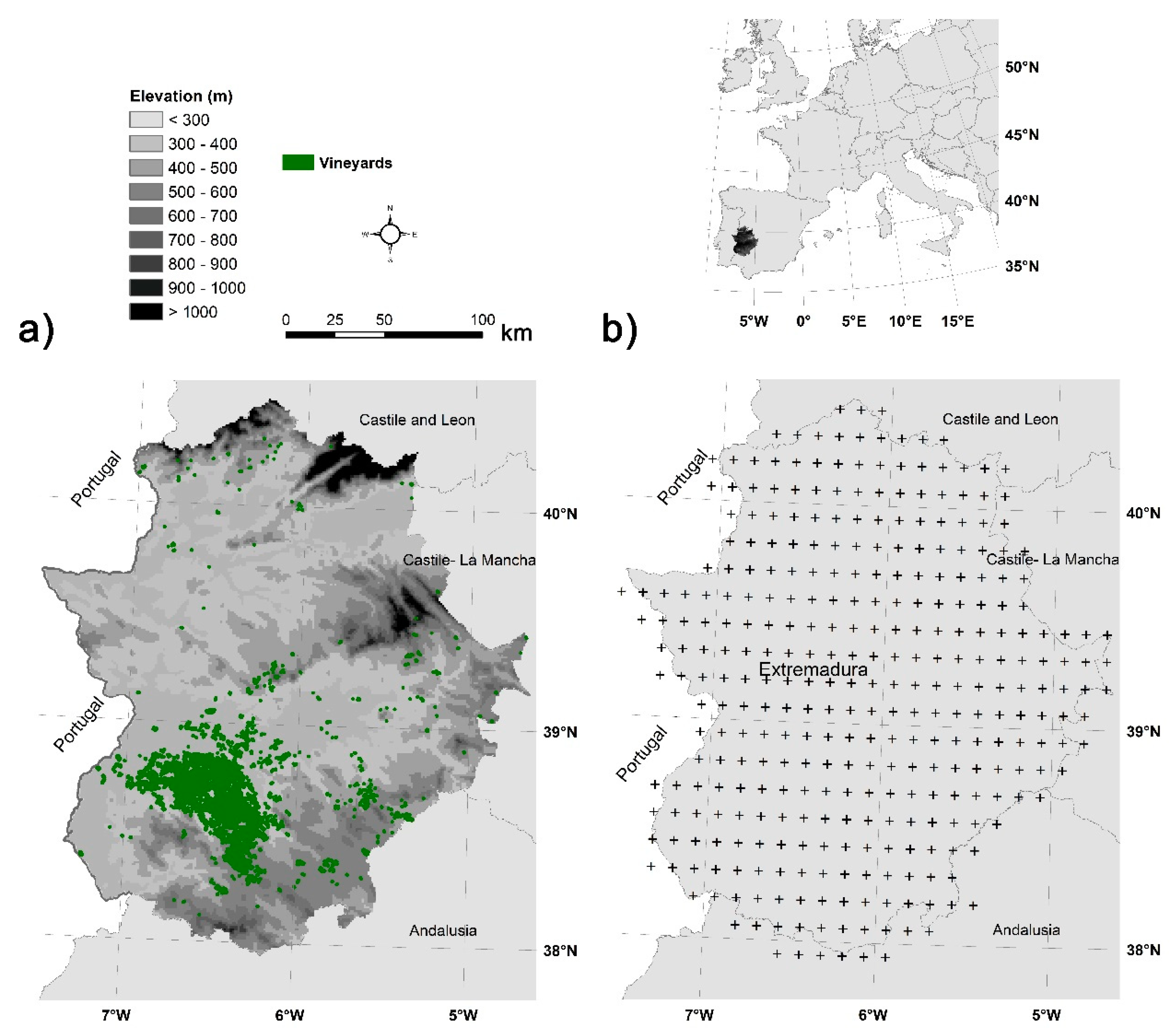
2.1. Study Area

This study was conducted in Extremadura. This region is located in Southwestern Spain, bordering Portugal (Figure 1), and spans across 41,634 km2, between 37°57′ and 40°29′ N latitude and 4°39′ and 7°33′ W longitude.
In Extremadura, the climate is mainly Mediterranean, with oceanic influences due to its proximity to the Atlantic Ocean. Precipitation shows a marked interannual variability, with a dry season from June to September and a rainy season from October to May, which accounts for 80% of the total precipitation. Droughts commonly occur in Extremadura every 8–9 years, lasting approximately two years [36]. In general, Extremadura is considered a semiarid region, where summers are very hot and dry, reaching temperatures above 40 °C; winters are either rainy and mild or cold and dry.
The average elevation in the region is 425 m above sea level (m a.s.l.), although the altitude ranges from 2091 m a.s.l. in Sierra de Gredos, to the north of the region, to 116 m a.s.l. in the Guadiana valley, in the centre of the region. The terrain varies considerably, with Sierra Morena, other mountains, and large grassland areas to the south, the vast Alcántara and Brozas plains, the San Pedro mountains, and the Guadiana valley to the west, the Tagus River and the steep Las Villuercas mountains to the east, and the Central System to the north, where the highest locations in the region are found, in addition to other lower mountain ranges (such as Sierra de Gata and Las Hurdes) with fertile valleys between them.
Extremadura has 83,763 ha of vineyards, accounting for 9.24% of Spanish vineyards, ranking second among Spanish autonomous communities, only behind Castilla y La Mancha [37]. Furthermore, it has the Ribera del Guadiana Protected Designation of Origin (PDO) along with two other Protected Geographical Indications (PGIs) for wine, namely Designation-of-origin Cava and Extremadura wine. Figure 1 shows the elevation map of the region with vineyard areas.

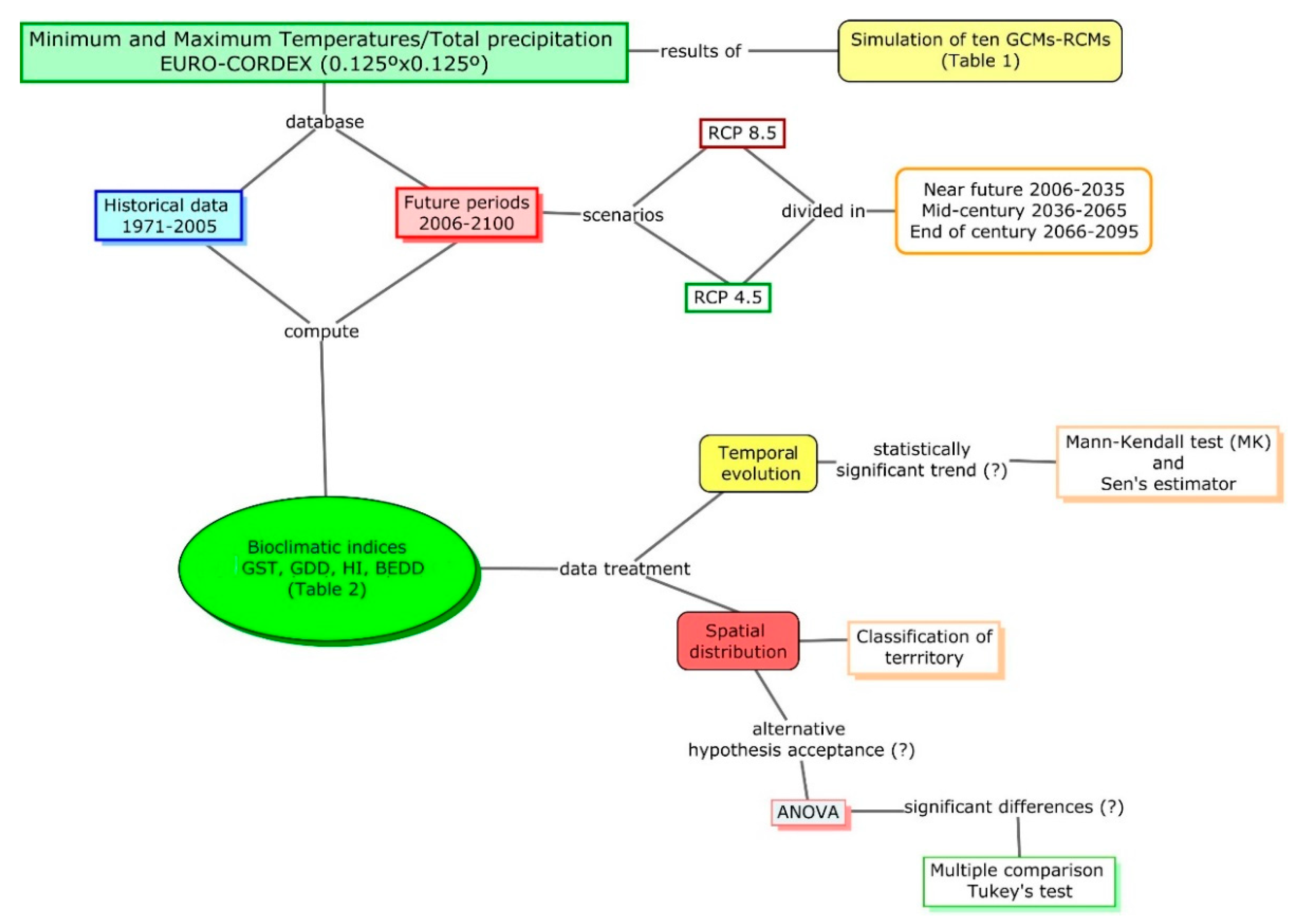
2.2. Climate Data and Future Scenarios

Daily maximum and minimum temperatures data were obtained from http://cordex.org/ (accessed on 25 June 2022) for the historical period 1971−2005 and two scenarios between 2006 and 2095 at 0.125° grid resolution (approximately 12.5 km). The bioclimatic indices considered in this study were computed at the same spatial resolution, using historical data and data from a set of 10 GCM-RCM combinations (Table 1) under both RCP 4.5 and RCP 8.5 for the future. The RCP 4.5 scenario corresponds to a stabilisation of the additional anthropogenic radiative forcing relative to the pre-industrial levels, without an overshoot pathway, at 4.5 W/m2 by the end of the 21st century. The RCP 8.5 corresponds to an increase in radiative forcing of 8.5 W/m2 by the end of the 21st century. All regional changes were analysed within the geographical sector comprising Extremadura, using data for four-time intervals: 1971–2005 (reference, P0), 2006–2035 (P1), 2036–2065 (P2) and 2066–2095 (P3). Grid points located in Extremadura, and a few others along its boundaries, where temperature and precipitation were estimated according to different scenarios, were considered to calculate the bioclimatic indices (Figure 1). The use of a few points along the boundaries of the region can benefit subsequent estimates in border areas.

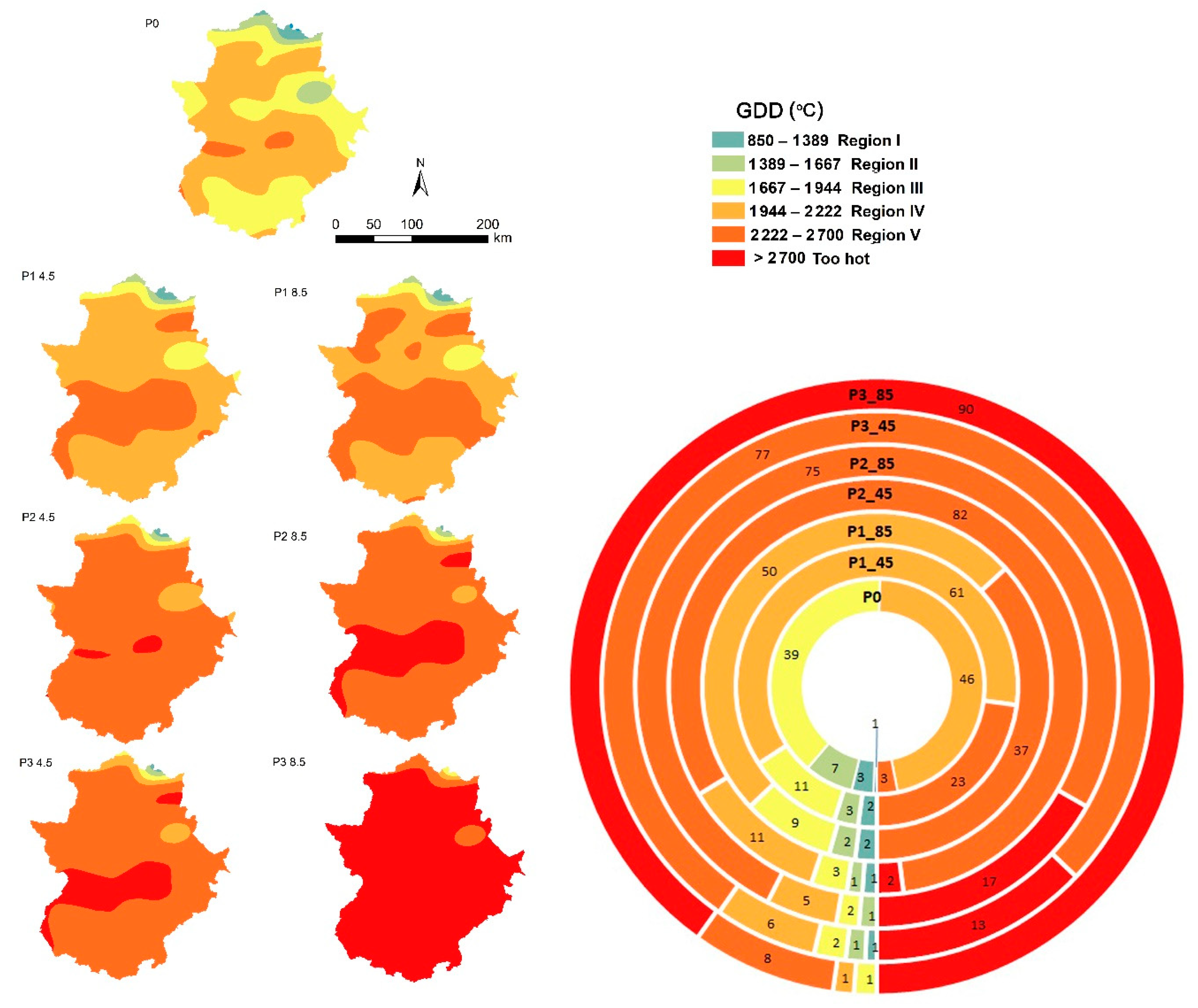
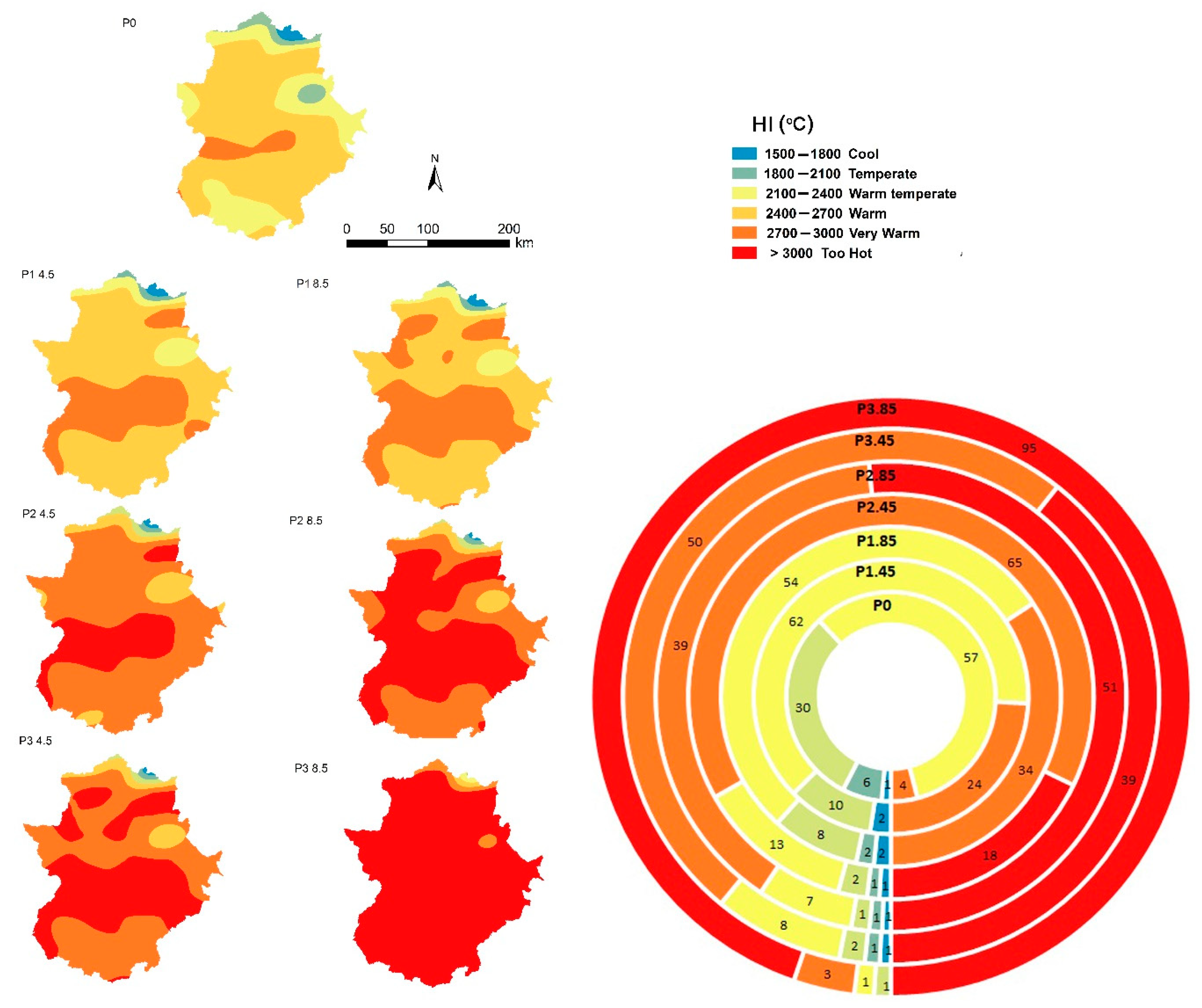
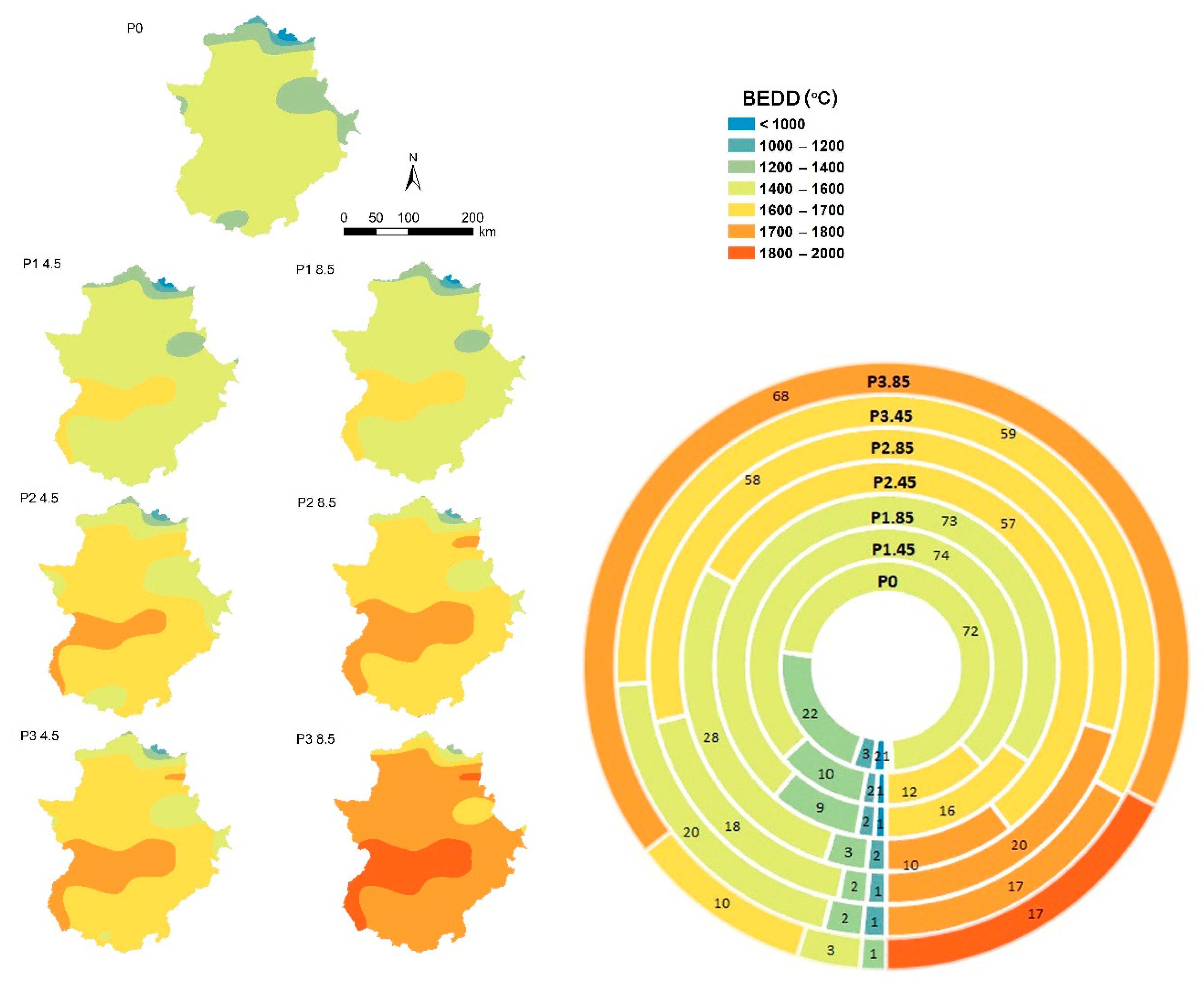
2.3. Bioclimatic Indices

GST, WI, HI and BEDD (Table 2) are commonly used because of their ability to describe cultivar suitability, the applicability for understanding wine region climate characteristics and the possibility of comparing between different regions. These four temperature-derived indices are a simple set of indicators of a climate suitable for the successful production of winegrapes in a region. It is important to emphasise that the conclusions in this study were drawn only by considering climatic variables. Non-climatic variables, for example, different geographical considerations such as the effect of topography on solar radiation interception, cultural practices to reduce the incidence of extreme climate conditions, or technology development, were not considered.
The GST is defined as the mean air temperature of all days between 1 April and 31 October (in the Northern Hemisphere), considering the active period of growth of the grapevine. Usually, GST should be between 13 and 21 °C for quality winegrape production [31]. This index provides the basis for placing latitudinal boundaries on viticulture areas [38].
The WI also denominated growing degree-days (GDD), is a daily effective thermal integral during the vegetative growing period. It is computed by subtracting a base temperature (commonly quantified as 10 °C for winegrapes) from the average daily temperature from 1 April to 31 October.
The HI considers an estimate of the daytime temperature by taking the maximum temperatures and the mean of the average in its calculations. Moreover, a length of day coefficient, K, is incorporated to consider the average daylight period for the latitude of the area. Huglin [32] developed this latitudinal correction for the latitudes of European viticulture as a linear response to increasing day lengths at higher latitudes. The HI is summed over a 6-month period, 1 April, and 30 September, rather than a 7-month period in the other indices since the heat accumulation in October are not considered important. K is 1.02 for 40° N latitude [5].
The BEDD index is another way to calculate heat summation, incorporating an adjustment for diurnal temperature range and a day length correction, as in the HI. However, in the BEDD index, the interval of effective heat summation is considered between 10 °C and 19 °C, base temperature, and upper threshold, respectively. Moreover, if the diurnal temperature range is greater than 13 °C, it is adjusted upward, and if less than 10 °C, downward. The coefficient K, length of the day, is similar to that applied to HI. The BEDD index is summed over 1 April and 31 October.

2.4. Statistical Analysis

Temporal trends in all bioclimatic indices were analysed by the Mann-Kendall test, as recommended by the World Meteorological Organisation [39]. Sen’s non-parametric method [40] determines the gradients and their direction. The relative change, RC, of each index throughout the studied period is identified following expression:
RC = (nβ/|x|) × 100
where n is the data set record length, β is the magnitude of trend in the time series and |x| is the absolute average value of the time series.
Comparisons between the three periods (P1, P2, and P3) and the past condition (P0) were performed for all bioclimatic indices under both RCP scenarios. The differences between each projected scenario and the reference period were computed. Statistically significant anomalies were assessed using the ANOVA test at a 5 % significance level for each grid point’s mean values. The null hypothesis indicates that data have the same mean, and the rejection of this null hypothesis addresses Tukey’s test. This multiple comparison procedure was used to find significantly different means between each period and the reference.
The spatial representation of all bioclimatic indices according to different scenarios was performed using the GIS software ArcGIS v.10.5 (ESRI Inc., Redlands, CA, USA). Figure 2 illustrates the overall methodological framework used in this study.

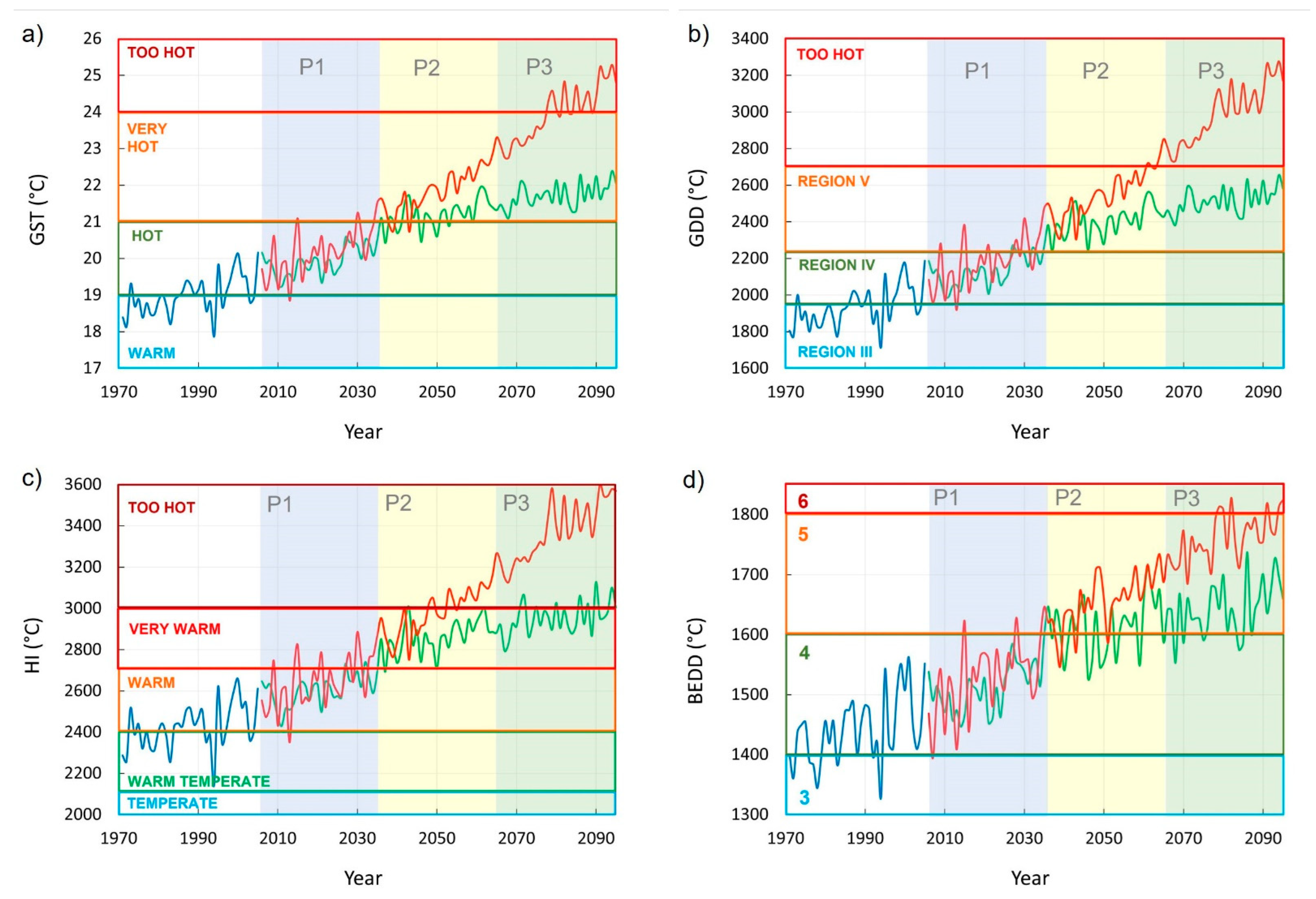
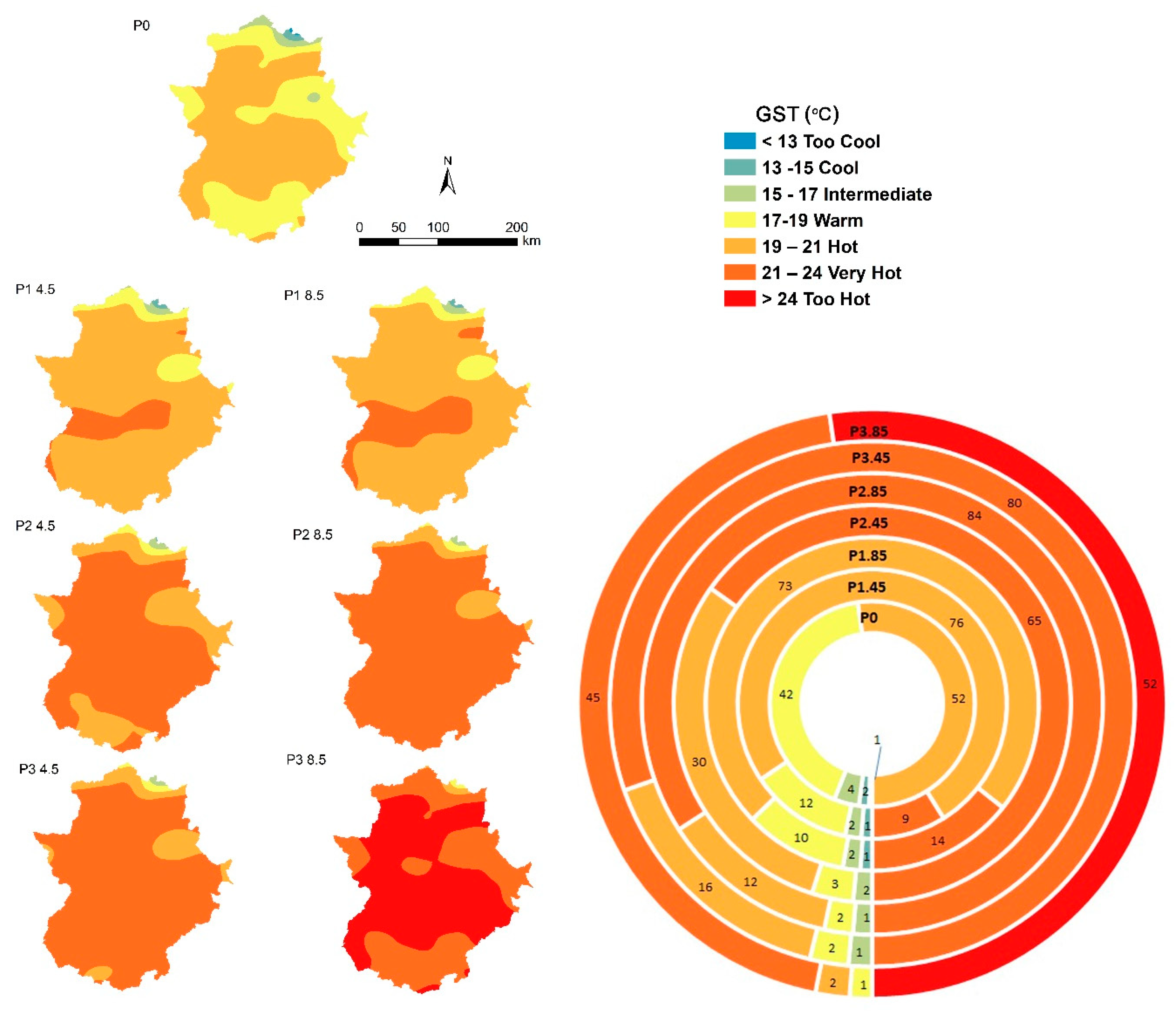
3. Results and Discussion

Temperature is one of the key climate variables for a vineyard; in consequence, warming could significantly impact winegrape production.
Table 3 outlines the mean indices for both the historical period, P0, and the three future periods, P1, P2, and P3, for both scenarios considered in the present study.
Throughout the 21st century, all mean indices should gradually increase, which will have a significant impact on future viticulture in the region. The graph in Figure 3 shows this increase over the years in future periods, particularly in the RCP 8.5 scenario, as expected. Both scenarios show a trend in period P1 similar to that observed in the historical period, with very similar values of annual increases. However, during period P2, the trends of the two scenarios begin to diverge. The RCP 8.5 scenario maintains an increasing trend similar to that of P1 in the following periods, P2 and P3, while the increasing trend is lower and even stabilises during the P3 period in the RCP 4.5 scenario.
As outlined in Table 4, both in the historical period and throughout the 21st century, all bioclimatic indices show significant change trends. In the RCP 4.5 scenario, the intensity of the change throughout the century will be very similar to that of the historical period because the Sen slopes are very similar. However, in the RCP 8.5 scenario, these intensities practically double, as do the Sen slopes. The relative change in the RCP 4.5 scenario is double that in the historical period, and the relative change in the RCP 8.5 scenario is double that in the RCP 4.5 scenario.
In Extremadura, the GST index, which is related to the optimal temperature ranges for vine development, was mainly found between the Warm and Hot classes in the P0 period (Figure 3a), as indicated by Honorio et al. [41] for the 1980–2010 period. As such, the region fell into optimal GST classes for viticulture. Extremadura produces wines of proven quality, mostly under the Ribera del Guadiana Protected Denomination of Origin, thus confirming the suitability of the region for wine production. As shown in Figure 3a, such conditions should be maintained in both scenarios until the end of period P1. However, for both scenarios in period P2, most of the region should be in the Very Hot category, which will only allow growing late-maturing varieties (Figure 3a and Figure 4). For the RCP 8.5 scenario, in period P3, the conditions will be Too Hot (Figure 3a and Figure 4), likely compromising high-quality grape production. Similar results were found by Teslić et al. [17] in the Emilia Romagna region (Italy) and by Koufos et al. [27] in Greece. As a result of this future increase in GST, phenological events will advance in Extremadura, as described by Fraga et al. [10], reaching up to 10 days in flowering and veraison and up to 20 days in ripening.
The Central West region (Las Vegas del Guadiana) will be the first area of Extremadura to experience Very Hot conditions for viticulture under both scenarios in period P1 (Figure 4). Subsequently, these conditions will extend to practically the entire autonomous community so that by the end of the century, the conditions will be Too Hot for viticulture in 52% of the territory under the RCP 8.5 scenario (Figure 4), including the current main wine-growing areas. However, in the RCP 4.5 scenario, despite the generalised warming, the conditions will not be Too Hot for viticulture. Nevertheless, Very Hot conditions will be reached across 80% of the territory (Figure 4), thereby requiring the adaptation of measures for quality viticulture [17].
The temporal evolution of the GDD (Figure 3b) in Extremadura shows a similar increasing GST trend, albeit with an approximately double RC (Table 4). Thus, starting from a Region IV category at the end of the historical period, the GDD should reach a Region V category in the RCP 4.5 scenario and Too Hot in the RCP 8.5 scenario by the end of the 21st century. Koufos et al. [42] found that the harvest date of all vine varieties under study will be bought forward because of the increase in GDD, particularly at the end of the 21st century, in the RCP 8.5 scenario. Similar results, albeit less intense, were found by Vukovic et al. [43] in Serbia and by Blanco-Ward et al. [44] in the Douro region of Portugal.
As shown by the spatial distribution of GDD in Figure 5, the Las Vegas del Guadiana area (Central West) will likely have the highest GDD values in the P1 period and for both scenarios. Therefore, warming mitigation measures must be implemented in this important viticultural area. For the RCP 4.5 scenario, in period P3, only Las Vegas del Guadiana should reach conditions classified as Too Hot, accounting for 13% of the total area (Figure 5). However, based on the projection for the RCP 8.5 scenario, by the end of the 21st century, virtually the entire region will be classified as Too Hot for viticulture. In this case, the current wine-growing areas will fall into the Too Hot classification, requiring the adaptation of measures for these limiting conditions towards preserving the productivity of these wine-growing areas, as well as the typicity and quality of the wines [45].
The HI (Figure 3c) also shows an increasing trend in the historical period, reaching the Warm category by the end of this period. In the following periods, and for both scenarios, its increase is evident, particularly in the RCP 8.5 scenario in which the class Too Hot will be reached in the mid-21st century. However, in the RCP 4.5 scenario, although the category Very Warm will be reached at the beginning of the P2 period, the class Too Hot will only be reached at the end of P3, that is, at the end of the 21st century. Thus, under Too Hot conditions, viticulture could be questionable.
Similar results were found by Teslić et al. [17] in the Emilia-Romagna region (Italy). However, in the RCP 4.5 scenario, the conditions will allow viticulture, albeit with adaptation measures [27], because the high temperatures will accelerate the phenological stages and shorten the growth intervals of vines, thereby affecting their quality [46].
Figure 6 shows the spatial distribution of HI, with 57% of the territory predominantly in the Warm condition during the historical period. However, in the RCP scenario 8.5, HI will gradually increase over time, reaching the category Very Warm in up to 34% of the territory in the P1 period and the category Too Hot in 51% of the territory in the P2 period, thus becoming the main class in this scenario. Towards the end of the 21st century, in the P3 period, the class Too Hot will extend almost throughout Extremadura, covering 95% of its land area in the RCP scenario 8.5 and a large area (39%) in the RCP 4.5 scenario.
As with the indices GST and GDD, HI should reach the highest values in the P1 period for both scenarios in the Las Vegas del Guadiana (Central West) zone. In this zone, in periods P2 and P3 and in scenario RCP 4.5, the category Too Hot will be reached. Therefore, as indicated before, the conditions will be unsuitable for viticulture.
The biologically effective degree-days (BEDD) index has the lowest RC values of the entire time series until the end of the 21st century for both scenarios (Table 4). For both scenarios, in the periods P0 and P1, BEDD values lie in the class 1400–1600 °C, reaching the class 1600–1700 °C in P2 and P3, as shown in Figure 3d. Similar results have been found in wine-growing areas of Greece by Koufos et al. [27], thus indicating that, if agronomic measures are not applied, primarily by selecting late-maturing varieties, grape ripening could be brought forward, falling outside the ideal period. This earlier ripening would cause an imbalance between the sugar concentration and acidity of musts. Conversely, this accelerated ripening could benefit high-altitude areas where grape ripening is currently compromised, as found by Eccel et al. [47] in the northern region of Italy.
As shown in Figure 7, the spatial distribution of the BEDD index in Extremadura during the historical period indicates that 1400–1600 °C is the predominant class, with other minor classes in a few areas to the north, south, and east of the region. In the P1 period, 1400–1600 °C will remain the predominant class, but with the 1600–1700 °C class in Las Vegas del Guadiana and with fewer zones with low values. For the RCP 4.5 scenario, in P2 and P3, the class 1600–1700 °C will prevail in the region, but in Las Vegas del Guadiana, the predominant class will be 1700–1800 °C. For the RCP 8.5 scenario, in the same periods, the zone with the 1600–1700 °C class will gradually extend across Extremadura and Las Vegas del Guadiana, reaching the 1800–2000 °C class by the end of the 21st century. In other words, the classes 1700–1800 °C and 1800–2000 °C will cover most of the Extremadura territory (approximately 85%) by them (Figure 7). Consequently, for this scenario, only the high-altitude areas would be appropriate to continue using the current varieties and cultivation techniques. However, for the low emissions scenario, only Las Vegas del Guadiana would reach very high ripening classes, with the ideal area for correct ripening accounting for 79% of the total territory of the region (Figure 7).
The statistical analysis of the differences between the scenarios for each future period and the baseline climate for all bioclimatic indices indicated significant changes in all cases. Consequently, the changes in the spatial variability of the bioclimatic indices indicate a clear increase in all their values until the end of the 21st century, particularly for the RCP 8.5 scenario. These changes will have a critical impact on viticulture in Extremadura, especially in the current wine-growing areas with the largest vineyard areas. In a study conducted in European wine-growing areas, Moriondo et al. [48] determined that heat accumulation indices, such as GDD, HI, and BEDD, reached their highest values in Extremadura (1950–2000 period), specifically in the PDO areas of Ribera del Guadiana. This study predicted that the vineyard area of Extremadura would decrease considerably because of the loss of climatic suitability for viticulture in the region. The present study, conducted with a higher spatial resolution, confirmed the harmful effects that a rise in temperature resulting from climate change would have on viticulture in Extremadura, highlighting changes in the climatic zoning of the region as the climate changes during this century, varying and decreasing the optimal areas for viticulture.
It is well known how higher temperatures affect winegrapes and the wine industry. For instance, earlier occurrence of phenological events [49], lower grape acidity at harvest [50], and an alcohol increase in wines [51] are expected from warming. Moreover, higher temperatures affect a wide range of metabolites, and in particular flavonoids, which are key compounds for berry and wine quality. A decrease in total anthocyanins is reported by Gouot et al. [52]. Changes in flavours and antioxidant composition have also been reported by Pons et al. [53]. These shifts could alter the suitability of Extremadura for winegrape production, including the current areas where the main vineyards exist. Not only the quality of wines could be affected but also the number of winegrapes; harvest during the hotter summer days, with higher water stress, will cause a lower crop load [10]. In consequence, technological developments, such as the use of new winegrape varieties more resistant to drought stress and heat or the application of shading nets, will also be crucial to maintain viticulture in Extremadura in the future.
Currently, no preventive or adaptive measures are being conducted in Extremadura to adapt viticulture to climate change. The main adaptative strategies are (1) The selection of new areas for viticulture. If the use of current varieties continues, zones with higher elevation would have to be selected to maintain the number of winegrapes and the quality of wines. (2) Genetic improvement. If there is no possibility to select new high-altitude areas, it is necessary to obtain new varieties adapted to the expected climatic conditions, with a longer vegetative-productive cycle and grape ripening outside of the warmer periods. New varieties more resistant to droughts, with higher water use efficiency, would be necessary, as those that Coupel-Ledru et al. [54] found. The choice of more efficient and drought-tolerant rootstocks has been proposed as another adaptation measure [55]. (3) Crop management. The implementation of cultivation techniques aimed at increasing the soil water storage capacity, such as the increase of organic matter, no-till or minimum tillage techniques, and permanent or semi-permanent plant cover management, has shown a positive effect [56]. Vineyard rows can be oriented to the east to be less exposed during the warmest period of the day. Trellising modes will have to be adapted to decrease the temperature at the bunches of winegrapes, with a higher shading, as Tomasi et al. [57] reported using the Pergola training system. Moreover, canopy management is important, removing leaves earlier and using foliar antiperspirants to reduce transpiration by forming a clear and flexible film that reduces normal moisture loss due to leaf transpiration. This treatment is effective in reducing the sugar accumulation in the berry without a significant prejudice to the accumulation of phenolic compounds [58]. Another treatment is the kaolin (i.e., white clay mineral) application to reduce the negative effects of high temperatures and heat stress on canopy physiological processes, yield and fruit quality. The temperature on leaves is reduced by radiation reflection and lower transpiration. Results have shown that it is an effective technique, quick and simple to be applied, as well as economical since it is sufficient to spray only one side of each row (50 % of the vineyard) [59]. Finally, the use of controlled deficit irrigation can be implemented, applying less water at specific developmental stages such that there is little, if any, negative impact on the yield.

4. Conclusions

The bioclimatic indices analysed in this study show that changes in the Extremadura region in the coming decades will worsen the conditions for viticulture and grape quality, especially in the RCP 8.5 scenario. In this scenario, the ideal wine-growing area will markedly decrease, becoming restricted to high-altitude areas, to the north of the region. These changes in weather conditions will require adapting cultivation techniques, varieties, dates of field operations, and the use of different technological developments for quality and sustainable viticulture.
In general, of the two scenarios analysed in this study, RCP 4.5 shows a smaller increase in the indices from the P2 period, reaching high categories but not as extreme as those found in the RCP 8.5 scenario, according to which the conditions in Extremadura will be too warm for wine production by the end of the 21st century.
These changes will occur first in the zone of Las Vegas del Guadiana, located in the Central-West Extremadura region, which seems to forecast the predominant climatic category in Extremadura in future periods. Accordingly, climate change mitigation strategies should be tested in Las Vegas del Guadiana.
The intensity of changes in bioclimatic indices in the RCP 4.5 scenario is very similar to that of changes observed in the historical period (P0). This similarity could indicate that if the historical trend continues, the RCP 4.5 scenario is more likely to occur than the RCP 8.5 scenario. However, climate change is a non-linear system. Therefore, despite foreseeing a trend similar to that of the historical period, irreversible changes may be triggered, creating a feedback loop.
Although currently no preventive or adaptive measures are being conducted in Extremadura to adapt viticulture to climate change, it would be necessary to start implementing some primary strategies, such as the use of new areas for viticulture and new varieties adapted to the expected climatic conditions and the implementation of new cultivation techniques and treatments to reduce the impact of high temperatures.

Author Contributions

Conceptualization, F.J.M., C.A. and L.L.P.; methodology, F.J.M., and L.L.P.; formal analysis, A.G.-M. and C.A.; investigation, F.J.M., C.A., V.A., A.G.-M., L.L.P. and F.J.R.; resources, C.A., V.A., A.G.-M. and L.L.P.; data curation, C.A., V.A. and F.J.R.; writing—original draft preparation, F.J.M., C.A. and A.G.-M.; writing—review and editing, F.J.M.; visualization, C.A., V.A. and F.J.R.; supervision, F.J.M., A.G.-M. and L.L.P.; project administration, F.J.M.; funding acquisition, F.J.M. All authors have read and agreed to the published version of the manuscript.

Funding

This research was funded by the Junta de Extremadura and the European Regional Development Fund (ERDF) through the projects GR21006 (Research Group TIC008, “Alcántara”) and IB18001 (“Análisis y modelizacion del impacto del cambio climático sobre la distribución de zonas vitícolas en Extremadura”).

Institutional Review Board Statement

Not applicable.

Data Availability Statement

Not applicable.

Conflicts of Interest

The authors declare no conflict of interest.

References

  1. Ceglar, A.; Toreti, A.; Lecerf, R.; van der Velde, M.; Dentener, F. Impact of meteorological drivers on regional inter-annual crop yield variability in France. Agric. For. Meteorol. 2016, 216, 58–67. [Google Scholar] [CrossRef]
  2. Hannah, L.; Roehrdanz, P.R.; Ikegami, M.; Shepard, A.V.; Shaw, M.R.; Tabor, G.; Zhi, L.; Marquet, P.A.; Hijmans, R.J. Climate change, wine, and conservation. Proc. Natl. Acad. Sci. USA 2013, 110, 6907–6912. [Google Scholar] [CrossRef] [PubMed] [Green Version]
  3. Ashenfelter, O.; Storchmann, K. Climate Change and Wine: A Review of the Economic Implications. J. Wine Econ. 2016, 11, 105–138. [Google Scholar] [CrossRef]
  4. Drappier, J.; Thibon, C.; Rabot, A.; Geny-Denis, L. Relationship between wine composition and temperature: Impact on Bordeaux wine typicity in the context of global warming—Review. Crit. Rev. Food Sci. Nutr. 2019, 59, 14–30. [Google Scholar] [CrossRef]
  5. Jones, G.V.; Webb, L.B. Climate Change, Viticulture, and Wine: Challenges and Opportunities. J. Wine Res. 2010, 21, 103–106. [Google Scholar] [CrossRef]
  6. Kizildeniz, T.; Mekni, I.; Santesteban, H.; Pascual, I.; Morales, F.; Irigoyen, J.J. Effects of climate change including elevated CO2 concentration, temperature and water deficit on growth, water status, and yield quality of grapevine (Vitis vinifera L.) cultivars. Agric. Water Manag. 2015, 159, 155–164. [Google Scholar] [CrossRef] [Green Version]
  7. Martínez-Lüscher, J.; Kizildeniz, T.; Vucetic, V.; Dai, Z.; Luedeling, E.; van Leeuwen, C.; Gomès, E.; Pascual, I.; Irigoyen, J.J.; Morales, F.; et al. Sensitivity of grapevine phenology to water availability, temperature and CO2 concentration. Front. Environ. Sci. 2016, 4, 48. [Google Scholar] [CrossRef] [Green Version]
  8. Tomás, M.; Medrano, H.; Escalona, J.M.; Martorell, S.; Pou, A.; Ribas-Carbó, M.; Flexas, J. Variability of water use efficiency in grapevines. Environ. Exp. Bot. 2014, 103, 148–157. [Google Scholar] [CrossRef]
  9. Cardell, M.F.; Amengual, A.; Romero, R. Future effects of climate change on the suitability of wine grape production across Europe. Reg. Environ. Chang. 2019, 19, 2299–2310. [Google Scholar] [CrossRef]
  10. Fraga, H.; García de Cortázar Atauri, I.; Malheiro, A.C.; Santos, J.A. Modelling climate change impacts on viticultural yield, phenology and stress conditions in Europe. Glob. Chang. Biol. 2016, 22, 3774–3788. [Google Scholar] [CrossRef]
  11. Cook, B.I.; Wolkovich, E.M. Climate change decouples drought from early wine grape harvests in France. Nat. Clim. Chang. 2016, 6, 715–719. [Google Scholar] [CrossRef]
  12. Ruml, M.; Vuković, A.; Vujadinović, M.; Djurdjević, V.; Ranković-Vasić, Z.; Atanacković, Z.; Sivčev, B.; Marković, N.; Matijašević, S.; Petrović, N. On the use of regional climate models: Implications of climate change for viticulture in Serbia. Agric. For. Meteorol. 2012, 158–159, 53–62. [Google Scholar] [CrossRef]
  13. Galbreath, J. Climate Change Response: Evidence from the Margaret River Wine Region of Australia. Bus. Strategy Environ. 2014, 23, 89–104. [Google Scholar] [CrossRef]
  14. Jones, G.V.; Reid, R.; Vilks, A. Climate, Grapes, and Wine: Structure and Suitability in a Variable and Changing Climate. In The Geography of Wine; Dougherty, P., Ed.; Springer: Dordrecht, The Netherlands, 2012; pp. 109–133. [Google Scholar] [CrossRef]
  15. Lorenzo, M.N.; Taboada, J.J.; Lorenzo, J.F.; Ramos, A.M. Influence of climate on grape production and wine quality in the Rías Baixas, north-western Spain. Reg. Environ. Chang. 2013, 13, 887–896. [Google Scholar] [CrossRef]
  16. Costa, R.; Fraga, H.; Fonseca, A.; de Cortázar-Atauri, I.G.; Val, M.C.; Carlos, C.; Reis, S.; Santos, J.A. Grapevine phenology of cv. Touriga Franca and Touriga Nacional in the Douro wine region: Modelling and climate change projections. Agronomy 2019, 9, 210. [Google Scholar] [CrossRef] [Green Version]
  17. Teslić, N.; Vujadinović, M.; Ruml, M.; Ricci, A.; Vuković, A.; Parpinello, G.P.; Versari, A. Future climatic suitability of the Emilia-Romagna (Italy) region for grape production. Reg. Environ. Chang. 2019, 19, 599–614. [Google Scholar] [CrossRef]
  18. Comte, V.; Schneider, L.; Calanca, P.; Rebetez, M. Effects of climate change on bioclimatic indices in vineyards along Lake Neuchatel, Switzerland. Theor. Appl. Climatol. 2022, 147, 423–436. [Google Scholar] [CrossRef]
  19. International Organisation of Vine and Wine (OIV). Statistical Report on World Vitiviniculture. Available online: https://www.oiv.int/es/normas-y-documentos-tecnicos/analisis-estadisticos (accessed on 10 July 2022).
  20. Ministerio de Agricultura, Pesca y Alimentación. Estadísticas Agrarias: Agricultura. Available online: https://www.mapa.gob.es/es/estadistica/temas/estadisticas-agrarias/agricultura/default.aspx (accessed on 23 May 2022).
  21. Fraga, H.; García de Cortázar Atauri, I.; Malheiro, A.C.; Moutinho-Pereira, J.; Santos, J.A. Viticulture in Portugal: A review of recent trends and climate change projections. OENO One 2017, 51, 61–69. [Google Scholar] [CrossRef] [Green Version]
  22. Lazoglou, G.; Anagnostopoulou, C.; Koundouras, S. Climate change projections for Greek viticulture as simulated by a regional climate model. Theor. Appl. Climatol. 2018, 133, 551–567. [Google Scholar] [CrossRef]
  23. IPCC. Summary for Policymakers. In Global Warming of 1.5 °C. An IPCC Special Report on the Impacts of Global Warming of 1.5 °C Above Pre-Industrial Levels and Related Global Greenhouse Gas Emission Pathways, in the Context of Strengthening the Global Response to the Threat of Climate Change, Sustainable Development, and Efforts to Eradicate Poverty; Masson-Delmotte, V.P., Zhai, H.-O., Pörtner, D., Roberts, J., Skea, P.R., Shukla, A., Pirani, W., Moufouma-Okia, C., Péan, R., Pidcock, S., et al., Eds.; World Meteorological Organization: Geneva, Switzerland, 2018; p. 32. [Google Scholar]
  24. Stocker, T.F.; Qin, D.; Plattner, G.; Alexander, L.; Allen, S.; Bindoff, N.; Bréon, F.; Church, J.; Cubasch, U.; Emori, S.; et al. Technical Summary. In Climate Change 2013: The Physical Science Basis; Contribution of Working Group I; Cambridge University Press: Cambridge, UK, 2014. [Google Scholar]
  25. Amblar, P.; Casado, M.J.; Pastor, A.; Ramos, P.; Rodríguez, E. Guía de Escenarios Regionalizados de Cambio Climático Sobre España a Partir de los Resultados del IPCC-AR5; Ministerio de Agricultura y Pesca, Alimentación y Medio Ambiente, Agencia Estatal de Meteorología: Madrid, Spain, 2017. [Google Scholar] [CrossRef]
  26. Jacob, D.; Petersen, J.; Eggert, B.; Alias, A.; Christensen, O.B.; Bouwer, L.M.; Braun, A.; Colette, A.; Déqué, M.; Georgievski, G.; et al. EURO-CORDEX: New high-resolution climate change projections for European impact research. Reg. Environ. Chang. 2014, 14, 563–578. [Google Scholar] [CrossRef]
  27. Koufos, G.C.; Mavromatis, T.; Koundouras, S.; Jones, G.V. Response o fviticulture-related climatic indices and zoning to historical and future climate conditions in Greece. Int. J. Climatol. 2017, 38, 2097–2111. [Google Scholar] [CrossRef]
  28. Santos, J.A.; Costa, R.; Fraga, H. New insights into thermal growing conditions of Portuguese grapevine varieties under changing climates. Theor. Appl. Climatol. 2019, 135, 1215–1226. [Google Scholar] [CrossRef]
  29. Moral, F.J.; Rebollo, F.J.; Paniagua, L.L.; García, A. Climatic spatial variability in Extremadura (Spain) based on viticultural bioclimatic indices. Int. J. Biometeorol. 2014, 58, 2139–2152. [Google Scholar] [CrossRef] [PubMed]
  30. Winkler, A.J.; Cook, J.; Kliewer, W.M.; Lider, L.A. General Viticulture. University of California Press: Berkeley, CA, USA, 1974. [Google Scholar]
  31. Jones, G.V. Climate and Terroir: Impacts of Climate Variability and Change on Wine, in Fine Wine and Terroir. In The Geoscience Perspective; Geoscience Canada Reprint Series, Number 9; Macqueen, R.W., Meinert, L.D., Eds.; Geological Association of Canada: St. John’s, NL, Canada, 2006; pp. 203–216. [Google Scholar]
  32. Huglin, P. Nouveau mode d’évaluation des possibilités héliothermiques d’un milieu viticole. Comptes Rendus De L’académie D’agriculture De Fr. 1978, 64, 1117–1126. [Google Scholar]
  33. Gladstones, J. Climate and Australian viticulture. Vitic. Resour. 1992, 1, 90–118. [Google Scholar]
  34. Anderson, J.D.; Jones, G.V.; Tait, A.; Hall, A.; Trought, M.T.C. Analysis of viticulture region climate structure and suitability in New Zealand. Int. J. Vine Wine Sci. 2012, 49, 149–165. [Google Scholar] [CrossRef] [Green Version]
  35. Moral, F.J.; Rebollo, F.J.; Paniagua, L.L.; García, A.; Honorio, F. Integration of climatic indices in an objetive probabilistic model for establishing and mapping viticultural climatic zones in a region. Theor. Appl. Climatol. 2016, 124, 1033–1043. [Google Scholar] [CrossRef]
  36. Aemet, I.M. Iberian Climate Atlas. Air Temperature and Precipitation (1971–2000); Ministerio de Medio Ambiente, y Medio Rural y Marino. Agencia Estatal de Meteorología e Instituto de Meteorología de Portugal: Madrid, Spain, 2011. [Google Scholar] [CrossRef]
  37. Observatorio Español del Mercado del Vino. Available online: https://www.oemv.es/superficie-de-vinedo-en-espana-ano-2020 (accessed on 15 June 2022).
  38. Gladstones, J. Climate and Australian Viticulture. In Viticulture, Volume 1. Resources, 2nd ed.; Coombe, B., Dry, P., Eds.; Winetitles: Adelaide, Australia, 2004; pp. 90–118. [Google Scholar]
  39. WMO (World Meteorological Organization). Guide to Hydrological Practices. Volume II—Management of Water Resources and Application of Hydrological Practices, 6th ed.; WMO-No. 168; World Meteorological Organization: Geneva, Switzerland, 2009. [Google Scholar]
  40. Sen, P.K. Estimates of the Regression Coefficient Based on Kendall’s Tau. J. Am. Stat. Assoc. 1968, 63, 1379–1389. [Google Scholar] [CrossRef]
  41. Honorio, F.; García-Martín, A.; Moral, F.J.; Paniagua, L.L.; Rebollo, F.J. Spanish vineyard classification according to bioclimatic indexes. Aust. J. Grape Wine Res. 2018, 24, 335–344. [Google Scholar] [CrossRef]
  42. Koufos, G.C.; Mavromatis, T.; Koundouras, S.; Jones, G.V. Adaptive capacity of winegrape varieties cultivated in Greece to climate change: Current trends and future projections. OENO One 2020, 54, 1201–1219. [Google Scholar] [CrossRef]
  43. Vukovic, A.; Vujadinovic, M.; Ruml, M.; Rankovic-Vasic, Z.; Przic, Z.; Beslic, Z.; Matijasevic, S.; Vujovic, D.; Todic, S.; Markovic, N.; et al. Implementation of climate change science in viticulture sustainable development planning in Serbia. E3S Web Conf. 2018, 50. [Google Scholar] [CrossRef]
  44. Blanco-Ward, D.; Ribeiro, A.; Barreales, D.; Castro, J.; Verdial, J.; Feliciano, M.; Viceto, C.; Rocha, A.; Carlos, C.; Silveira, C.; et al. Climate change potential effects on grapevine bioclimatic indices: A case study for the Portuguese demarcated Douro Region (Portugal). BIO Web Conf. 2019, 12, 01013. [Google Scholar] [CrossRef] [Green Version]
  45. Neethling, E.; Petitjean, T.; Quénol, H.; Barbeau, G. Assessing local climate vulnerability and winegrowers’ adaptive processes in the context of climate change. Mitig. Adapt. Strateg. Glob. Chang. 2017, 22, 777–803. [Google Scholar] [CrossRef]
  46. Lereboullet, A.-L.; Beltrando, G.; Bardsley, D.K.; Rouvellac, E. The viticultural system and climate change: Coping with long-term trends in temperature and rainfall in Roussillon, France. Reg. Environ. Chang. 2014, 14, 1951–1966. [Google Scholar] [CrossRef]
  47. Eccel, E.; Zollo, A.L.; Mercogliano, P.; Zorer, R. Simulations of quantitative shift in bio-climatic indices in the viticultural areas of Trentino (Italian Alps) by an open source R package. Comput. Electron. Agric. 2016, 127, 92–100. [Google Scholar] [CrossRef]
  48. Moriondo, M.; Jones, G.V.; Bois, B.; Dibari, C.; Ferrise, R.; Trombi, G.; Bindi, M. Projected shifts of wine regions in response to climate change. Clim. Chang. 2013, 119, 825–839. [Google Scholar] [CrossRef]
  49. Ruml, M.; Korać, N.; Vujadinović, M.; Vuković, A.; Ivanišević, D. Response of grapevine phenology to recent temperature change and variability in the wine-producing area of Sremski Karlovci, Serbia. J. Agric. Sci. 2016, 154, 186–206. [Google Scholar] [CrossRef]
  50. Bock, A.; Sparks, T.; Estrella, N.; Menzel, A. Changes in the phenology and composition of wine from Franconia, Germany. Clim. Res. 2011, 50, 69–81. [Google Scholar] [CrossRef] [Green Version]
  51. Teslić, N.; Zinzani, G.; Parpinello, G.P.; Versari, A. Climate change trends, grape production, and potential alcohol concentration in wine from the BRomagna Sangiovese appellation area (Italy). Theor. Appl. Climatol. 2018, 131, 793–803. [Google Scholar] [CrossRef]
  52. Gouot, J.C.; Smith, J.P.; Holzapfel, B.P.; Walker, A.R.; Barril, C. Grape berry flavonoids: A review of their biochemical responses to high and extreme high temperatures. J. Exp. Bot. 2019, 70, 397–423. [Google Scholar] [CrossRef]
  53. Pons, A.; Allamy, L.; Schüttler, A.; Rauhut, D.; Thibon, C.; Darriet, P. What is the expected impact of climate change on wine aroma compounds and their precursors in grape? OENO One 2017, 51, 141–146. [Google Scholar] [CrossRef] [Green Version]
  54. Couple-Ledru, A.; Lebon, E.; Christophe, A.; Doligez, A.; Cabrera-Bosquet, L.L.; Péchier, P.; Hamard, P.; This, P.; Simonneau, T. Genetic variation in a grapevine progeny (Vitis vinifera L. cvs Grenache × Syrah) reveals inconsistencies between maintenance of daytime leaf water potential and response of transpiration rate under drought. J. Exp. Bot. 2014, 65, 6205–6218. [Google Scholar] [CrossRef] [PubMed] [Green Version]
  55. Berdeja, M.; Nicolas, P.; Kappel, C.; Dai, Z.W.; Hilbert, G.; Peccoux, A.; Lafontaine, M.; Ollat, N.; Gomès, E.; Delrot, S. Water limitation and rootstock genotype interact to alter grape berry metabolism through transcriptome reprogramming. Hortic. Res. 2015, 2, 15012. [Google Scholar] [CrossRef] [PubMed]
  56. Judit, G.; Gabor, Z.; Adam, D.; Tamas, V.; Gyorgy, B. Comparison of three soil management methods in the Tokaj wine regio. Mitt Klosterneubg. 2011, 61, 187–195. [Google Scholar]
  57. Tomasi, D.; Calò, A.; Pascarella, G.; Pitacco, A.; Borsa, D.; Gaiotti, F. Effetti Dell’incremento Termico Sulla Qualità Aromatica Dell’uva: Il Caso Della Garganega e Delle Sue Forme di Allevamento; Quaderni CRA Istituto Sperimentale per la Viticoltura: San Michele all’Adige, Italy, 2015. [Google Scholar]
  58. Palliotti, A.; Poni, S.; Petoumenou, D.; Vignaroli, S. Limitazione modulata della capacità fotoassimilativa delle fogliemediante l’uso di antitraspiranti ed effetti su quantità e composizione dell’uva. II Convegno nazionale di Viticoltura, Marsala (TP). Italus Hortus 2010, 17 (Suppl. 3), 21–26. [Google Scholar]
  59. Palliotti, A.; Frioni, T.; Leoni, F. Caolino a effetto sunscreen. Vigne Vini Qual. 2017, 1, 42–48. [Google Scholar]
Figure 1. Location map of Extremadura. Digital elevation models and vineyards in Extremadura are shown (a). Grid points where climate variables were available and considered to calculate bioclimatic indices are indicated as crosses (b).
Agriculture 12 01865 g001
Figure 2. The overall methodological framework of this study.
Agriculture 12 01865 g002
Figure 3. Temporal evolution of GST (a), GDD (b), HI (c) and BEDD (d) during the historical period (blue line) and the future time periods considered in the study, under the RCP 4.5 (green line) and RCP 8.5 (red line) scenarios.
Agriculture 12 01865 g003
Figure 4. Spatial distributions of GST during the historical period (P0) and the future time periods (P1, P2 and P3) in Extremadura. The percentages of each GST class for all time periods and under both scenarios, RCP 4.5 and RCP 8.5, are also shown (for instance, P1.45 means the time period P1 under the scenario RCP 4.5).
Agriculture 12 01865 g004
Figure 5. Spatial distributions of GDD during the historical period (P0) and the future time periods (P1, P2 and P3) in Extremadura. The percentages of each GDD class for all time periods and under both scenarios, RCP 4.5 and RCP 8.5, are also shown (for instance, P1.45 means the time period P1 under the scenario RCP 4.5).
Agriculture 12 01865 g005
Figure 6. Spatial distributions of HI during the historical period (P0) and the future time periods (P1, P2 and P3) in Extremadura. The percentages of each HI class for all time periods and under both scenarios, RCP 4.5 and RCP 8.5, are also shown (for instance, P1.45 means the time period P1 under the scenario RCP 4.5).
Agriculture 12 01865 g006
Figure 7. Spatial distributions of BEDD during the historical period (P0) and the future time periods (P1, P2 and P3) in Extremadura. The percentages of each BEDD class for all time periods and under both scenarios, RCP 4.5 and RCP 8.5, are also shown (for instance, P1.45 means the time period P1 under the scenario RCP 4.5).
Agriculture 12 01865 g007
Table 1. Combinations of the Global Climate Models (GCM) and the Regional Climate Models (RCM) were used in this study.
Global ModelRegional Model
CCLM4-8-17RCA4RACMO22EREMO2009
CNRM-CM5XX
EC-EARTH X
IPSL-CM5A-MR X
MPI-ESM-LRXX X
MOHC-HadGEM2-ESXXX
Table 2. Temperature-derived indices used in the study.
IndexEquationMonthsClass Limits
GST d = 1 n T m a x + T m i n 2 n   1 April–
31 October
(1)
Too Cool < 13 °C
(2)
Cool = 13–15 °C
(3)
Intermediate = 15–17 °C
(4)
Warm = 17–19 °C
(5)
Hot = 19–21 °C
(6)
Very Hot = 21–24 °C
(7)
Too Hot > 24 °C
GDD
or
WI
d = 1 n m a x T m a x + T m i n 2 10 , 0 1 April–
31 October
(1)
Too Cool < 850
(2)
(Region I) 850–1389
(3)
(Region II) 1389–1667
(4)
(Region III) 1667–1944
(5)
(Region IV) 1944–2222
(6)
(Region V) 2222–2700
(7)
Too Hot > 2700
HI d = 1 n m a x T m e a n 10 + T m a x 10 2 , 0 K
where K is an adjustment for latitude/day
length
1 April–
30 September
(1)
Too Cool < 1200
(2)
Very Cool = 1200–1500
(3)
Cool = 1500–1800
(4)
Temperate = 1800–2100
(5)
Warm Temperate = 2100–2400
(6)
Warm = 2400–2700
(7)
Very Warm = 2700–3000
(8)
Too Hot > 3000
BEDD d = 1 n m i n M a x T m a x + T m i n 2 10 , 0 K + D R T a d j , 9
where
D T R a d j = 0.25 T m a x + T m i n 13 ,   T m a x T m i n > 13 0 ,     10 < T m a x T m i n < 13 0.25 T m a x + T m i n 10 ,   T m a x T m i n > 10
and K is an adjustment for latitude/day length
1 April–
31 October
(1)
<1000
(2)
1000–1200
(3)
1200–1400
(4)
1400–1600
(5)
1600–1700
(6)
1700–1800
(7)
1800–2000
(8)
>2000
Table 3. Mean and coefficient of variation for each bioclimatic index (°C units) and for each period and scenario.
GSTGDDHIBEDD
Historical PeriodP0 (1971–2005)Mean19.01935.82426.41442.8
CV (%)9.118.314.612.6
RCP 4.5P1 (2006–2035)Mean19.92132.12604.51511.6
CV (%)9.017.414.011.6
P2 (2036–2065)Mean21.22404.62863.51612.7
CV (%)9.116.913.710.1
P3(2066–2095)Mean21.72516.62954.91643.3
CV (%)9.216.914.010.1
RCP 8.5P1 (2006–2035)Mean20.22184.92644.81528.4
CV (%)9.418.114.311.4
P2 (2036–2065)Mean21.92555.22989.71656.4
CV (%)9.317.013.79.3
P3(2066–2095)Mean24.02998.33377.81761.0
CV (%)9.315.913.27.4
Table 4. Statistics of the Mann-Kendall test (ZMK) and the magnitude of trends approximated by Sen’s estimator (β) for each bioclimatic index, considering the historical period and all years until the end of the 21st century for each scenario. RC is the relative change.
ZMKβRC (%)
Historical PeriodGST3.58 ***0.035.88
GDD3.66 ***6.8112.32
HI2.87 **5.517.95
BEDD2.84 **2.636.38
RCP 4.5GST10.18 ***0.0312.61
GDD10.22 ***6.2123.77
HI9.60 ***5.6518.12
BEDD8.15 ***2.1912.38
RCP 8.5GST12.19 ***0.0626.13
GDD12.19 ***13.6447.61
HI11.95 ***12.2036.56
BEDD11.14 ***3.7420.40
*** Significant trend at the 0.001 level; ** Significant trend at the 0.01 level.
Publisher’s Note: MDPI stays neutral with regard to jurisdictional claims in published maps and institutional affiliations.

