Experimentally Based Numerical Simulation of the Influence of the Agricultural Subsurface Drainage Pipe Geometric Structure on Drainage Flow

Abstract

The geometric structure of corrugated plastic pipes affects performance in agricultural subsurface drainage systems. To explore the influence of pipe geometry on flow field characteristics and the characterization of water movements, we developed a three-dimensional (3D) steady-state subsurface drainage model based on computational fluid dynamics (CFD). An analysis of the CFD and sand tank results indicated that the proposed model can accurately simulate the subsurface drainage process (R² = 0.99). The corrugation structure parameters of the drainpipe, including the outside diameter, corrugation valley width and corrugation height, were taken as the objects for this study, and the influence of corrugation parameters on drainage discharge was orthogonally analysed. During drainage, the soil water initially collects in the corrugation valley and then approximately ninety percent of the water flows into the pipe through the bottom perforations; increasing the contact face area between the corrugation valley and soil can increase the flow rate of the drainpipe and the water table height above the pipe, which decreases the intersection position of the pipe and water table. The results of the analysis of the range and variance of the orthogonal experiment showed that the order of the primary and secondary factors influencing the drainage discharge was the outside diameter, corrugation valley width and corrugation height, with the outside diameter being most critical influencing factor.

1. Introduction

Corrugated plastic pipes are usually made of polyvinyl chloride (PVC), high-polyethylene (HDPE) or polyethylene (PE), which have the characteristics of stable chemical properties, light weight, low temperature resistance and excellent mechanical properties, and the raw materials and corrugated profile wall of the pipes not only make them flexible, but also make the ring stiffness of the corrugated pipes better than that of straight-walled pipes with the same quantity of raw materials [1]. Corrugated plastic pipes were introduced to agricultural subsurface drainage in the early 1960s. With the rapid technological improvements and development of pipe materials and the installation of agricultural subsurface drainage systems, traditional subsurface drainage materials such as clay and concrete drainpipes have been gradually replaced by corrugated plastic pipes. This is because of the many advantages of corrugated plastic pipes, such as higher mechanical strength, easy storage and transport and easy installation. Corrugated plastic pipes have become the preferred standards for subsurface drainage pipes and have been widespread since the 1980s [2,3].

There are two types of corrugated plastic pipe mainly used in subsurface drainage systems on the market, i.e., single-wall corrugated pipe and double-wall corrugated pipe, and the corrugated profile includes sinusoidal corrugations, spiral corrugations and parallel corrugations. Currently, the most commonly used corrugated pipe in agricultural subsurface drainage is the parallel single-wall corrugated pipe, which has the special structure of a periodically distributed corrugated pipe wall. The valley of the corrugated pipe is located in the middle of the two corrugations, and there are perforations at the bottom of the valley in each corrugation. This structural distribution allows excess water remaining in soils to drain through the pipe [4]. As an important component of subsurface drainage, pipes are designed for collecting and transporting water in the soil; the pipe diameter, perforation shape and pattern and corrugation geometries are important geometric structural design parameters that influence the drainage performance and the mechanical properties of the drainpipe [5,6]. However, unreasonable geometric structural design for corrugated pipes can lead to the drainage efficiency of subsurface drainage systems failing to achieve design criteria for the control of waterlogging damage, farmland drainage or preventing saline–alkaline soil. It can even cause clogging pipes, which consequently decrease service life and increase maintenance costs [7]. Meanwhile, mechanical properties exceeding the design criteria are not conducive to large-scale popularization and promotion because of the increased costs during production, transportation and installation.

To define the exact relationship between agricultural subsurface drainage performance and pipe geometry structural parameters, many researchers have performed several studies in this field. Currently, field experiments, sand tank experiments, electrolytic analog studies and analytical studies are the major means of research. Li and Wu [8] conducted a field orthogonal experiment over two consecutive years to investigate the influence of three factors, namely, corrugated plastic pipe material, perforation pattern and envelope materials, on drainage performance and soil salinity drenching. The experimental results showed that a combination of a 3% perforation area and a single layer of nonwoven fabric envelope material had a better drainage effect. For steady-state flow, the water flow toward a subsurface drainage pipe is subject to vertical, horizontal, radial and entrance resistance, as proposed by Ernst [9]. However, entrance resistance, resistance of the disturbed soil and radial resistance are theoretical concepts and cannot be physically separated or separately measured in the field. Cavelaars [10] introduced the concepts of ‘approach flow resistance’ and ‘approach flow head loss’ for the flow in the approach region. According to Childs and Youngs [11], a real drain can be replaced by an ideal drain with a small radius, referred to as the ‘equivalent or effective drain radius’. The effective radius depends on the entrance resistance and can be used as an alternative to the entrance resistance. Dierickx [12] and Smedema and Rycroft [13] designed and conducted electrolytic analog and sand tank experiments individually, and the results all indicate that the ‘effective diameter’ of the clay pipe and concrete pipe is smaller than that of the corrugated plastic pipe. Stuyt and Dierickx [6] deemed that the ‘approach flow resistance’ was impacted by the geometry of the corrugation, and sinusoidal wave pattern corrugation was better than buck corrugation since it improved the flow condition. Oyarce and Gurovich [5] investigated the effects of the pipe perforation percentage, pipe diameter and envelop material on the drainage performance, ‘approach flow resistance’ and ‘effective diameter’ by sand tank experiments. The results showed that a combination of smaller pipe diameter, higher perforation percentage and envelope could increase the drainage performance. Bahceci and Nacar [14] proposed a new drain envelope concept that was developed to overcome the problems of clogging, sedimentation and root growth inside subsurface drainpipes, and then Alavi and Naseri [7] evaluated the drainage performance of this concept in saline–sodic soil in a soil tank model. Gaj and Madramootoo [15] used a numerical model to simulate the effects of perforation shape, size, and configuration on the entrance resistance and concluded that the use of rectangular slots is hydraulically more advantageous than circular holes in the valleys of corrugated pipes.

However, due to the limits of experimental conditions, field experiments and sand tank experiments are usually expensive, time consuming and labor intensive, and often, only a small number of samples can be gathered for qualitative studies of the geometry of pipes. Therefore, quantification research has not been satisfactorily carried out. Additionally, flow field characteristics cannot be easily measured and observed during field and sand tank experiments. In addition, many experimental factors have an impact on the research, including time, perforation, diameter, and filter material, presenting technical challenges for accurate measurements of the ‘effective diameter’ [16]. Although electrolytic analog studies have greatly increased the knowledge of subsurface drainage materials, the experimental setup and electrolytes used in the experiment do not match the complexity of real-world subsurface drainage situations [6].

Obtaining accurate and reasonable hydraulic characteristic data about a flow field is restricted by the experimental conditions and means of monitoring. Under the same experimental conditions, it is important to identify the influence of the geometric structure parameters of the pipe on drainage performance. However, the experimental conditions may be different between the two controlled trials, particularly under field conditions. Owing to the complexity of the manufacturing process of corrugated plastic pipes, it is difficult to fabricate different pipe structures and carry out subsurface drainage sand tank experiments.

To compensate for this deficiency, many scholars have begun to use numerical simulations to analyze subsurface drainage. There are many models for studying subsurface drainage; the most commonly used are HYDRUS [17], DRAINMOD [18] and SWAP [19,20]. The models have been widely used to simulate the dynamic processes of water and solute transport and to calculate the water table, drainage density and total volume of drainage with better performance [21,22,23]. These simulation models usually represent a pipe as an ‘ideal drain’ based on a continuously permeable wall that improves the description of the characterization of the flow field in drainage [24,25]. However, actual drainpipes are only permeable through the perforations on their walls, and water can only enter a real drain through a finite number of perforations. Additionally, DRAINMOD and SWAP are one-dimensional models but HYDRUS can simulate two-dimensional and three-dimensional water flow situation scenarios. However, the structural features of corrugation pipes cannot be fully considered when the seepage boundary is applied for subsurface pipes in HYDRUS-2D, which means that water immediately discharges when the surrounding soil is saturated [26]. The actual water flow in the approach region of the drainpipe cannot be described by only considering the seepage boundary.

Studying the influence of the pipe structural parameters on drainage performance requires an accurate structural description of the corrugated pipe and the water transport characteristics in the approach region of the drainpipe. CFD is a well-proven and economically feasible numerical method commonly used for predicting and simulating complex fluid flow and is widely used in fluid mechanical engineering, aerospace engineering and biological and medicinal applications [27]. CFD is a very important technology that can not only compensate for the limitations of field experiments, but also obtain numerous quantitative and qualitative data to solve complex flow problems. Lee and Bitog [28] reviewed the past, current and future directions of CFD in the agriculture sector, and the accuracy of the technique has been fully validated over a long history of development and applications. Afrin and Khan [29] developed an experimentally validated 3D model for the stage–discharge relationship of a perforated pipe aggregate system and analyzed the hydraulic performance under saturated and unsaturated flow conditions. Fu and Yang [30] established a mathematical model to detect and evaluate a single leakage in a fluid pipeline based on experimental study and 3D CFD simulation.

In the present study, to probe the hydraulic properties of the flow field during drainage, especially in the region close to the drainpipe, and to assess the pipe geometric structure’s impact on water movement characteristics, we constructed a 3D subsurface drainage model based on CFD. In this experiment, CFD models can compensate for the limitations and disadvantages of field experiments and obtain qualitative and quantitative flow field data. We validated the model by comparing it with sand tank subsurface drainage experimental data and revealed the hydraulic performance of closed pipes based on the CFD model. Then, through an orthogonal experiment (L₉(3⁴)), water seepage features near the pipe influenced by geometric structures were investigated. We used the experiment to evaluate the performance of drainpipes for drainage and to obtain the major influencing factors of the geometrical structure parameters that affect drainage efficiency. With this study, we have attempted to provide some usability recommendations for the optimization of corrugated plastic pipe geometric structure design for subsurface pipe drainage systems.

2. Materials and Methods

This study was carried out at The State Key Laboratory of Water Resources and Hydropower Engineering Science, Wuhan University. A subsurface drainage experiment was performed using a sand tank, and the experimental data were used to establish the geometric structure parameters of the CFD model, calibrate the parameters and verify the model. Since the process of field subsurface pipe drainage is usually unsteady, to better contrast the drainage performance of drainpipes, simplify the experiment and to analyze the results, in this study, subsurface pipe drainage was analyzed through steady-state drainage experiments. The constant water head method was adopted, and the water head height of the inlet was constant.

A steady-state 3D subsurface drainage model based on CFD was established in the present study, in which porous media were used to simulate soil resistance and the volume of fluid (VOF) method was used to simulate multiphase flows. Through the postprocessing visualization and analysis of the simulation results, the hydraulic characteristics of the subsurface drainage flow field were determined using CFD software. Figure 1 shows the procedure for the sand tank experiment and model simulation, including experimental arrangement, data collection, model calibration and validation and results analysis.

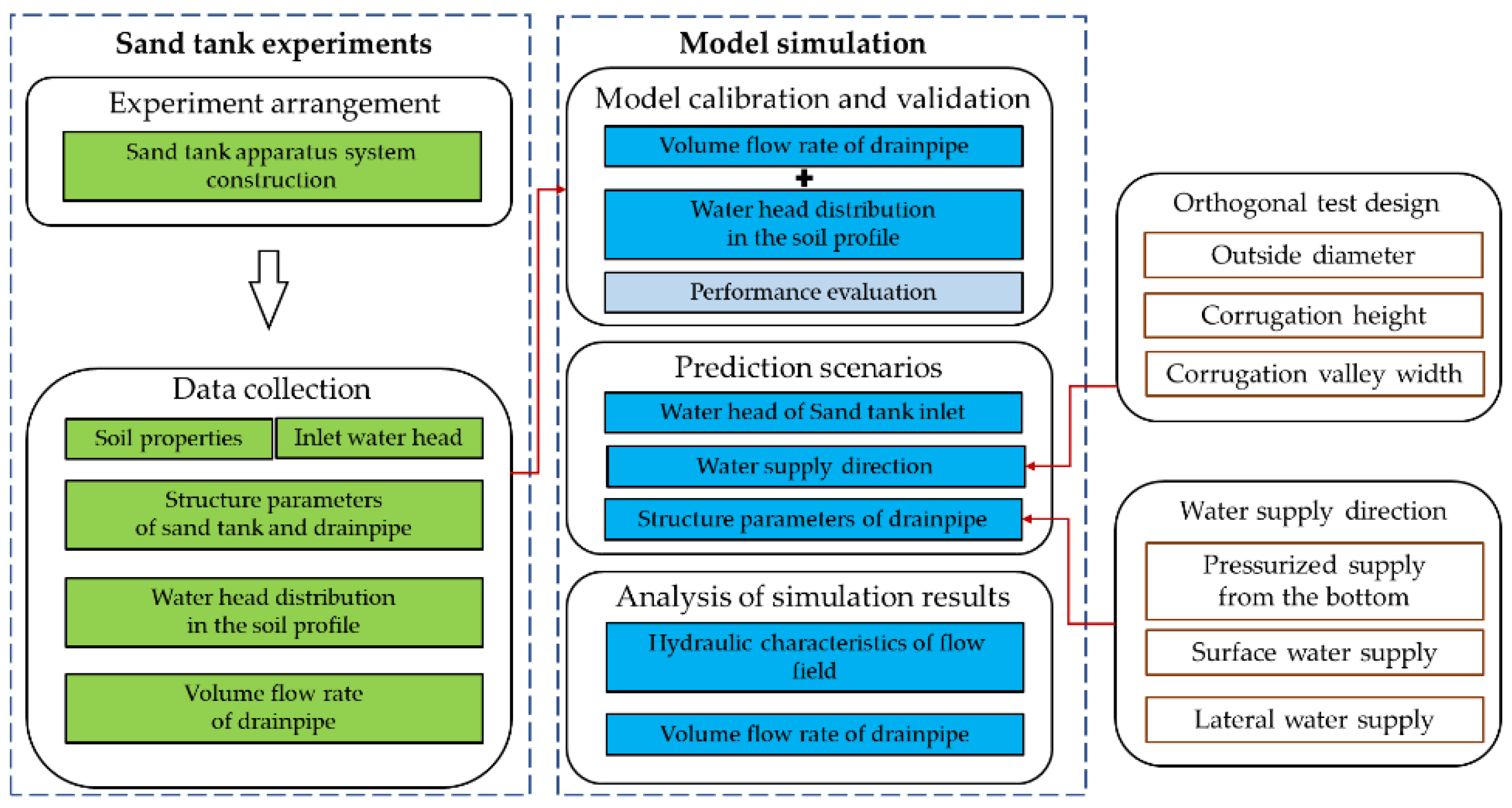
2.1. Sand Tank Drainage Experiment

2.1.1. Experimental Design

The experimental unit consisted mainly of a sand tank, an overflow tank, a plastic corrugated pipe and piezometer tubes. The sand tank, made of plexiglass and angle steel, had a cuboid shape (1.2 × 0.3 × 1.025 m³) and was connected to the overflow tank by three plastic catheters. The overflow tank was height-adjustable and provided a fixed water head pressure to the bottom of the sand tank. A 2.5 cm thick permeable plate was placed at the bottom of the sand tank, and a nonwoven fabric was laid on the upper part of the permeable plate to prevent the loss of soil in the sand tank. Piezometric tubes were arranged on the front of the sand tank to monitor the water head pressure at each position. The piezometric tubes near the drainage pipes were arranged in a double-cross shape, and the other piezometric tube distances in the transverse and longitudinal directions were 20 mm and 10 cm, respectively. A 9 cm diameter circular hole was opened in the middle of the plexiglass plate on the front of the sand tank. The distances between the center of the circular hole and the left, right and bottom of the sand trough were 60 cm, 60 cm and 42.5 cm, respectively. The corrugated pipe was installed here, and the buried depth was 50 cm. The arrangement of the sand tank and overflow tank and dimensions are shown in Figure 2.

The sand tank was filled with a medium coarse sand with soil particle sizes in the range of 0.25–1.00 mm and a mean bulk density of 1.6693 g/cm³. The soil particle size distribution is shown in Figure 3. Its soil saturated water content was 46.18%. The soil was loaded from the bottom of the sand tank until 9 layers were achieved, the thickness of each layer was 10 cm and the interface of each layer was rough.

The single-walled plastic pipes used in the research experiment were produced by Xinjiang Tianye (Group) Co. The perforation was placed in the valleys of the corrugation. The perforation was rectangular and three columns were arranged parallel with a spacing of 120-degree angles between columns. When fitting pipes, one column was positioned at the bottom of the pipe facing downward, and the other two were positioned at the shoulder section. The geometry and dimensions of the pipes are illustrated in Figure 4 and

Table 1. Corrugated pipe and perforation design used in the sand tank experiments.

Geometric Structural Parameters	Value
Outside diameter (mm)	90
Inside diameter (mm)	82
Wall thickness (mm)	1
Ridge width (mm)	5.35
Corrugation valley width (mm)	4
Corrugation height (mm)	4
Perforation length (mm)	26.67
Perforation width (mm)	0.6
Number of perforation rows	3
Perforation rate (%)	1.99
Total area of perforation per meter (cm2·m−1)	51

. One layer of geotextile covers the external surface of the corrugated pipes to prevent soil particles from entering the pipes. The outlet of the corrugated pipe was connected to a length of outflow tubing and the other end of the pipe was sealed tightly with rubber stoppers.

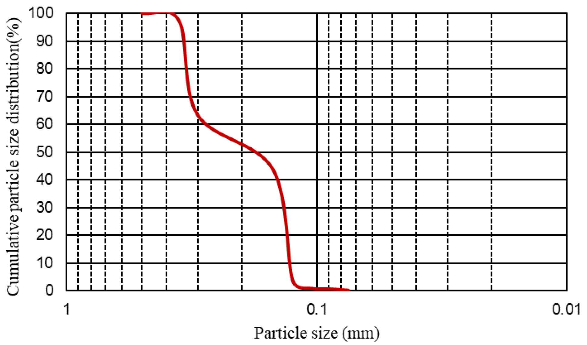
2.1.2. Experimental Measurement

After setting up the experimental device, the height of the overflow tank was adjusted and water was slowly supplied to the bottom of the sand tank until the water surface was flush with the surface of the soil on the top of the sand tank. The sand tank was left at rest for 24 h. Then, the air in the soil pores was vented. Then, the outlet of the pipes was slowly opened to allow the water to steadily flow. Subsequently, the height of the overflow tank was adjusted to the desired height. When the volume flow rate of the drainpipe stabilized, data collection was initiated. During these processes, the experimental water was supplied into the sand tank from the overflow tank driven by gravity and then drained from the soil via the drainpipe located in the middle of the sand tank.

2.2. Numerical Model

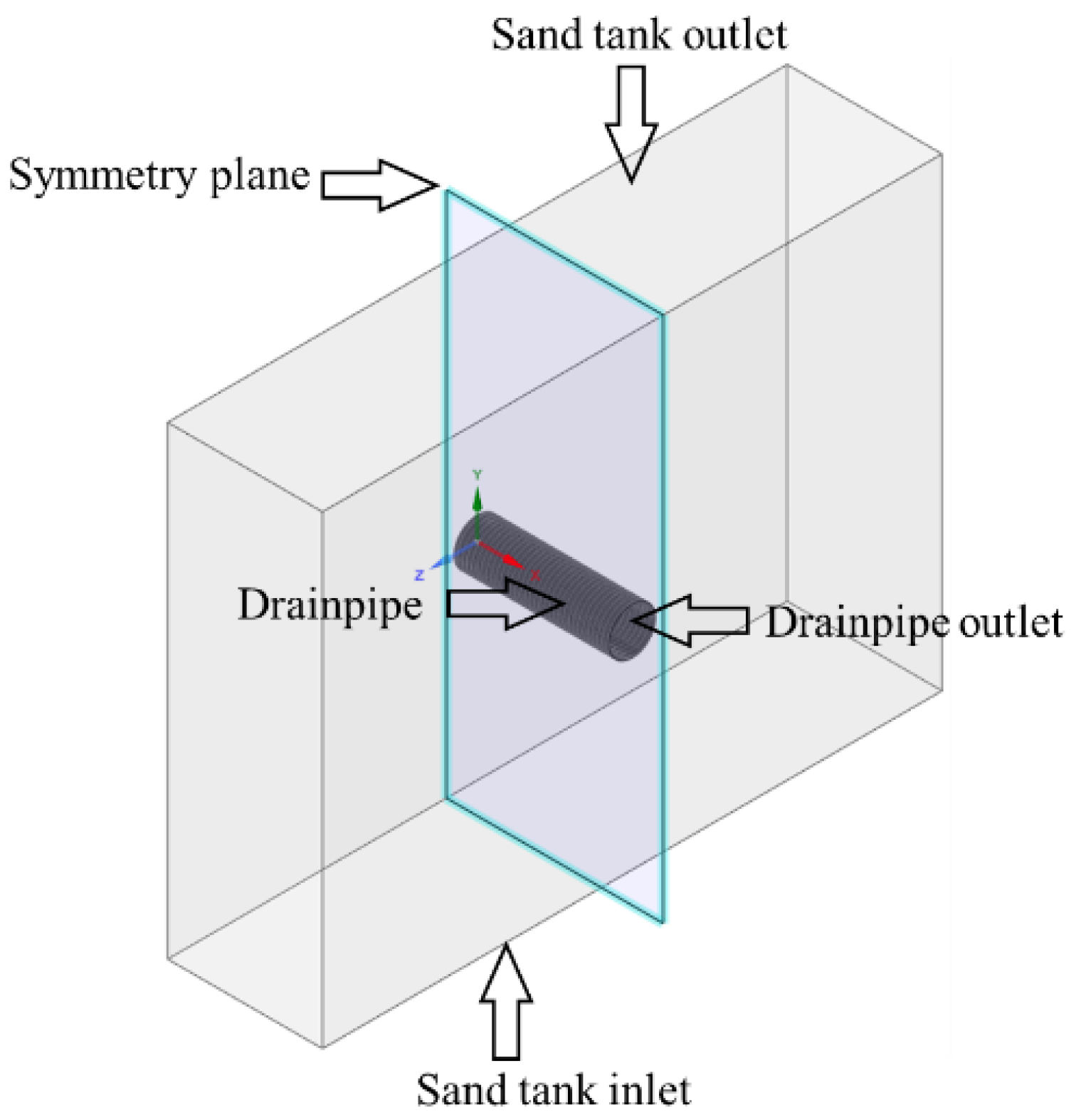
2.2.1. Numerical Modeling and Boundary Conditions

We performed subsurface drainage analysis with ANSYS Workbench and ANSYS Fluent software. To set up the CFD models, the computational domain was determined first. The finite volume method was applied to discretize the computational domain into computation cells. Then, the type of calculation model was selected, the fluid material was selected, various boundary conditions were set and the calculation was carried out.

2.2.2. Governing Equations

The flow simulation was based on solving the Navier–Stokes equations (momentum and mass conservation) for an incompressible fluid as follows [31].

Mass conservation equation:

$$\frac{\partial }{\partial t}\left(\rho \right)+\nabla \cdot \left(\rho \overrightarrow{v}\right)=0;$$

(1)

Momentum equation:

$$\frac{\partial }{\partial t}\left(\rho \overrightarrow{v}\right)+\nabla \cdot \left(\rho \overrightarrow{v}\overrightarrow{v}\right)=-\nabla p+\nabla \cdot \left[\mu \left(\nabla \overrightarrow{v}+\nabla {\overrightarrow{v}}^T\right)\right]+\rho \overrightarrow{g}+\overrightarrow{F}$$

(2)

where

$\rho =$ the density of fluid;

$u_i=$ components of the velocity vector;

$\mu =$ the fluid dynamic viscosity.

$$\rho ={\displaystyle \sum }_{i=1}^2{\alpha }_i{\rho }_i$$

(3)

$$\mu ={\displaystyle \sum }_{i=1}^2{\alpha }_i{\mu }_i$$

(4)

The VOF model, which is a Euler–Euler approach, was applied to address multiple phases: gas and water. The sum of volume fractions in all phases should equal one. The interface between the two phases in the VOF model was tracked by solving for the continuity of the volume fraction equation [32]:

$$\frac{\partial {\alpha }_w}{\partial t}+\overrightarrow{v}\cdot \nabla {\alpha }_w=0$$

(5)

where ${\alpha }_w$ is the volume fraction of water.

2.2.3. Computational Domain and Boundary Conditions

The modelled geometry consisted of three zones: the corrugated pipe, the soil and the air zone in the pipe. The size of the computational domain of the subsurface drainage model was kept the same as that of the sand tank. For the CFD models, a pressure inlet, two pressure outlets, a symmetry boundary and the rest of the boundaries were set to a no-slip wall, including the corrugated pipe wall. The boundary conditions are presented in Figure 5.

To conduct the CFD simulation, the permeability of the soil and envelop material in the sand tank experiment were initially estimated through a porous media model. The porous media model only adds a momentum sink to the governing momentum equations, generating pressure gradients in the porous media. The momentum sink term in the model for simple homogeneous porous media can be described as [33,34]:

$$F_i=\frac{v}{\alpha }{u}_i+\frac{1}{2}{C}_2\rho \left|u\right|u_j$$

(6)

where F is the momentum source and $\alpha$ and $C_2$ are the permeability and inertial resistance, respectively. In our study, the inertial resistance of the soil and envelope could be treated as zero because water flowed slowly within the entire soil and envelope.

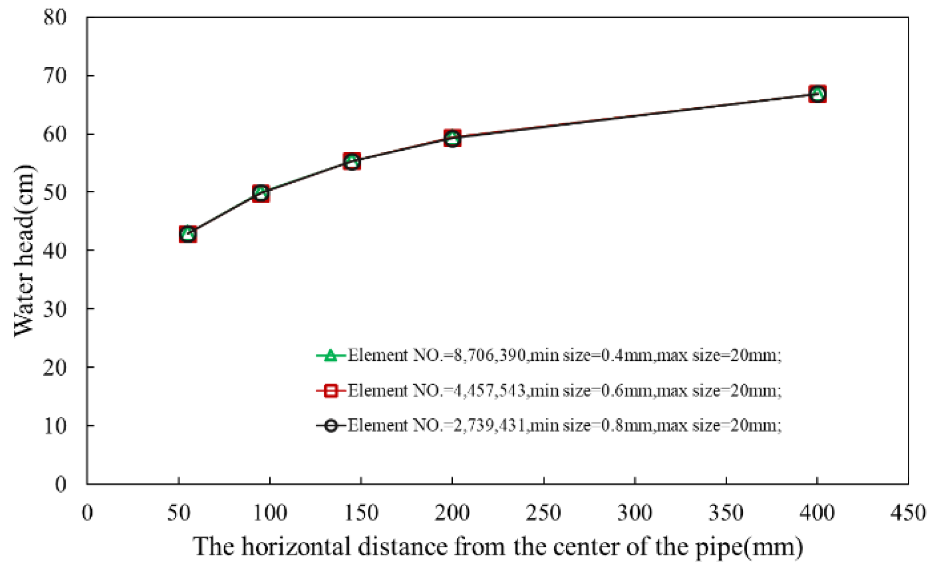
2.2.4. Grid Independent Test

The computational domains must be divided into cells, a process called discretization of the domain. Since grid density affects computational accuracy, the influence of the grid density on the CFD model was analysed. The mesh was chosen to be sufficiently fine to allow numerical convergence of the results. With an increasing number of mesh elements, the precision of the computational results is improved, while the complexity of the computation process also increases accordingly.

A mesh sensitivity analysis was performed to determine the minimum number of elements that could ensure grid-independent results. A polyhedral mesh and a prism layer mesh were selected for the analysis model, and with a maximum element size of 20 mm, the minimum element size increases gradually from 0.8 mm to 1.0 mm to 1.2 mm. More specifically, three different numbers of grids (1.3 million, 1.68 million and 2.4 million grid units) were used under the same simulation conditions for the calculation. An example of the mesh grids is shown in Figure 6.

The model was solved under the working condition that the constant water head of the inlet was 90 cm. Simulations were run until a steady state was reached. We set five monitoring points in which the horizontal distances from the center of the pipe were 55 mm, 95 mm, 125 mm, 200 mm and 400 mm and compared the results of the pressure head with three different numbers of grids. Figure 7 shows the result of the mesh sensitivity analysis conducted for the treatment with a 90 cm inlet water head pressure.

The grid independence evaluation revealed that there was little difference (<1%) in the calculation results with an increasing number of grids beyond a grid size of 8.70 million elements. The optimum number of cells was found to be 2,739,431, with a minimum element size of 0.8 mm and a maximum element size of 20 mm.

2.2.5. Model Validation and Evaluation

To validate the accuracy of the subsurface drainage CFD model, three working conditions of sand tank experiments were conducted. In addition to contrasting the simulation and experimental data, we evaluated the goodness-of-fit between simulated and experimental data and the performance of the models using common accuracy evaluation metrics, namely, the relative root mean square error (RRMSE), Nash–Sutcliffe efficiency coefficient (NSE) and the mean absolute error (MAE). The coefficient of determination (R²) is defined as follows:

$$\mathrm{M}\mathrm{A}\mathrm{E}=\frac{1}{n}{\displaystyle \sum }_{i=1}^n\left|f_i-y_i\right|$$

(7)

$$\mathrm{RRME}=\sqrt{\frac{{{\displaystyle \sum }}_{i=1}^n{\left(f_i-y_i\right)}^2}{n\times {\left(\frac{1}{n}{{\displaystyle \sum }}_{i=1}^n{f}_i\right)}^2}}$$

(8)

$$\mathrm{NSE}=1-\frac{{{\displaystyle \sum }}_{\overline{j}-1}^n{\left(f_i-y_{\mathrm{i}}\right)}^2}{{{\displaystyle \sum }}_{i=1}^n{\left(f_i-\overline{y}\right)}^2}$$

(9)

$${\mathrm{R}}^2=\frac{{\left({{\displaystyle \sum }}_{i=1}^n\left(y_i-\overline{y}\right)\left(f_i-\overline{f}\right)\right)}^2}{{{\displaystyle \sum }}_{i=1}^n{\left(y_i-\overline{y}\right)}^2{{\displaystyle \sum }}_{i-1}^n{\left(f_i-\overline{f}\right)}^2}$$

(10)

where $f_{i }$ is the simulated value, $y_i$ is the observed value, $\overline{y}$ is the averaged observed value and n is the sample size. An MAE value close to 0, an RRMSE value close to 0% and an NSE value close to 1.0 show model accuracy.

The outlet volume water flow rate measured by the sand tank experiment was compared with the CFD model simulation result to validate the effectiveness of the CFD model. The results show that the volume water flow rate of the outlet deviation between the experiment and the simulation was smaller than 6%, as shown in

Table 2. Comparison between the numerical and experimental outlet volume water flow rates.

Inlet Water Head (cm)	Outlet Volume Water Flow Rates (mL/s) (Experimental)	Outlet Volume Water Flow Rates (mL/s) (Numerical)	Deviation (%)
70	30.98	29.90	−3.49
80	40.35	41.02	1.66
90	50.33	53.32	5.94

. The MAE was 1.58 mL/s, the RRMSE was 4.5%,the NSE was 0.962, and the R² was 0.99. The deviations between the CFD model and the experiment may be caused by the random response of factors such as soil density inhomogeneities in the sand tank, soil capillary action, accuracy of device installation and other factors. Overall, the CFD model can satisfactorily describe the hydraulic performance of the sank tank subsurface drainage experiment.

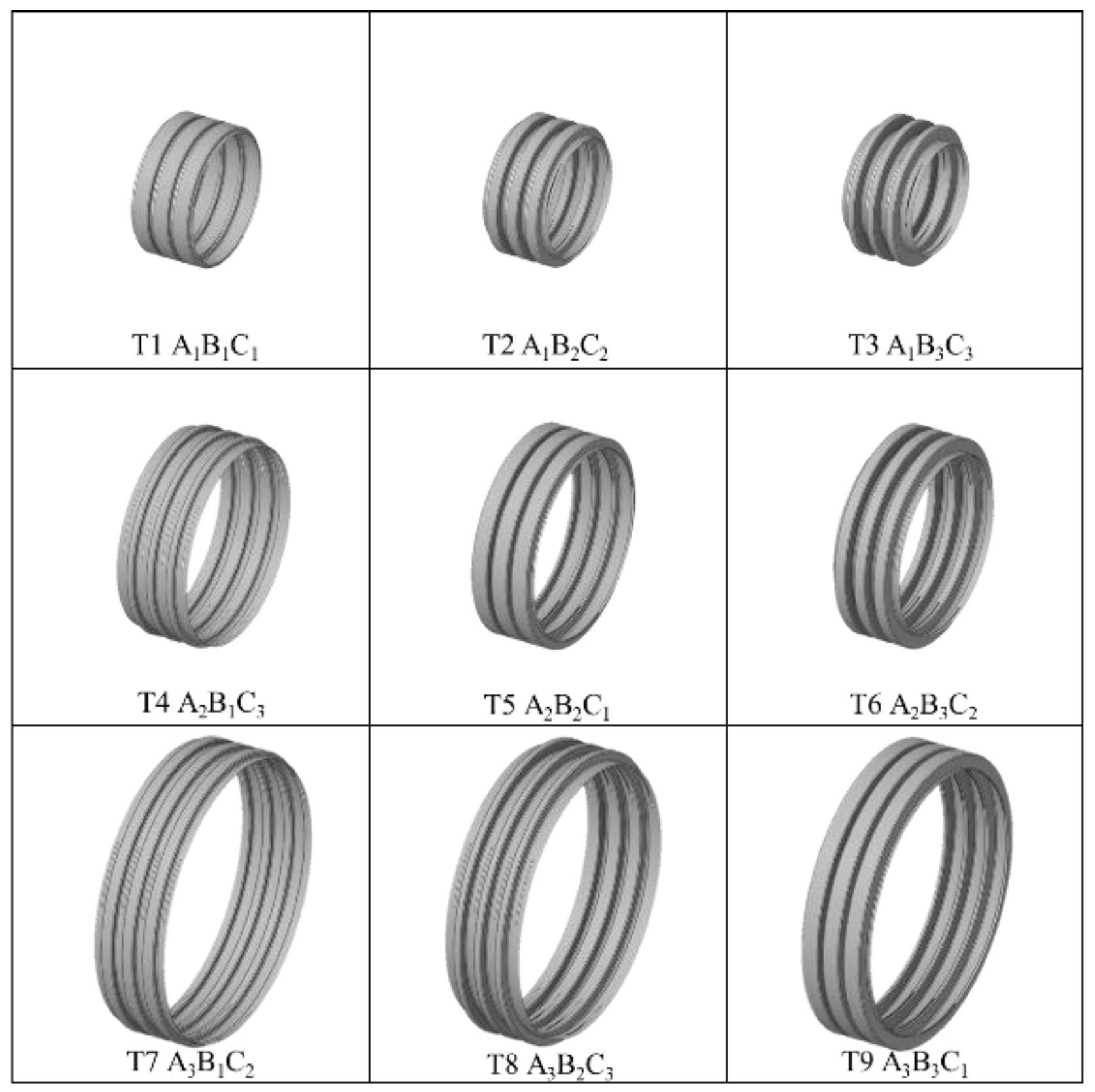
2.3. Orthogonal Test Design

The orthogonal experimental design method is a highly efficient, fast and economical experimental design method for evaluating the effects of various factors on drainage performance. To optimize the drainage performance of the corrugated pipe, several geometrical structural parameters were considered, including the outside diameter, corrugation height and corrugation valley width. An orthogonal L₉(3⁴) experiment with three factors and four levels was designed to determine the optimal pipe geometry structure parameters for drainage. The corrugation pitch for all treatments was 9.35 mm. The factors and levels are shown in

Table 3. Factors and levels.

Level	Factor A: Outside Diameter (mm)	Factor B: Corrugation Height (mm)	Factor C: Corrugation Valley Width (mm)	Blank
Level 1	60	2	2	1
Level 2	90	4	4	2
Level 3	120	6	6	3

. The orthogonal test design is shown in

Table 4. Orthogonal test design table (L₉(3⁴)).

Treatments	Factors				Experiment Scheme
	Factor A	Factor B	Factor C	Blank
T1	Level 1	Level 1	Level 1	Level 1	A1B1C1
T2	Level 1	Level 2	Level 2	Level 2	A1B2C2
T3	Level 1	Level 3	Level 3	Level 3	A1B3C3
T4	Level 2	Level 1	Level 3	Level 2	A2B1C3
T5	Level 2	Level 2	Level 1	Level 3	A2B2C1
T6	Level 2	Level 3	Level 2	Level 1	A2B3C2
T7	Level 3	Level 1	Level 2	Level 3	A3B1C2
T8	Level 3	Level 2	Level 3	Level 1	A3B2C3
T9	Level 3	Level 3	Level 1	Level 2	A3B3C1

and the corrugated pipe numerical models are shown in Figure 8.

3. Results

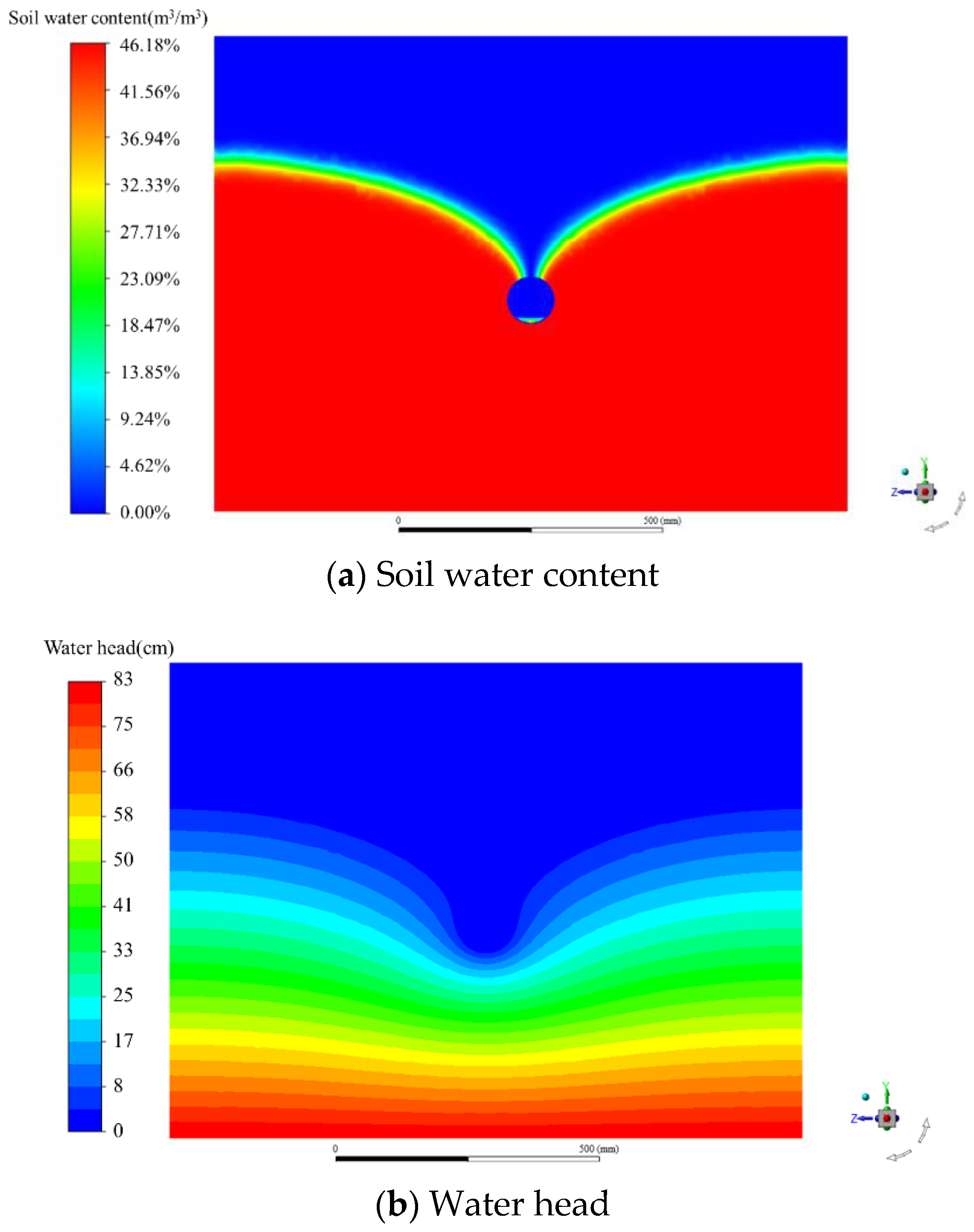
3.1. Hydraulic Properties of the Subsurface Drainage Flow Field

The inlet gauge pressure head at 90 cm, the outlet gauge pressure at zero and no-slip boundary conditions for all boundaries except inlet and outlet were set as initial conditions for the calculation. The results of CFD model analysis were visualized so that the hydraulic information in the flow field could be evaluated. The soil water content and water head distributions of the flow field were analysed. The results are presented via cloud charts. The soil water content distribution map and water head distribution map are shown in Figure 9a,b, respectively. Figure 9a shows the distribution of the saturated water table and the intersection position of the pipe and water table. Figure 9b shows the maximal water head at the bottom, which is the pressure inlet. The water head reduction near the pipe was significantly larger than that in the other flow fields.

We modeled three different pipe outside diameters and analyzed the soil water content, as illustrated separately in Figure 10. It can be seen from the figure that for three kinds of pipe outside diameters of 60 cm, 90 cm and 120 cm, the soil water content was substantially different, particularly the location of the water table heights and the intersection position of the pipe and water table. The larger the outside diameter is, the lower the water table and the intersection position. Due to the pressure in the subsurface drainage pipe and the insufficient section size of the drainpipe, a pressure head will be formed above the pipe, which we commonly refer to as the hanging curtain section.

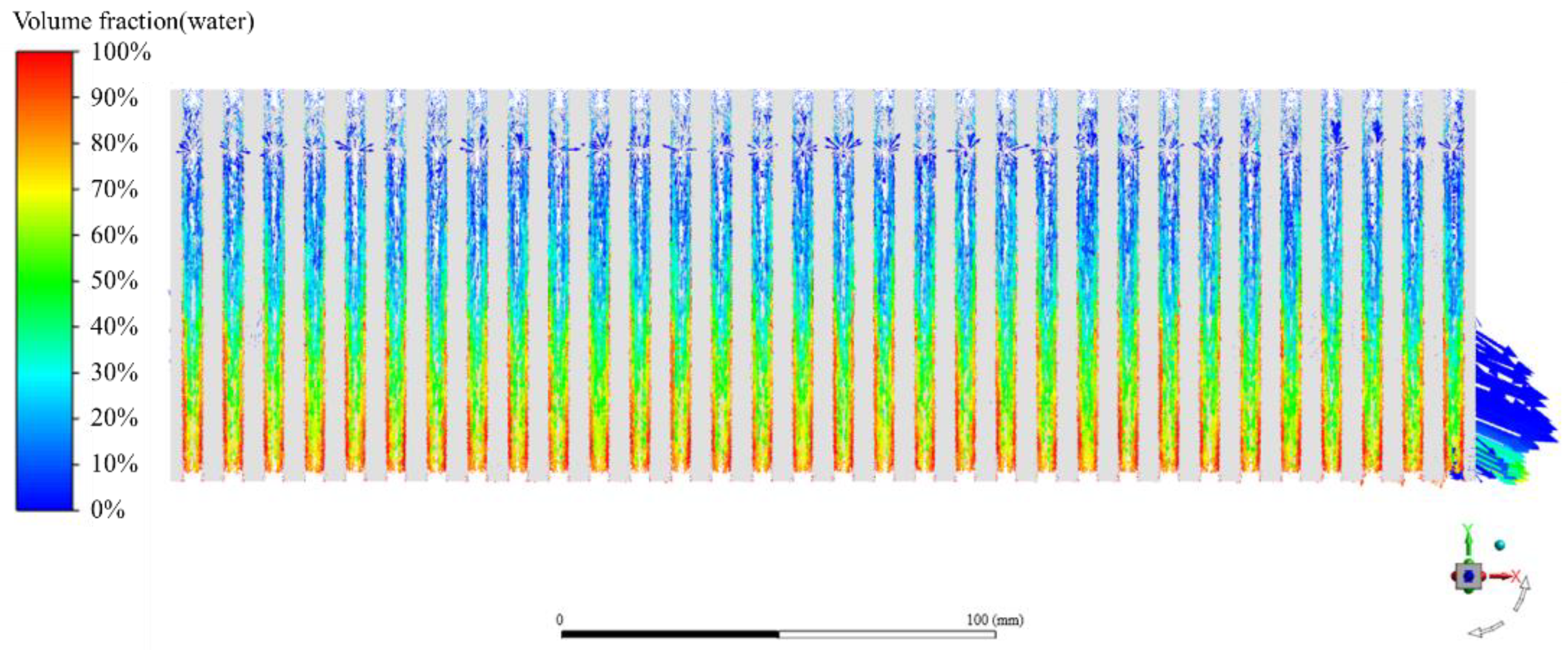
3.2. The Effect of the Geometric Parameters of the Corrugated Pipe on the Flow Field around the Pipe

Generally, the water supply conditions of field drainpipes include surface water infiltration supplies such as ponding water or rainfall or irrigation and lateral water supplies such as rivers. To simulate the real water supply situation and to further investigate the impact of perforation location on hydraulic characteristics during subsurface drainage, two other CFD models of subsurface drainage were established to simulate surface water infiltration supply and lateral water supply.

Streamline plots, that is, lines of flow that are tangential to the flow vectors at each point, were computed from a static global flow field obtained by estimating the mean flow direction at each point in space. We plotted the streamlines during the drainage research at a steady state, and we also calculated the flow rate of the pipe outlet and all the perforations at the shoulder section. Under all three kinds of water supply conditions, the streamline characteristics and the perforation flow rate ratio are shown in Figure 11 and

Table 5. Outer volume water flow rates of three kinds of water supply conditions.

Treatments	The Outer Volume Water Flow Rate (mL/s)	The Shoulder Perforation Volume Water Rate (mL/s)	The Volume Water Flow Ratio of the Shoulder Perforation to the Pipe Outlet (%)
Bottom water supply	53.36	4.14	7.75
Surface water supply	65.24	7.87	12.07
Lateral water supply	67.96	4.52	6.65

. As seen from the figure, a small volume of water flows into the drainpipe through two pieces of perforation at the shoulder of the pipe and most of the water flows into the drainpipe through the perforation at the bottom of the pipe. Finally, the water was pooled at the bottom of the pipe and ultimately flowed out.

As seen from the distributions of the velocity vector of the volume fraction of water located in the corrugation valley plotted in Figure 12, the water flows from top to bottom along the wall of the corrugation valley of the pipe, and the volume fraction of water gradually increases from top to bottom.

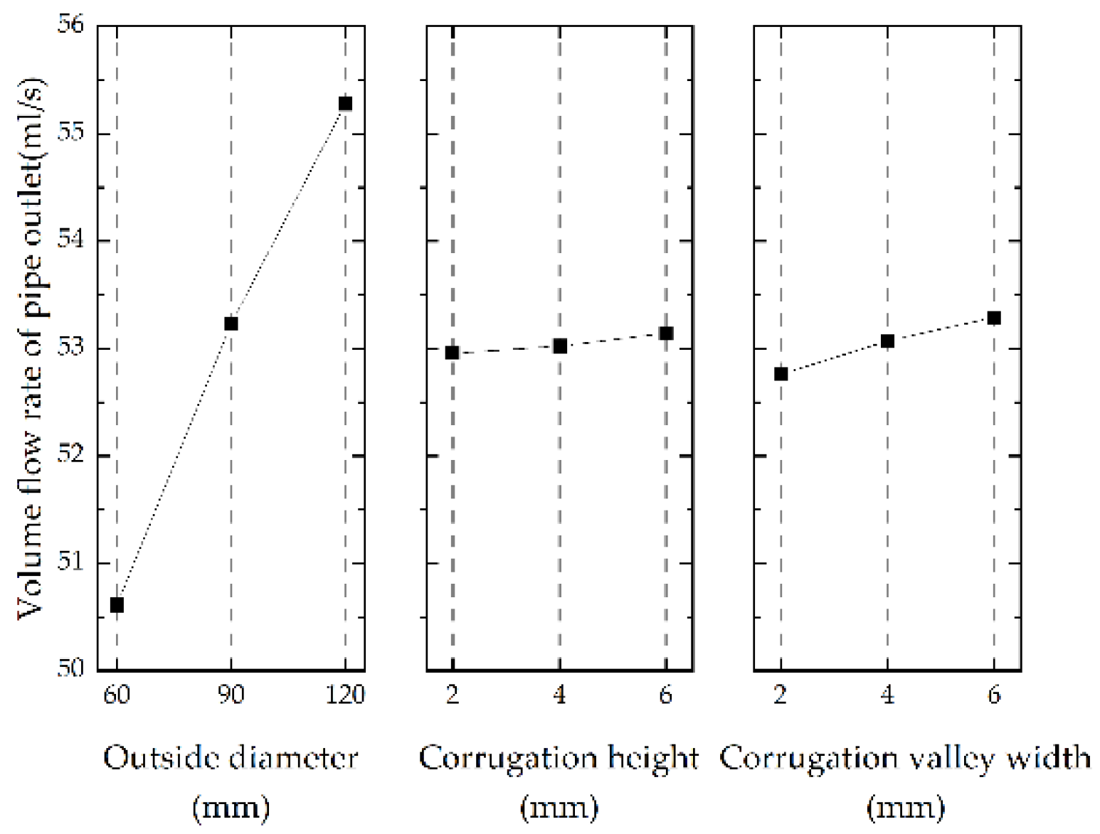
3.3. The Effect of the Geometric Structure of the Corrugated Pipe on the Drainage Rate

3.3.1. The Effect of the Corrugation Structure of the Corrugated Pipe on the Drainage Rate

To evaluate the relationship between the corrugation geometric structure and drainage rate more accurately, we designed an orthogonal test with factors including the outside diameter, corrugation height and corrugation valley width. The L₉(3⁴) orthogonal test adopted range analysis and variance analysis (ANOVA) of the orthogonal test to determine the interaction between the basic factors and minor factors.

The range analysis of the volume flow rate of the drainpipe is shown in

Table 6. Range analysis of the volume flow rate of the drainpipe.

Treatments	Factors				Outer Volume Flow Rate (mL/s)
	Factor A: Outside Diameter (mm)	Factor B: Corrugation Height (mm)	Factor C: Corrugation Valley Width (mm)	Blank
T1	60	2	2	1	50.31
T2	60	4	4	2	50.62
T3	60	6	6	3	50.91
T4	90	2	6	2	53.39
T5	90	4	2	3	52.88
T6	90	6	4	1	53.43
T7	120	2	4	3	55.17
T8	120	4	6	1	55.57
T9	120	6	2	2	55.09
k1	50.61	52.96	52.76	53.10
k2	53.23	53.02	53.07	53.03
k3	55.28	53.14	53.29	52.99
R	4.67	0.19	0.53	0.11
Factor order	A > C > B
Optimal level combination	A3B2C3

. The range analysis of orthogonal experiments showed that the sequence of the factors affecting the drainage was as follows: outside diameter, corrugation valley width and corrugation height. The trend analysis was drawn with the factors and levels of the orthogonal test as horizontal coordinates and the mean value of the indicator as the ordinate, as shown in Figure 13. The calculation indicated that when the trial protocol was set to A₃B₂C₃, in which the outside diameter was 120 mm, the corrugation height was 4 mm and the corrugation valley width was 6 mm, the maximal drainage flow was 55.57 mL/s, as shown in treatment 8 in Table 6.

The significant factors were determined from the experimental data by using ANOVA. The results are presented in

Table 7. ANOVA of the volume flow rate of the drainpipe.

Sources	Sum of Squares of Deviations	Degrees of Freedom	Mean Square	F	p-Value
Outside diameter	32.786	2	16.393	1584.729	0.001
Corrugation height	0.054	2	0.027	2.595	0.278
Corrugation valley width	0.426	2	0.213	20.592	0.046
Error	0.021	2	0.010
Combined errors	33.29

. The results indicated that outside diameter and corrugation valley width have a significant impact on drainage, corrugation height has small impacts and the outside diameter is the most critical influencing factor.

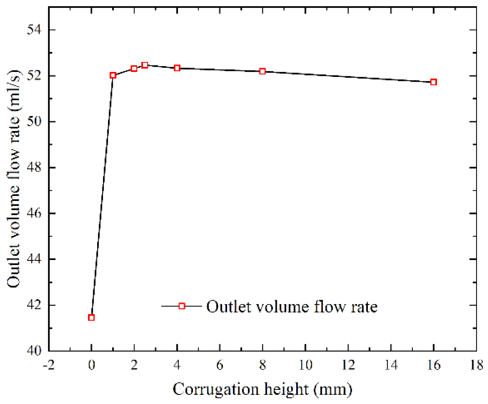
3.3.2. The Effect of Outside Diameter and Corrugation Height on Drainage Rate

Further analysis and quantification were performed using the CFD model. The outside diameter was set to 60 mm, 90 mm, 110 mm, 130 mm and 160 mm. All the boundary conditions and initial conditions remained unchanged. In all these treatments, the perforation area of the pipe was 51 cm²/m, and the distance between the inlet and the perforation at the bottom of the drainpipe was 400 mm. This ensures that the CFD model was calculated under identical conditions to guarantee identical pressure heads of the perforation at the bottom from different tests. The results showed that, under the same perforation area, the larger the outside diameter was, the larger the volume flow rate of the outlet. The results are plotted in Figure 14.

Similarly, for the same purpose, to analyze the corrugation height effects, the calculation was carried out under five different settings. The CFD models were established under the same outside diameter, and these corrugation heights were set as follows: 16 mm, 8 mm, 4 mm, 2.5 mm, 2 mm, 1 mm and zero (smooth). The results showed that the volume flow rate of the outlet of the corrugated pipe is 26% greater than that of the smooth pipe, but an increased corrugation height does not result in a greater volume flow rate of the outlet. The results are plotted in Figure 15.

4. Discussion

Through the analysis of the hydraulic characteristics of the flow field by the steady-state 3D subsurface drainage CFD model established in this study, we found that the water table forms an elliptical shape and that flow to the drain is driven by the slope (energy gradient) of the water table, which is consistent with Waller and Yitayew [35]. The flow lines are not always toward the drainpipe, as described in Ernst [9]. The flow toward the drain can be described by vertical and horizontal flow toward the vicinity of the drain and radial flow toward the drain and entry into the drain. In addition, from the streamline and the velocity vector of water in the immediate vicinity of the pipe, during the drainage process, the water flows into the corrugation valley, converges at the bottom of the corrugation valley and mainly enters the pipe through the bottom perforation, as shown in Figure 11 and Figure 12.

The existing theoretical calculation formulas that describe steady-state subsurface pipe drainage flow, such as the Hooghoudt equation, are based on the following assumptions: the drainpipes are half-full and the location where the water table and pipe intersect is the outside edge of the central elevation of the pipe [35,36]. However, hanging curtain drains are universally present during the processes of lowering groundwater tables in a subsurface drainage system, and there is a certain difference between the water table in the real drainage process of drainpipes and this assumption. Tao Yuan and Li Na [37] analyzed the applicability of the theoretical formula of drainage flow under the influence of soil texture and hanging curtain sections. This paper shows that different drainpipe structures will also affect the shape of the hanging curtain section, as shown in Figure 10. Cavelaars [10] indicated that the entrance resistance can be reduced through pipes with larger diameters. This study shows that increasing the outside diameter and corrugation valley width increases the contact face area between the corrugation valley and soil and increases the drainage flow rate; therefore, the water table in the immediate vicinity of the pipe decreases with soil water discharge.

Although the pipe outside diameter is positively correlated with the drainage performance, the drainage flow rate does not increase significantly with the pipe outside diameter. In addition, the manufacturing of larger diameter pipes requires more raw materials, which will lead to an increase in cost, but a larger diameter will not bring a significant increase in drainage performance. Therefore, the small diameter drainpipe has higher use efficiency and relatively low manufacturing cost, which is also more conducive to the promotion of farmland subsurface drainage technology.

5. Conclusions

In this paper, we propose a 3D steady-state subsurface drainage CFD model for subsurface drainage. The proposed model considers the geometric parameters of corrugated pipes and the water supply direction. The model established is calibrated as follows: First, the parameters of the numerical model are calibrated through the sand tank subsurface drainage experiment and the accuracy of the model is verified. Then, the hydraulic characteristics of the flow field in the steady-state subsurface drainage process under different subsurface geometries are described. Finally, based on the principle of orthogonal experimental design, the sensitivity of the outside diameter, corrugation valley width and corrugation height of the corrugated pipe to the drainage flow is analyzed. The main conclusions are as follows:

(1) A steady-state 3D subsurface drainage model can be established based on CFD technology. The drainage flow rate and water head pressure distribution characteristics calculated by the model are well-fitted to the sand tank subsurface drainage experiment data (R² = 0.99);

(2) The proposed model describes the water movement feature in the process of subsurface drainage. We found that the water in the area near the drainpipe collects in the outer gap of the corrugated pipe and mainly enters the pipe through the bottom perforation. The drainage flow rate increases with increasing outer diameter and corrugation valley width; thus, the water table head of the drainpipe decreases;

(3) Among the geometric structure parameters of the corrugated pipe, the primary and secondary factors affecting the drainage flow are the pipe outside diameter, corrugation valley width and corrugation height. Among them, the pipe outside diameter and the corrugation valley width have a significant impact on the drainage flow, with the outside diameter being the most critical influencing factor.

In this study, the subsurface drainage model integrates the hydraulic conductivity of envelope materials and soil on water infiltration. In addition, the model only considers steady-state underground drainage and ignores the dynamic drainage process. In the next step, it is necessary to consider the hydraulic conductivity of envelop materials and different soil textures and to further analyze the influence of the shape and pattern of the perforations on the drainage performance.

References

1. Gao, D.; Yang, H.; Yu, W.; Wu, X.; Wu, A.; Lu, G.; Zheng, Q. Research on the Mechanical Behavior of Buried Double-Wall Corrugated Pipes. Polymers 2022, 14, 4000. [Google Scholar] [CrossRef] [PubMed]
2. Yannopoulos, S.I.; Grismer, M.E.; Bali, K.M.; Angelakis, A.N. Evolution of the Materials and Methods Used for Subsurface Drainage of Agricultural Lands from Antiquity to the Present. Water 2020, 12, 1767. [Google Scholar] [CrossRef]
3. Valipour, M.; Krasilnikof, J.; Yannopoulos, S.; Kumar, R.; Deng, J.; Roccaro, P.; Mays, L.; Grismer, M.E.; Angelakis, A.N. The Evolution of Agricultural Drainage from the Earliest Times to the Present. Sustainability 2020, 12, 416. [Google Scholar] [CrossRef] [Green Version]
4. Stuyt, L.C.P.M.; Dierickx, W.; Beltrán, J.M. Materials for Subsurface Land Drainage Systems; Food and Agriculture Organization: Rome, Italy, 2005. [Google Scholar]
5. Oyarce, P.; Gurovich, L.; Duarte, V. Experimental Evaluation of Agricultural Drains. J. Irrig. Drain. Eng. 2017, 143, 04016082. [Google Scholar] [CrossRef]
6. Stuyt, L.; Dierickx, W. Design and performance of materials for subsurface drainage systems in agriculture. Agric. Water Manag. 2006, 86, 50–59. [Google Scholar] [CrossRef]
7. Alavi, S.A.; Naseri, A.A.; Bazaz, A.; Ritzema, H.; Hellegers, P. Performance evaluation of the Hydroluis drainpipe-envelope system in a saline-sodic soil. Agric. Water Manag. 2020, 243, 106486. [Google Scholar] [CrossRef]
8. Li, H.; Wu, Z.; Yang, H.; Wu, J.; Guo, C. Field study on the influence of subsurface drainage pipes and envelopes on discharge and salt leaching in arid areas. Irrig. Drain. 2022, 71, 697–710. [Google Scholar] [CrossRef]
9. Ernst, L.F. HET Berekenen van Stationnaire Grondwaterstromingen, Welke in Een Verticaal Vlak Afgebeeld Kunnen Worden; Landbouwproefstation en Bodemkundig Instituut TNO: Groningen, The Netherlands, 1954. [Google Scholar]
10. Cavelaars, J. Problems of Water Entry into Plastic and Other Drain Tubes; National College of Agricultural Engineering: Bedfordshire, UK, 1967. [Google Scholar]
11. Childs, E.C.; Youngs, E.G. The nature of the drain channel as a factor in the design of a land-drainage system. Eur. J. Soil Sci. 1958, 9, 316–331. [Google Scholar] [CrossRef]
12. Dierickx, W. Research and developments in selecting subsurface drainage materials. Irrig. Drain. Syst. 1993, 6, 291–310. [Google Scholar] [CrossRef]
13. Smedema, L.K.; Rycroft, D.W. Land drainage. Planning and design of agricultural drainage systems. Agric. Water Manag. 1983, 10, 183–184. [Google Scholar]
14. Bahçeci, I.; Nacar, A.S.; Topalhasan, L.; Tari, A.F.; Ritzema, H.P. A New Drainpipe-Envelope Concept for Subsurface Drainage Systems in Irrigated Agriculture. Irrig. Drain. 2018, 67, 40–50. [Google Scholar] [CrossRef]
15. Gaj, N.; Madramootoo, C.A. Effects of Perforation Geometry on Pipe Drainage in Agricultural Lands. J. Irrig. Drain. Eng. 2020, 146, 04020015. [Google Scholar] [CrossRef]
16. Wesseling, J.; Homma, F. Entrance resistance of plastic drain tubes. Neth. J. Agric. Sci. 1967, 15, 170–182. [Google Scholar] [CrossRef]
17. Šimůnek, J.; van Genuchten, M.T.; Šejna, M. The HYDRUS Software Package for Simulating Two-and Three-Dimensional Movement of Water, Heat, and Multiple Solutes in Variably-Saturated Media; Technical Manual, Version 2.0; University of California Riverside: Riverside, CA, USA, 2006. [Google Scholar]
18. Skaggs, R.W.; Youssef, M.A.; Chescheir, G.M. DRAINMOD: Model Use, Calibration, and Validation. Trans. Asabe 2012, 55, 1509–1522. [Google Scholar] [CrossRef]
19. Kroes, J.G.; Van Dam, J.C.; Huygen, J.; Vervoort, R.W. User’s Guide of SWAP Version 2.0; Simulation of Water Flow, Solute Transport and Plant Growth in the Soil-Water-Atmosphere-Plant Environment; Technical Document; Altera: Denver, CO, USA, 1999. [Google Scholar]
20. Kroes, J.; Wesseling, J.; van Dam, J. Integrated modelling of the soil–water–atmosphere–plant system using the model SWAP 2· 0 an overview of theory and an application. Hydrol. Process. 2000, 14, 1993–2002. [Google Scholar] [CrossRef]
21. Li, X.; Zuo, Q.; Shi, J.; Wang, S.; Bengal, A. Evaluation of salt discharge by subsurface pipes in the cotton field with film mulched drip irrigation in Xinjiang, China II: Application of the calibrated models and parameters. J. Hydraul. Eng. 2016, 47, 616–625. [Google Scholar]
22. Shaoli, W.; Xingkui, W.; Prasher, S. Field application of DRAINMOD model to the simulation of water table, surface runoff and subsurface drainage. Trans. Chin. Soc. Agric. Eng. 2006, 22, 54–59. [Google Scholar]
23. Filipović, V.; Mallmann, F.J.K.; Coquet, Y.; Šimůnek, J. Numerical simulation of water flow in tile and mole drainage systems. Agric. Water Manag. 2014, 146, 105–114. [Google Scholar] [CrossRef] [Green Version]
24. Boivin, A.; Šimůnek, J.; Schiavon, M.; Genuchten, M.T. Comparison of Pesticide Transport Processes in Three Tile-Drained Field Soils Using HYDRUS-2D. Vadose Zone J. 2006, 5, 838–849. [Google Scholar] [CrossRef] [Green Version]
25. Tao, Y.; Wang, S.; Xu, D.; Yuan, H.; Chen, H. Field and numerical experiment of an improved subsurface drainage system in Huaibei plain. Agric. Water Manag. 2017, 194, 24–32. [Google Scholar] [CrossRef]
26. Li, X.W.; Zuo, Q.; Shi, J.C.; Alon, B.; Wang, S. Evaluation of salt discharge by subsurface pipes in the cotton field with film mulched drip irrigation in Xinjiang, China I. Calibration to models and parameters. J. Hydraul. 2016, 47, 537–544. [Google Scholar]
27. Hirsch, C. Numerical Computation of Internal and External Flows. Int. J. Heat Fluid Flow 2007, 10, 371. [Google Scholar]
28. Lee, I.-B.; Bitog, J.P.P.; Hong, S.-W.; Seo, I.-H.; Kwon, K.-S.; Bartzanas, T.; Kacira, M. The past, present and future of CFD for agro-environmental applications. Comput. Electron. Agric. 2013, 93, 168–183. [Google Scholar] [CrossRef]
29. Afrin, T.; Khan, A.A.; Kaye, N.B.; Testik, F.Y. Numerical Model for the Hydraulic Performance of Perforated Pipe Underdrains Surrounded by Loose Aggregate. J. Hydraul. Eng. 2016, 142, 04016018. [Google Scholar] [CrossRef]
30. Fu, H.; Yang, L.; Liang, H.; Wang, S.; Ling, K. Diagnosis of the single leakage in the fluid pipeline through experimental study and CFD simulation. J. Pet. Sci. Eng. 2020, 193, 107437. [Google Scholar] [CrossRef]
31. Tu, J.; Yeoh, G.H.; Liu, C. Computational Fluid Dynamics: A Practical Approach; Butterworth-Heinemann: Oxford, UK, 2018. [Google Scholar]
32. Hirt, C.W.; Nichols, B.D. Volume of fluid (VOF) method for the dynamics of free boundaries. J. Comput. Phys. 1981, 39, 201–225. [Google Scholar] [CrossRef]
33. Forchheimer, P. Wasserbewegung Durch Boden: Zeitschrift des Vereines Deutscher Ingenieure; Eitschrift des Vereins Deutscher Ingenieure: Düsseldorf, Germany, 1901. [Google Scholar]
34. Darcy, H. Les Fontaines Publiques de la ville de Dijon: Exposition et Application des Principes à Suivre et des Formules à Employer dans les Questions de Distribution D’eau: Ouvrage Terminé par un Appendice Relatif aux Fournitures D’eau de plusieurs Villes, au Filtrage des Eaux et à la Fabrication des Tuyaux de Fonte, de Plomb, de Tôle et de Bitume; Dalmont, V., Ed.; Ghent University: Ghent, Belgium, 1856; Volume 2. [Google Scholar]
35. Waller, P.; Yitayew, M. Irrigation and Drainage Engineering; Springer: New York, NY, USA, 2016. [Google Scholar]
36. Ritzema, H.P. Drainage Principles and Applications; International Institute for Land Reclamation and Improvement: Wageningen, The Netherlands, 1994. [Google Scholar]
37. Yuan, Y.; Na, L.; Shaoli, W. Discussion on the formula of subsurface drainage discharge considering hanging curtain section. Trans. Chin. Soc. Agric. Eng. 2021, 37, 119–126. [Google Scholar]
Figure 1. Technological road map of this study.
Agriculture 12 02174 g001
Figure 2. Schematic representation of the sand tank experiment.
Agriculture 12 02174 g002
Figure 3. Particle size distribution of the test soil.
Agriculture 12 02174 g003
Figure 4. Sketch of the subsurface drainage corrugated pipe. k = corrugation height; c = corrugation pitch; j = corrugation valley width.
Agriculture 12 02174 g004
Figure 5. Schematic of the model and boundary conditions.
Agriculture 12 02174 g005
Figure 6. Mesh model.
Agriculture 12 02174 g006
Figure 7. Plot of the water head horizontally along the pipe for different mesh sizes.
Agriculture 12 02174 g007
Figure 8. Corrugated pipe numerical model of the orthogonal test. (A: outer diameter; B: groove depth; C: groove width).
Agriculture 12 02174 g008
Figure 9. Distribution profiles.
Agriculture 12 02174 g009
Figure 10. Soil water content of the pipe outside diameter (mm) = (a) 60 mm, (b) 90 mm and (c) 120 mm.
Agriculture 12 02174 g010
Figure 11. Streamlines with the velocity magnitude (m/s) for the global–local flow field.
Agriculture 12 02174 g011
Figure 12. Velocity vectors near the wall of the corrugated pipe.
Agriculture 12 02174 g012
Figure 13. Relationships between the volume flow rate of the pipe outlet and factors.
Agriculture 12 02174 g013
Figure 14. Relationship between the volume flow rate and outside diameter.
Agriculture 12 02174 g014
Figure 15. Relationship between the volume flow rate and corrugation height.
Agriculture 12 02174 g015