Article

Forecasting Agricultural Commodity Prices Using Dual Input Attention LSTM

1
Department of Computer Science and Engineering, Sejong University, Seoul 05006, Korea
2
Department of Convergence Engineering for Intelligent Drone, Sejong University, Seoul 05006, Korea
*
Author to whom correspondence should be addressed.
These authors contributed equally to this work.
Agriculture 2022, 12(2), 256; https://doi.org/10.3390/agriculture12020256
Submission received: 11 January 2022 / Revised: 31 January 2022 / Accepted: 7 February 2022 / Published: 10 February 2022
(This article belongs to the Section Agricultural Economics, Policies and Rural Management)

Abstract

:
Fluctuations in agricultural commodity prices affect the supply and demand of agricultural commodities and have a significant impact on consumers. Accurate prediction of agricultural commodity prices would facilitate the reduction of risk caused by price fluctuations. This paper proposes a model called the dual input attention long short-term memory (DIA-LSTM) for the efficient prediction of agricultural commodity prices. DIA-LSTM is trained using various variables that affect the price of agricultural commodities, such as meteorological data, and trading volume data, and can identify the feature correlation and temporal relationships of multivariate time series input data. Further, whereas conventional models predominantly focus on the static main production area (which is selected for each agricultural commodity beforehand based on statistical data), DIA-LSTM utilizes the dynamic main production area (which is selected based on the production of agricultural commodities in each region). To evaluate DIA-LSTM, it was applied to the monthly price prediction of cabbage and radish in the South Korean market. Using meteorological information for the dynamic main production area, it achieved 2.8% to 5.5% lower mean absolute percentage error (MAPE) than that of the conventional model that uses meteorological information for the static main production area. Furthermore, it achieved 1.41% to 4.26% lower MAPE than that of benchmark models. Thus, it provides a new idea for agricultural commodity price forecasting and has the potential to stabilize the supply and demand of agricultural products.

1. Introduction

Agricultural commodities play a significant role in the daily lives of people. Fluctuations in agricultural commodity prices can burden consumers and cause instability in farm household income. The abnormal climate in recent years has further aggravated fluctuations in agricultural commodity prices, making it difficult for governments to develop policies and make decisions to stabilize supply and demand [1]. The Ministry of Agriculture, Food and Rural Affairs (MAFRA), in South Korea, has been endeavoring to manage supply and demand to ensure the stability of price and farm household income by designating cabbage, radish, onion, garlic, and hot peppers grown in the field as “five vegetables sensitive to supply and demand”. Stabilizing the supply and demand of agricultural commodities is difficult. However, by providing more accurate price forecasts for agricultural commodities, it is possible to reduce the risk caused by price fluctuations and ultimately achieve this goal [2].
Meteorological factors have a direct impact on agricultural production and, hence, meteorological information is essential for the prediction of agricultural commodity prices [3]. Agricultural commodities grown in the open field are more affected by meteorological conditions than those grown in facilities, such as greenhouses. As the “five vegetables sensitive to supply and demand” are mainly grown in open fields, their yields are more susceptible to meteorological conditions [2,4], which can further affect their supply and price [5].
Various studies have been conducted with the objective of predicting agricultural commodity prices [6,7,8,9,10]. However, only a few [11,12] used meteorological data. For example, Jin et al. [12] predicted the price of cabbage and radish grown in the open field using meteorological data. Yin et al. [11] used eight types of meteorological data, including average temperature and accumulated precipitation, to predict the price of the “five vegetables sensitive to supply and demand”. However, in these studies, meteorological information from the static main production area was used.
A static main production area is a main production area for each agricultural commodity selected in advance based on statistical data. The selected main production area does not change until the next statistical data are released. However, the main production area for agricultural commodities grown in the open field may change annually owing to climate change, and the agricultural commodities may have different production periods owing to differences in local meteorological conditions. In addition, because the statistical data used are generally provided yearly, it is difficult to accurately determine the production period of agricultural commodities; and it is not possible to explain the main production area of agricultural commodities for each period. To solve this problem, this study uses meteorological information from the dynamic main production area. A dynamic main production area is a main production area dynamically selected based on the production of agricultural commodities in each region. The method of dynamically selecting the main production area is described in detail in Section 2.1.3.
Existing research related to agricultural commodity prices forecast is divided into two types: statistical methods and intelligent methods. The autoregressive integrated moving average (ARIMA) and the seasonal autoregressive integrated moving average (SARIMA) models are the most widely used statistical methods for time series prediction. Darekar and Reddy [13] used the ARIMA model to predict cotton prices in major cotton-producing regions in India. Jadhav et al. [14] used the ARIMA model to predict the prices of rice, finger millets, and maize in Karnataka, India, and Pardhi et al. [15] used the ARIMA model to predict the price of mango. Assis et al. [16] predicted cocoa bean prices using a combination of ARIMA and generalized autoregressive conditional heteroskedasticity (GARCH), which outperformed ARIMA. Unlike the ARIMA model, which is based on the difference operator, the SARIMA model is based on the seasonal difference operator. This converts non-stationary time series data into wide-sense stationary time series data by removing not only the trend component but also the seasonal component [17]. For this reason, the SARIMA model has been widely used to predict the price of agricultural commodities with strong seasonality. Adanacioglu and Yercan developed a SARIMA model to predict the wholesale price of tomatoes in Turkey and analyze seasonal fluctuations in tomato prices [6]. In addition to tomato price prediction, the SARIMA model was used to predict the prices of agricultural commodities, such as potatoes, onions, and jackfruit [18,19,20]. In addition to the ARIMA and SARIMA models, various statistical methods, such as Holt Winter’s model, linear regression (Balaji Prabhu and Dakshayini [21]), and multivariate regression model [22], were used to predict agricultural commodity prices. Because statistical methods, such as ARIMA and SARIMA, are based on a linear assumption, the performance of the built model may be very poor when predicting time series data with strong nonlinearity [1].
Intelligent methods, such as artificial neural networks (ANN) and recurrent neural networks (RNN), have also been used to predict agricultural prices. Zhang and Qi [23] and Zhang and Kline [24] utilized artificial neural networks in time series data with high seasonality, and, in fact, machine learning and deep learning-based algorithms, including artificial neural networks, have been recognized as efficient approaches for solving time series prediction problems. Wei et al. [7] and Weng et al. [25] show the superiority of the approach using artificial neural networks compared to statistical methods in predicting agricultural prices. Wei et al. [7] performed price forecasting for various agricultural commodities using a backpropagation neural network (BPNN). They proved that the improved BPNN model is an efficient method to predict agricultural commodity prices by comparing the proposed model to the statistical model. Weng et al. [25] conducted a study to predict the price of horticultural products. In a monthly, weekly, and daily average price forecasting, the neural network recorded higher performance than the ARIMA model. Li et al. [26] conducted a study to predict the weekly retail price of eggs in the Chinese market by proposing a chaotic neural network. The performance of the chaotic neural network and ARIMA was compared, and the chaotic neural network recorded better nonlinear fitting ability and higher prediction precision in the weekly retail price of eggs. Hemageetha and Nasira [8] predicted tomato prices using a BPNN and a radial basis function neural network (RBF), which proved the superiority of the RBF model through experiments. Another type of ANN called the extreme learning machine (ELM) [27] has been applied to predict the price of agricultural commodities using various techniques. Wang et al. [28] predicted the price of corn using a hybrid model that combined the singular spectrum analysis (SSA) method and ELM. This shows that the proposed method can improve the accuracy of forecasting by better understanding the overall trend of price changes.
ANNs have limitations in modeling sequential data because they handle input data points independently without considering the correlation among input data. Because the agricultural commodity prices to be predicted in this study are time series data, it is important to model the time series characteristics of the price data. RNN specializing in learning sequential data can be trained with time series information of data through its internal cyclic structure. Long short-term memory (LSTM), a type of RNN, is considered one of the most popular methods for dealing with time series prediction problems. Shin et al. [9] used LSTM to predict the price of green onion, onion, zucchini, rice, and spinach. In their study, a predictive model was trained using various variables that affect the price of agricultural commodities, such as weather data, the rate of price increase of agricultural commodities, the previous year’s yield of agricultural commodities, and the area cultivated in the previous year. They reported that their method exhibited better performance than previous time series prediction models. Jin et al. [12] predicted the price of cabbage and radish by using an STL-LSTM model that combines the STL technique and the LSTM model. The STL technique was used to solve the high seasonality of agricultural commodity price data and the “lag” phenomenon that appears in the prediction results. They reported MAPEs of approximately 7.95% and 11.25% for the price predictions of cabbage and radish, respectively.
The attention mechanism introduced in neural machine translation has the advantage of overcoming the long-term dependency and information loss of RNNs, which enables better characterization of the input data by assigning different importance to each element of the input sequence and paying attention to the more relevant input [29]. Currently, the attention mechanism is widely used in fields, such as natural language processing and computer vision, with recent attempts being made to apply it to time series prediction in various ways. In previous studies [30,31,32], different attention-based LSTM models were proposed and applied to travel time, financial time series, and temperature prediction. Yin et al. [11] applied the STL method and the attention-based LSTM model to predict the price of five agricultural commodities: cabbage, radish, onion, pepper, and garlic. However, previous studies have a common limitation of ignoring the dependency between time series data and the time series of data. To compensate for this problem, Qin et al. [33] proposed a dual-stage attention-based recurrent neural network (DA-RNN). Their proposed model could adaptively select the most relevant input features through the input and temporal attention mechanism, as well as learn the long-term temporal dependencies of the time series well. Liu et al. [34] proposed a dual-stage two-phase-based recurrent neural network (DSTP-RNN) to identify spatial correlations and temporal relationships.
Both the DA-RNN and DSTP-RNN models, which use the dual attention mechanism, have an encoder-decoder structure, and, instead of applying feature and temporal attention to the input at the same time, attention is applied to the input and context vector. No published study has reported application of the dual attention mechanism to agricultural commodity price prediction. This study incorporates the feature attention layer and temporal attention layer, which were designed to identify feature correlations and temporal relationships of the input data. Three previous studies used price and meteorological data as input variables [9,11,12], and this directly affected the growth of agricultural commodities. However, those studies only considered the meteorological information of the main production area to a limited extent. In this study, a dynamic main production area selection method was developed to determine the effects of meteorological conditions more accurately.
The contributions of this study are as follows. (1) Price, data, trading volume data, and meteorological data, which are rarely used in previous studies because they are difficult to handle, are used as input variables. (2) A dual input attention LSTM (DIA-LSTM), that concurrently applies feature and temporal attention, an upgraded version of the existing sequentially applied dual attention mechanism, is proposed. The proposed model is shown to provide 1.41% to 4.26% higher performance than benchmark models. (3) Considering the real situation, the meteorological information for the dynamic main production area is used. The performance of the model using the meteorological information for the dynamic main production area is shown to be an improvement of approximately 2.8 to 5.5% compared to the conventional model using the meteorological information for the static main production area.
The remainder of this paper is organized as follows. Section 2 introduces the proposed dual attention LSTM after explaining the data used in this study. Section 3 describes the performance metrics used in the experiment and discusses the experimental design and results. Finally, Section 4 presents the conclusions of this study and future research directions.

2. Materials and Methods

2.1. Dataset Description

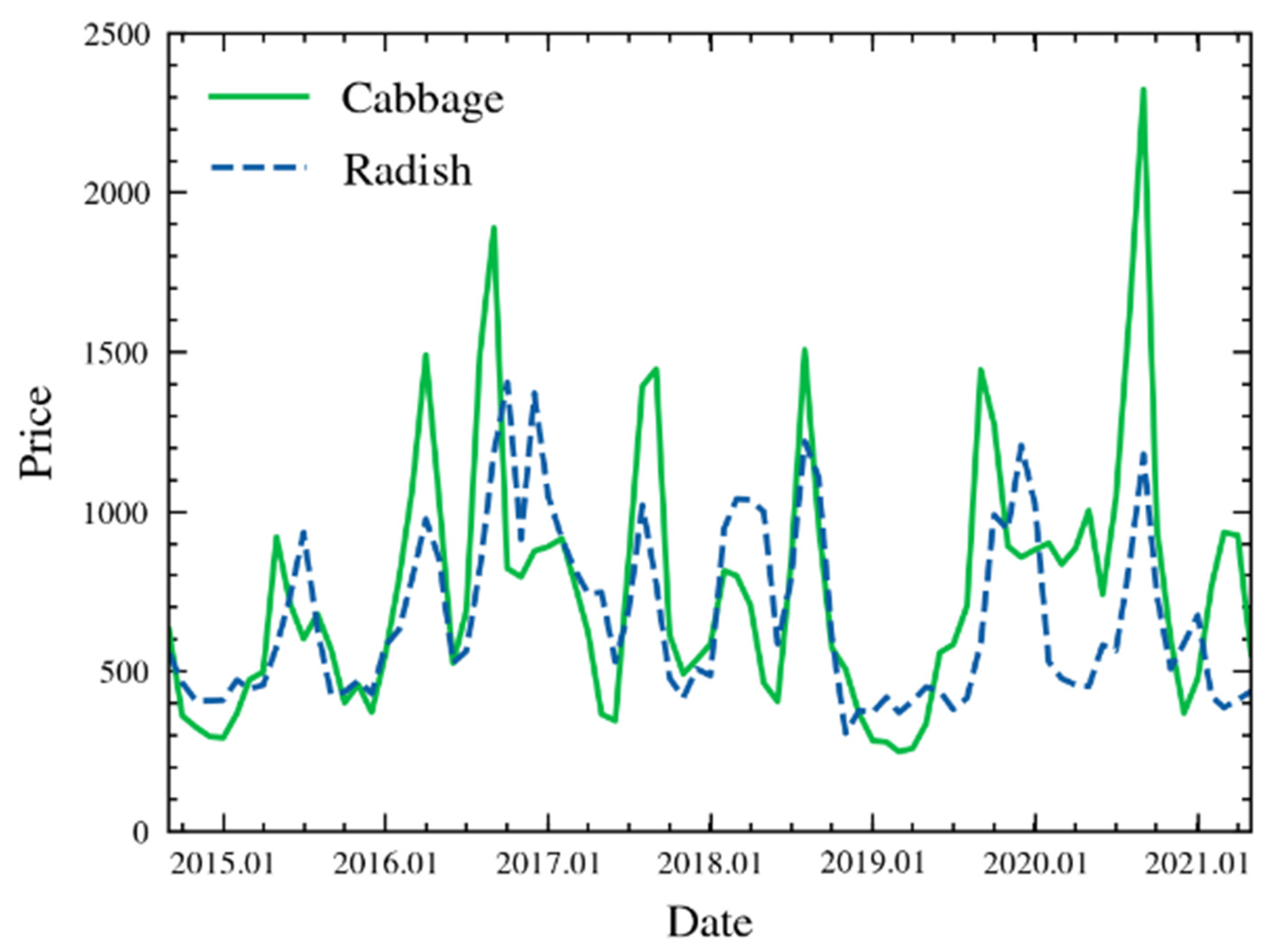
2.1.1. Wholesale Price of Agricultural Products

The data for the prices of cabbage and radish were downloaded from the Outlook & Agricultural Statistics Information System (OASIS) [35], provided by the Korea Rural Economic Institute (KREI) and Korea Agricultural Marketing Information Service (KAMIS), as well as by the Korea Agro-Fisheries & Food Trade Corporation (aT) [36]. OASIS and KAMIS provide daily prices for cabbage and radish. To predict the monthly average price, this study calculated and used the average value of the monthly grouped prices. The changes in the average monthly price of cabbage and radish are shown in Figure 1, indicating unstable fluctuations in the price. The average price of the previous month, exponential moving average (EMA), relative strength index (RSI), Williams %R, and median price, used as investment indicators, were used as derived variables.
Among them, the average price means the average value of the remaining three prices after removing the highest and lowest prices from the month’s price for the last five years. The open and close values used to calculate Williams %R were the prices on the first and last days of each month.

2.1.2. Trading Volume of Agricultural Products

The price of agricultural commodities is affected by the yield. Although it is desirable to use the yield of agricultural commodities as an input variable for the prediction model, it is difficult to apply the production data to the monthly price prediction because the statistics on production are published annually. Therefore, in this study, the trading volume of agricultural commodities was used instead of the yield. The agricultural products distribution system (NongNet) of aT provides daily trading volumes from each wholesale market.
In this study, the trading volume data provided by NongNet were divided into the national wholesale market, Garak market, and top five local market trading volumes. The national wholesale market trading volume is the sum of all wholesale markets. The Garak and top five local market trading volumes refer to the quantity brought in from a specific wholesale market. Among the numerous wholesale markets nationwide, the Garak and top five local markets play an important role in the daily lives of ordinary people and the distribution of agricultural and fishery products. Therefore, in this study, the Garak and the top five local market trading volumes were separately extracted and used as input variables for the model. Garak market is a wholesale market for agricultural and marine commodities located in Garak-dong (Songpa-gu, Seoul, Korea), and the Garak market trading volume refers to the quantity of agricultural and marine commodities brought into Garak market. The top five local markets refer to the wholesale markets for agricultural and marine commodities in Eomgung-dong, Busan; Gakhwa-dong, Gwangju; Guwol-dong, Incheon; Buk-gu, Daegu; and Ojeong-dong, Daejeon. The trading volume from the top five local markets is equal to the sum of the trading volumes from the aforementioned five wholesale markets. The daily data on the trading volumes of cabbage and radish were grouped monthly, and the sum was calculated and used.

2.1.3. Meteorological Data

Because cabbages and radishes are mainly grown in open fields, their yields are greatly affected by meteorological conditions [2]. Changes in the yield also affect changes in the price. Therefore, in this study, meteorological data provided by the Korean Meteorological Administration (KMA) was used as an input variable for the model. Meteorological indicators used include average temperature and humidity, accumulated precipitation, and typhoon advisory and warning in the main production area. Typhoon advisories and warnings have binary values indicating whether or not they are issued. The day typhoon advisories and warnings are issued is marked as 1, and a value counting the number of occurrences per month was used.
Meteorological data are generally provided by region; however, it is difficult to use all of this data in practice. Not all meteorological conditions in all regions affect the cultivation of specific agricultural commodities. In this study, the meteorological conditions of the main production area, where cabbages and radishes were grown, were examined. To use the meteorological data of the main production areas, it is necessary to know where the main production areas for each agricultural commodity are located. Although the Korean Statistical Information Service (KOSIS) [37] provides information on the main production areas of agricultural commodities every year, it is difficult to explain the main production areas that change according to the seasons because the data are provided annually. In the previous study [11], the main production area of agricultural commodities by harvest time provided by aT was used. In this method, different main production areas were used for each cropping season, but the same main production area is applied to the same cropping season in different years. Using this method, the selected main production area can be defined as a static main production area. However, the main production area may change slightly over time owing to climate change or urban development. To solve this problem, this study proposes a method for selecting a dynamic main production area. An area with a high yield based on its monthly yield, where agricultural commodities are grown, is selected as the dynamic main production area. In this study, the three regions with the highest yields were selected as the main production areas based on the yield a year back. Table 1 shows the main production areas of radish in July–September 2015, when the static and dynamic main production areas selection method were used.
Data were collected from September 2013 to May 2021 for the price, trading volume, and weather. Among them, data from September 2014 to January 2021 based on price were used as training data, and the remaining data from February 2021 to May 2021 were used as test data. Fixed data sizes were used for model training. Specifically, data from September 2014 to December 2020 were used as input data, and data up to January 2021 were used as target data. Data were forecasted a month ahead for testing the model by using actual observed past data. For example, to predict the price in February 2021, real data from previous months, such as January 2021, December 2020, etc., were used as inputs to the model. To predict the price during March 2021, the observed real data up until February 2021 were used as inputs to the model. The number of months of past data used to predict future prices depended on the hyperparameter of the time step.

2.2. Proposed Dual Input Attention LSTM (DIA-LSTM)

The dual input attention LSTM (DIA-LSTM) model proposed in this study predicts the price of the next month using various variables that affect agricultural commodity prices. The n variables that affect the price of agricultural commodities can be expressed as I = ( x 1 , x 2 , , x n ) , where x n means the time series for the n -th variable that affects the price. That is, X = ( x 1 , x 2 , , x T ) n × T , where T is the length of the time step (or window size). That is, the price of the next month is predicted using data from the past T months. The k -th input variable whose time step is T is expressed as x k = ( x 1 k , x 2 k , , x T k ) T , and the values of n input variables at time t is expressed as x t = ( x t 1 , x t 2 , , x t n ) n . The DIA-LSTM model uses the price of past agricultural commodities, y = ( y 1 , y 2 , , y T ) , with y t and past values of n input variables, ( x 1 , x 2 , , x T ) with x t n , to predict the price value of the next time step. For instance, next year, it will be y T + 1 . This is expressed in Equation (1), where means the proposed DIA-LSTM.
y ^ T + 1 = ( x 1 , x 2 , , x T , y 1 , y 2 , , y T ) .
DIA-LSTM consists of a feature attention layer, temporal attention layers, and a recurrent prediction layer. The structure is shown in Figure 2. The feature attention layer learns feature correlation in the input data X = ( x 1 , x 2 , , x t ) , and the temporal attention layer models the temporal relationship based on the transposed input data X = ( f 1 , f 2 , , f n ) . The output of the feature and temporal attention layer is generated by doing an element-wise multiplication (denoted by ) of the attention weights with the input data. The recurrent prediction layer predicts the final result value using the combined value of the output from the feature and temporal attention layers.
In previous studies, the dual attention mechanism was applied to the deep learning model of the encoder-decoder structure. Specifically, attention mechanisms were applied to the input and temporal axes in the encoder and decoder, respectively, and attention weights were calculated using LSTM and softmax. In this study, instead of using the encoder-decoder structure, a structure was used to input the input data into the LSTM model by concatenating the results of applying the attention mechanism to the input and temporal axes of the input data. In addition, a simple attention weight calculation method using a single linear layer and softmax was used. The difference between the structure of the existing dual attention mechanism and the proposed structure is shown in Figure 3. ( x 1 , x 2 , , x n ) denotes the inputs of the attention mechanism, and ( a 1 , a 2 , , a n ) is the attention weights obtained by the attention mechanism. The output can be generated by doing an element-wise multiplication (denoted by × ) of the attention weights with the inputs.
The feature attention layer (Appendix A.3) and temporal attention layer (Appendix A.4) were implemented by simplifying the single-layer perceptron. This was inspired by the self-attention mechanism (Appendix A.2) that can construct attention using only input values. Attention weights were applied to each input variable in the feature attention layer, as well as to each time step in the temporal attention layer.
The recurrent prediction layer consists of a single-layer stateful LSTM (Appendix A.1) and two fully connected layers (denoted by FC in Figure 2). The stateful LSTM model means that the hidden state h t learned in the current time step is transferred to the initial state during the next learning. The LSTM model receives the concatenation of the output X f of the feature attention layer and the output X t of the temporal attention layer. Subsequently, dropout is applied to the output of LSTM, and, after flattening (denoted by Flatten in Figure 2), it is input to the fully connected layer (FC). Table 2 shows the hyperparameter settings used in each layer. To predict the final single real value, the number of neurons in the last fully connected layer is set to 1.

2.3. Training Procedure

An Adam optimizer with a learning rate of 0.001 was used to train the model. To train the stateful LSTM, the size of the minibatch was set to 1, which was the highest common factor of the training and test data. Because DIA-LSTM is end-to-end differentiable, the parameters of the model can be learned through the backpropagation algorithm with the mean squared error as an objective function, as shown in Equation (2), where O means the objective function.
O ( y T + 1 , y ^ T + 1 ) = 1 N i = 1 N ( y ^ T + 1 i y T + 1 i ) 2 .
In Equation (2), N denotes the number of training samples, y ^ T + 1 i is the value predicted by DIA-LSTM, and y T + 1 i denotes the actual observed price value.

3. Results

This section describes the performance evaluation metrics used in the experiment and the experimental method to measure the performance of the proposed model. In this study, three experiments were conducted. The first experiment was to find the most suitable time step for the proposed DIA-LSTM model. The second experiment compares the performance of the model using meteorological data for the dynamic main production area and the model using meteorological data for the static main production area. The third experiment compares the performance of the DIA-LSTM model proposed in this study with the models proposed in other studies.

3.1. Evaluation Metrics

In this study, two different evaluation metrics were used to evaluate the performance of the model: root mean square error (RMSE) and mean absolute percentage error (MAPE). RMSE measures the difference between the real value and the predicted value. The definition is as follows:
RMSE = i = 1 N ( y ^ i y i ) 2 N .
MAPE is a widely used metrics in time series prediction and expresses the error between the real value and the predicted value as a percentage. The definition of MAPE is as follows:
MAPE = 1 N i = 1 N | y ^ i y i y i | × 100 % .
In Equations (3) and (4), N is the number of data samples, and y ^ i and y i are the real and predicted values of the i -th sample data, respectively. RMSE is obtained by subtracting the real value from the predicted value of each data sample. Subsequently, the average of the square values is calculated, and the root operation is performed. MAPE is obtained by calculating the absolute value after dividing the value obtained by subtracting the real value from the predicted value of each sample by the real value again. MAPE is more intuitive as it expresses the error as a percentage, regardless of the scale of the numbers it predicts.

3.2. Optimal Time-Step Search

In time series prediction, the time step is a hyperparameter that determines how many past data samples are used to predict future data; the optimal time step may differ depending on the task to be solved. In previous studies [11,32], several candidate values were set and a grid search was conducted to find the optimal time step. Different optimal time-step values were used for these studies. In this study, an experiment was conducted to find the most suitable time step for the data of two agricultural commodities (cabbage and radish).
In this experiment, the model was trained and performance was measured while changing the time step of the proposed DIA-LSTM. To find the optimal time step, a grid search was performed by setting the time step T { 1 ,   2 ,   4 ,   6 ,   8 ,   12 } . Table 3 shows the performance measurement results of the proposed model when the grid search was performed for time step T .
Consequently, both agricultural commodities recorded the lowest MAPE and RMSE when t = 6 . In a two-dimensional rectangular coordinate system, the graph was plotted with the x-axis as time step and the MAPE value as the y-axis, as shown in Figure 4. In the graph, both cabbage and radish had the lowest MAPE with t = 6 , and the error rate gradually increased when the time step became smaller or larger than t = 6 . This indicates that too small or large time steps in time series prediction can negatively affect model performance. If the time step is too small, it is difficult to learn sufficient information from past data. As the prediction is performed using only one data sample when t = 1 , the characteristics of the time series cannot be ascertained. Conversely, an increase in the MAPE with an increase in the time-step value may have been due to a decrease in the number of training data as the time-step value increased. This means that there were insufficient data to proceed with learning. In particular, because the size of the dataset used in the experiment was small, a large time step resulted in insufficiency in the training of the model.

3.3. Dynamic Main Production Area

To prove the superiority of the proposed dynamic main production area selection method, an experiment was conducted to compare the performance of a model using the meteorological data of the dynamic main production area, dynamically selected based on the yield, and a model using the predefined meteorological information of the main production area. The predefined main production area was adopted from a previous study [11], and all other data and parameter settings, except the main production area, were kept consistent. Table 4 shows the performance of the proposed model when the meteorological data of the dynamic and static main production areas are used.
For both cabbages and radishes, the model demonstrated higher performance when using the meteorological data of the dynamically selected main production area than that of the meteorological data of the predefined main production area. For cabbages, the MAPE when the dynamic main production area was used was 4.39%, which was approximately 5.51% lower than when the static main production area was used. For radishes, the MAPE when the dynamic main production area was used was 2.13%, which was improved by approximately 2.8% compared to when the static main production area was used.

3.4. Comparison with Benchmark Models

To verify the performance of the proposed model, various time series prediction models proposed in previous studies were selected as benchmark models, and an experiment was conducted to compare their performance. The benchmark models used for performance comparison are as follows.
Simple LSTM: The LSTM model proposed by Hochreiter and Schmidhuber [38] is often used for time series prediction owing its excellent long-term dependency learning ability. In this study, the part of the recurrent prediction layer that eliminated the feature and time attention layers from the DIA-LSTM model was used as a simple SLTM model.
GCN-LSTM: The GCN-LSTM model is based on the T-GCN model structure proposed by Zhao et al. [39]. T-GCN combines the graph convolutional layer [40] and the GRU model and has been applied to traffic prediction. In the GCN-LSTM used in this study, the GRU model of T-GCN was replaced with LSTM, and the dropout and density layers were added.
STL-ATTLSTM: The STL-ATTLSTM proposed by Yin et al. [11] is a model that combines the STL preprocessing technique and the attention mechanism-based LSTM model. The study predicts the prices of five crops, including cabbage and radish, using a variety of input variables.
DA-RNN: The DA-RNN model proposed by Qin et al. [33] is an encoder-decoder structure model, which consists of an encoder with an input attention mechanism applied and a decoder with a temporal attention mechanism. The proposed DA-RNN model recorded an impressive performance in indoor temperature prediction and stock price prediction.
Each model was tested using the same training and test datasets. Table 5 shows the results of measuring the performance of each model using RMSE and MAPE.
Table 5 shows the results of comparing the performance of the proposed DIA-LSTM model with the benchmark models. As shown in Table 5, the proposed DIA-LSTM model recorded the lowest RMSE and MAPE for cabbage and radish. Among the tested models, the average MAPE of simple LSTM was the highest, at 7.55%. This may have been due to the relatively simple LSTM model having weak learning ability compared to other benchmark models. Subsequently, GCN-LSTM recorded the second-highest error rate, with an average MAPE of 6.71%. Compared to the time series prediction method with the attention mechanism, the graph convolutional layer optimized for learning spatial information seems to have limitations in learning the characteristics of agricultural commodities with strong time series characteristics. STL-ATTLSTM and DSA-LSTM with an attention mechanism recorded an average MAPE of 4.67% and 4.90%, respectively. This is a lower error rate compared to the errors of simple LSTM and GCN-LSTM. Based on the results, the dual-stage attention-based model with the STL preprocessing technique and attention mechanism of STL-ATTLSTM, as well as the encoder with an input attention mechanism and a decoder with a temporal attention mechanism of DA-RNN, showed excellent performance. The reason for these results is that the attention mechanism used in the two studies can learn the time series characteristics of the input data and the characteristics of the input variables well. The DIA-LSTM model proposed in this study recorded the lowest error rate, of 3.26%. The model that combines the time and feature attention layers with LSTM was proven to be superior in solving the agricultural commodity price prediction problem.
Figure 5 shows the predicted value of the cabbage price for each model. The graph shows that the simple LSTM model has a large prediction error rate in March 2021 and April 2021, and the GCM-LSTM model has a large prediction error rate for the price in May 2021. STL-LSTM predicted all values smaller than the actual values, whereas DA-RNN predicted the price for the rest of the time steps with relatively high accuracy, except for the price for February 2021. Conversely, the proposed DIA-LSTM provided reliable predictions for all time steps. Figure 6 shows the predicted values of each model for the price of radish. LSTM showed a relatively large error rate in all forecasts, except for March 2021. GCN-LSTM was not stable, with large fluctuations in predicted values. DA-LSTM was able to predict the price of each time step relatively accurately, except for April 2021. Both the STL-LTM and the proposed DIA-LSTM could predict the price of radish relatively accurately.

4. Conclusions

This study introduces the feature and temporal attention layers that could capture feature correlations and temporal relationships for input variables, respectively, by applying the attention mechanism. Furthermore, a DIA-LSTM model combining two attention layers and an LSTM was proposed to predict the monthly price of cabbage and radish. The proposed model utilizes not only vegetable prices but also trading volumes from various markets, such as the national wholesale and top five local market trading volumes, and meteorological information for the main production areas. For the selection of the main production areas, the top three regions with high production volumes were dynamically selected as the main production areas, rather than using pre-defined static main production areas, as done by previous studies. Consequently, the performance of the model using the meteorological information of the dynamic main production area recorded approximately 5.51% and 2.8% lower error rates for cabbage and radish, respectively, than the model that uses predefined meteorological information of the static main production area. The proposed DIA-LSTM model averaged approximately 3.26% MAPE, with an error rate of approximately 1.41% to 4.26% lower than that of benchmark models.
Fluctuations in agricultural commodity prices affect the supply and demand of agricultural commodities and have a significant impact on consumers and farmers. Fluctuations in agricultural prices leads to uncertainty in the consumer’s daily consumption budget and income instability for the farmer. As a result of abnormal climate patterns, price fluctuations of agricultural products have intensified, making it difficult for the government to establish policies and stabilize supply and demand. The agricultural commodity price prediction model proposed in this study will help stabilize the supply and demand of agricultural products through more accurate predictions, thereby reducing the risk of price fluctuations.
The empirical results in this study are constrained by the lack of data and the fluctuation of prediction results. Monthly predictions about the agricultural commodity prices were made using data from September 2013 to May 2021, resulting in insufficient data to train a deep learning model. Sufficient price data can be collected from the 2000s, but the problem lies with the meteorological data, which are only available from 2012. Additional meteorological data should be obtained from the Meteorological Society or other agencies. The volume of data can also be increased by using weekly price forecasts instead of monthly forecasts. Although the prediction accuracy of the proposed model is relatively high, there are still large fluctuations between individual predictions. The stability of the model’s predictions can be improved by increasing the number of training variables that have an impact on prices, such as the export and import volumes of agricultural commodities.

Author Contributions

Conceptualization, Y.H.G., D.J. and H.Y.; methodology, Y.H.G. and D.J.; software, Y.H.G., D.J. and R.Z.; validation, Y.H.G., D.J. and X.P.; investigation, Y.H.G., D.J., R.Z. and X.P.; writing—original draft preparation, Y.H.G. and D.J.; writing—review and editing, Y.H.G., D.J. and H.Y.; supervision, Y.H.G., D.J. and S.J.Y.; project administration, S.J.Y. All authors have read and agreed to the published version of the manuscript.

Funding

This work was supported by an Institute of Information & Communications Technology Planning & Evaluation (IITP) grant funded by the Korea government (MSIT) (No. 2021-0-00755, Dark data analysis technology for data scale and accuracy improvement).

Institutional Review Board Statement

Not applicable.

Informed Consent Statement

Not applicable.

Data Availability Statement

Data is available from its original source as cited in the article. The wholesale price and trading volume data of agricultural products are available at KREI OASIS (https://oasis.krei.re.kr/index.do (accessed on 10 January 2022)) and aT KAMAS (https://www.kamis.or.kr/customer/main/main.do (accessed on 10 January 2022)) and the meteorological data is provided by Korean Meteorological Administration (https://data.kma.go.kr (accessed on 10 January 2022)).

Conflicts of Interest

The authors declare no conflict of interest.

Appendix A

Appendix A.1. LSTM Model

The LSTM proposed by Hochreiter et al. [38] constructs a recurrent neural network using a memory cell and three gates: output, forget, and input gates, efficiently solving the vanishing gradient problem that may occur during the training process of a simple recurrent neural network. The memory cell is a mechanism that exists in LSTM; its characteristic is that it flows only within the LSTM layer. The memory cell is denoted by c ; c t stores the memory of the LSTM at time t , and it stores necessary information from the past to time t . The forget gate tells which of the memory cells to “forget”, and the result is obtained through the calculation in Equation (A1).
f = sigmoid ( x t W x f + h t 1 W h f + b f ) .
As shown in Equation (A1), the input x t in the forget gate performs matrix multiplication with the weight W x f and the hidden state h t 1 of the previous time step with the weight W h f . The result f is obtained through the sigmoid function on the result of adding the two results and the bias b f of the forget gate. Considering that the sigmoid function converts the input to a value between zero and one, it acts as a gate by preserving more information in C t 1 when the value of f t is close to one, and by discarding more information from C t 1 when the value is close to zero. The superscript f of the weight W used here means a forget gate, and the subscripts x and h mean that the corresponding weight is an input, a hidden state, and a weight on which an operation is performed. The forget gate can erase the memory to be forgotten from the memory cell of the previous time step; however, it cannot decide which contents to remember. The gate that determines the information to be newly remembered is the input gate, which is defined by Equation (A3). The information to which the input gate that determines the information to be memorized is applied is calculated by Equation (A2).
g = tanh ( x t W x g + h t 1 W h g + b g ) ,
i = sigmoid ( x t W x i + h t 1 W h i + b i ) ,
c t = f c t 1 + g i .
The process of updating the memory cell by applying the forget and input gates is shown in Equation (A4), where means element-wise multiplication, and f c t 1 deletes the memory to be forgotten from the previous time step’s memory cell and adds new information to the memory cell through g i . By adding the two parts, we obtain the current time step’s memory cell c t .
The output gate adjusts the importance of each element in the next hidden state h t , where the output o of the output gate that determines the importance of each element is calculated by Equation (A5). The hidden state h t is the result of simply applying the tanh function to the memory cell c t , as shown in Equation (A6), and multiplying by element with the output o of the output gate.
o = sigmoid ( x t W x o + h t 1 W h o + b o ) ,
h t = o   tanh ( c t ) .

Appendix A.2. Attention Mechanism

The attention mechanism for sequence modeling was first introduced by Bahdanau et al. [29]. The rationale behind it is that, whenever the decoder predicts an output word, the encoder refers to the full input sentence once again. Instead of referring to all input sentences at the same ratio, the weight is raised on the word relevant to the word to be predicted at the moment to focus more on the word. There are several methods to calculate the weight; however, the method used by Bahdanau et al. [29] is as follows.
score ( s t , h i ) = v a tanh ( W a [ s t ; h i ] ) ,
α t , i = e x p ( score ( s t 1 , h i ) ) i = 1 n e x p ( score ( s t 1 , h i ) ) .
First, Equation (A7) is used to calculate the alignment score, where s t denotes the hidden state of the decoder, and t denotes the position of the output word as t = 1 ,   ,   m , with m representing the number of words in the output sentence. The alignment score can be calculated as a feed-forward network with a single hidden layer, enabling end-to-end training with other parts of the model. In the attention mechanism, the weights v a and W a are learned. Subsequently, the attention weight α t , i calculated by Equation (A8) means the alignment weight between the t -th output word and the i -th input word. An input with an attention weight applied can be obtained by applying such an attention mechanism to the input time series data. Using the attention mechanism, a layer that can model feature and temporal correlations for input data was introduced in this study. The result was used as an input to the LSTM model to predict the final value.

Appendix A.3. Feature Attention Layer

Inspired by the self-attention mechanism that can construct attention using only input values, a feature attention layer was implemented by simplifying the single-layer perceptron. Specifically, given the values x t = ( x t 1 , x t 2 , , x t n ) n and the price y t for n input variables at time t , the attention weight α t k of the k -th input variable at time step t was calculated using Equations (A9) and (A10). The softmax function is applied to e t so that the sum of all attention weights becomes one.
e t = W e [ x t ; y t ] + b e ,
α t k = e x p ( e t k ) i = 1 n + 1 e x p ( e t i ) ,
where W e n + 1 × n + 1 and b e n + 1 are parameters to be learned. After the attention weight of each time step is calculated, it is used to calculate the average attention weights of the k -th input variable, as shown in Equation (A11).
α k = 1 T t = 1 T α t k .
Finally, we compute the value X f of the weighted input variable by applying attention weights to each input variable.
X f = ( x 1 α 1 , x 2 α 2 , , x n α n , y α n + 1 ) .
The output X f T × ( n + 1 ) of the feature attention layer is input to the recurrent prediction layer.

Appendix A.4. Temporal Attention Layer

If attention weights are applied to each input variable in the feature attention layer, the temporal attention layer applies attention weights to each time step. Given the time series data x k = ( x 1 k , x 2 k , , x T k ) T for the k -th input variable, a temporal attention mechanism was implemented in a similar manner to the feature attention mechanism. The difference between the mechanisms is that attention weights are calculated based on the temporal axis. It is calculated by Equations (A13) and (A14).
e k = W t x k + b t ,
α t k = e x p ( e t k ) i = 1 T e x p ( e t k ) ,
where W t T × T and b t T are parameters to be learned. Temporal attention is also applied to the price data y before the prediction time, in addition to the input variable. The weights are used when calculating attention weights for input variables.
e y = W t y + b t ,
α t y = e x p ( e t y ) i = 1 T e x p ( e i y ) .
When attention weights for each input variable and historical price data are estimated, the variables are used to calculate the average attention weights at time step t , as shown in Equation (A17), where α l ( α 1 , α 2 , , α n , α y ) .
α l = 1 N t = 1 T α t l .
Attention weights can be applied at each time step to calculate the input variable X t to which the weight is applied for each time step.
X t = ( x 1 α 1 , x 2 α 2 , , x n α n , y α y ) .
The output X t T × ( n + 1 ) of the temporal attention layer is input to the recurrent prediction layer, along with the output of the feature attention layer.

References

  1. Xiong, T.; Li, C.; Bao, Y. Seasonal forecasting of agricultural commodity price using a hybrid STL and ELM method: Evidence from the vegetable market in China. Neurocomputing 2018, 275, 2831–2844. [Google Scholar] [CrossRef]
  2. Yoo, D.I. Developing vegetable price forecasting model with climate factors. Korean J. Agric. Econ. 2016, 57, 1–24. [Google Scholar]
  3. Fafchamps, M.; Minten, B. Impact of SMS-based agricultural information on Indian farmers. World Bank Econ. Rev. 2012, 26, 383–414. [Google Scholar] [CrossRef]
  4. Nam, K.-H.; Choe, Y.-C. A Study on Onion Wholesale Price Forecasting Model. J. Agric. Ext. Community Dev. 2015, 22, 423–434. [Google Scholar] [CrossRef] [Green Version]
  5. Mirzabaev, A.; Tsegai, D. Effects of weather shocks on agricultural commodity prices in Central Asia. ZEF Discuss. Pap. Dev. Policy 2012, 171. [Google Scholar] [CrossRef]
  6. Adanacioglu, H.; Yercan, M. An analysis of tomato prices at wholesale level in Turkey: An application of SARIMA model. Custos Agronegocio 2012, 8, 52–75. [Google Scholar]
  7. Wei, M.; Zhou, Q.; Yang, Z.; Zheng, J. Prediction model of agricultural product’s price based on the improved BP neural network. In Proceedings of the 2012 7th International Conference on Computer Science & Education (ICCSE), Melbourne, VIC, Australia, 14–17 July 2012; pp. 613–617. [Google Scholar] [CrossRef]
  8. Hemageetha, N.; Nasira, G.M. Radial basis function model for vegetable price prediction. In Proceedings of the 2013 International Conference on Pattern Recognition, Informatics and Mobile Engineering, Salem, India, 21–22 February 2013; pp. 424–428. [Google Scholar] [CrossRef]
  9. Shin, S.; Lee, M.; Song, S. A Prediction Model for Agricultural Products Price with LSTM Network. J. Korea Contents Assoc. 2018, 18, 416–429. [Google Scholar]
  10. Li, Y.; Li, C.; Zheng, M. A hybrid neural network and H-P filter model for short-term vegetable price forecasting. Math. Probl. Eng. 2014, 2014, 135862. [Google Scholar] [CrossRef]
  11. Yin, H.; Jin, D.; Gu, Y.H.; Park, C.J.; Han, S.K.; Yoo, S.J. STL-ATTLSTM: Vegetable price forecasting using stl and attention mechanism-based LSTM. Agriculture 2020, 10, 612. [Google Scholar] [CrossRef]
  12. Jin, D.; Yin, H.; Gu, Y.; Yoo, S.J. Forecasting of vegetable prices using STL-LSTM method. In Proceedings of the 2019 6th International Conference on Systems and Informatics (ICSAI), Shanghai, China, 2–4 November 2019; pp. 866–871. [Google Scholar]
  13. Darekar, A.; Reddy, A.A. Cotton price forecasting in major producing states. Econ. Aff. 2017, 62, 373–378. [Google Scholar] [CrossRef]
  14. Jadhav, V.; Chinnappa Reddy, B.V.; Gaddi, G.M. Application of ARIMA model for forecasting agricultural prices. J. Agric. Sci. Technol. 2017, 19, 981–992. [Google Scholar]
  15. Pardhi, R.; Singh, R.; Paul, R.K. Price Forecasting of Mango in Lucknow Market of Uttar Pradesh. Int. J. Agric. Environ. Biotechnol. 2018, 11, 357–363. [Google Scholar]
  16. Assis, K.; Amran, A.; Remali, Y. Forecasting cocoa bean prices using univariate time series models. Res. World 2010, 1, 71. [Google Scholar]
  17. Wang, S.; Li, C.; Lim, A. Why Are the ARIMA and SARIMA not Sufficient. arXiv 2019, arXiv:1904.07632. [Google Scholar]
  18. Naidu, G.M.; Sumathi, P.; Reddy, B.R.; Kumari, V.M. Forecasting monthly prices of onion in Kurnool market of Andhra Pradesh employing seasonal ARIMA model. BIOINFOLET Q. J. Life Sci. 2014, 11, 518–520. [Google Scholar]
  19. Aphinaya, M.; Rathnayake, R.; Sivakumar, S.; Amarakoon, A.M.C. Price Forecasting of Jack Fruit Using Sarima Model. University of Jaffna. 2016. Available online: http://repo.lib.jfn.ac.lk/ujrr/handle/123456789/2028 (accessed on 19 August 2021).
  20. Mithiya, D. Forecasting of Potato Prices of Hooghly in West Bengal: Time Series Analysis Using SARIMA Model. Int. J. Agric. Econ. 2019, 4, 101. [Google Scholar] [CrossRef] [Green Version]
  21. Balaji Prabhu, B.V.; Dakshayini, M. Performance Analysis of the Regression and Time Series Predictive Models using Parallel Implementation for Agricultural Data. Procedia Comput. Sci. 2018, 132, 198–207. [Google Scholar] [CrossRef]
  22. Evans, E.A.; Nalampang, S. Forecasting Price Trends in the U. S. Avocado (Persea americana Mill.) Market. J. Food Distrib. Res. 2009, 40, 37–46. [Google Scholar]
  23. Zhang, G.P.; Qi, M. Neural network forecasting for seasonal and trend time series. Eur. J. Oper. Res. 2005, 160, 501–514. [Google Scholar] [CrossRef]
  24. Zhang, G.P.; Kline, D.M. Quarterly time-series forecasting with neural networks. IEEE Trans. Neural Netw. 2007, 18, 1800–1814. [Google Scholar] [CrossRef]
  25. Weng, Y.; Wang, X.; Hua, J.; Wang, H.; Kang, M.; Wang, F.Y. Forecasting Horticultural Products Price Using ARIMA Model and Neural Network Based on a Large-Scale Data Set Collected by Web Crawler. IEEE Trans. Comput. Soc. Syst. 2019, 6, 547–553. [Google Scholar] [CrossRef]
  26. Li, Z.-M.; Cui, L.-G.; Xu, S.-W.; Weng, L.-Y.; Dong, X.-X.; Li, G.-Q.; Yu, H.-P. Prediction model of weekly retail price for eggs based on chaotic neural network. J. Integr. Agric. 2013, 12, 2292–2299. [Google Scholar] [CrossRef] [Green Version]
  27. Huang, G.-B.; Zhu, Q.-Y.; Siew, C.-K. Extreme learning machine: Theory and applications. Neurocomputing 2006, 70, 489–501. [Google Scholar] [CrossRef]
  28. Wang, J.; Qi, C.; Li, M.F. Prediction of commodity prices based on SSA-ELM. Syst. Eng.-Theory Pract. 2017, 37, 2004–2014. [Google Scholar]
  29. Bahdanau, D.; Cho, K.; Bengio, Y. Neural machine translation by jointly learning to align and translate. arXiv 2014, arXiv:1409.0473. [Google Scholar]
  30. Ran, X.; Shan, Z.; Fang, Y.; Lin, C. An LSTM-based method with attention mechanism for travel time prediction. Sensors 2019, 19, 861. [Google Scholar] [CrossRef] [Green Version]
  31. Zhang, X.; Liang, X.; Zhiyuli, A.; Zhang, S.; Xu, R.; Wu, B. AT-LSTM: An attention-based LSTM model for financial time series prediction. IOP Conf. Ser. Mater. Sci. Eng. 2019, 569, 052037. [Google Scholar] [CrossRef]
  32. Li, Y.; Zhu, Z.; Kong, D.; Han, H.; Zhao, Y. EA-LSTM: Evolutionary attention-based LSTM for time series prediction. Knowl.-Based Syst. 2019, 181, 104785. [Google Scholar] [CrossRef] [Green Version]
  33. Qin, Y.; Song, D.; Chen, H.; Cheng, W.; Jiang, G.; Cottrell, G. A dual-stage attention-based recurrent neural network for time series prediction. arXiv 2017, arXiv:1704.02971. [Google Scholar]
  34. Liu, Y.; Gong, C.; Yang, L.; Chen, Y. DSTP-RNN: A dual-stage two-phase attention-based recurrent neural network for long-term and multivariate time series prediction. Expert Syst. Appl. 2020, 143, 113082. [Google Scholar] [CrossRef]
  35. KREI OASIS: Outlook & Agricultural Statistics Information System. Available online: https://oasis.krei.re.kr/index.do (accessed on 2 June 2021).
  36. AT KAMIS: Korea Agricultural Marketing Information Service. Available online: https://www.kamis.or.kr/customer/main/main.do (accessed on 1 July 2021).
  37. KOSIS: Korean Statistical Information Service. Available online: https://kosis.kr/index/index.do (accessed on 1 July 2021).
  38. Hochreiter, S.; Schmidhuber, J. Long short-term memory. Neural Comput. 1997, 9, 1735–1780. [Google Scholar] [CrossRef] [PubMed]
  39. Zhao, L.; Song, Y.; Zhang, C.; Liu, Y.; Wang, P.; Lin, T.; Deng, M.; Li, H. T-gcn: A temporal graph convolutional network for traffic prediction. IEEE Trans. Intell. Transp. Syst. 2019, 21, 3848–3858. [Google Scholar] [CrossRef] [Green Version]
  40. Kipf, T.N.; Welling, M. Semi-supervised classification with graph convolutional networks. arXiv 2016, arXiv:1609.02907. [Google Scholar]
Figure 1. Monthly prices of cabbage and radish.
Agriculture 12 00256 g001
Figure 2. DIA-LSTM architecture.
Agriculture 12 00256 g002
Figure 3. (a) Previous dual attention mechanism; (b) proposed dual attention mechanism.
Agriculture 12 00256 g003
Figure 4. MAPE according to changing time step.
Agriculture 12 00256 g004
Figure 5. Cabbage price prediction result.
Agriculture 12 00256 g005
Figure 6. Radish price prediction result.
Agriculture 12 00256 g006
Table 1. Example of static and dynamic production area.
DateStaticDynamic
July 2015Gangneung, Teabeak, PyeongChangGangneung, Jeongseon, PyeongChange
August 2015Gangneung, Teabeak, PyeongChangGangneung, Teabeak, PyeongChang
September 2015Gangneung, Teabeak, PyeongChangGangneung, Teabeak, PyeongChang
Table 2. Model configurations.
Layer NameParameter NameValue
LSTMUnit size6
Activation functionTanh
StatefulTrue
DropoutDropout rate0.2
Fully connectedNumber of neurons in the 1st FC layer10
Activation functions in the 1st FC layerNone
Number of neurons in the 2nd FC layer1
Activation function in the 2nd FC layerNone
Table 3. Performance comparison between different time steps.
Time StepCabbageRadish
RMSEMAPERMSEMAPE
1113.3813.72111.8119.65
288.4210.9448.888.73
467.037.8111.912.56
641.764.399.312.13
859.284.8123.694.08
1258.736.6529.946.54
Table 4. Performance comparison between static and dynamic area selection method.
NoCabbageRadish
StaticDynamicStaticDynamic
RMSEMAPERMSEMAPERMSEMAPERMSEMAPE
188.6611.547.370.9633.958.0513.563.21
286.839.2917.951.9237.839.786.981.80
3152.2616.4471.387.715.881.436.101.48
412.922.3338.776.982.070.478.762.00
Average98.439.9041.764.3925.614.939.312.13
Table 5. Performance comparison with the benchmark models.
ModelCabbageRadish
RMSEMAPERMSEMAPE
LSTM88.44 (+112%)7.75 (+77%)33.54 (+260%)7.34 (+245%)
GCN-LSTM [39]76.19 (+82%)8.92 (+103%)21.07 (+126%)4.50 (+111%)
STL-ATTLSTM [11]55.81 (+34%)6.45 (+47%)13.61 (+46%)2.89 (+36%)
DA-RNN [33]53.43 (+30%)6.34 (+44%)16.39 (+76%)3.45 (+62%)
DIA-LSTM (Ours)41.764.399.312.13
Publisher’s Note: MDPI stays neutral with regard to jurisdictional claims in published maps and institutional affiliations.

