Development and Application of a Water and Salt Balance Model for Well-Canal Conjunctive Irrigation in Semiarid Areas with Shallow Water Tables

Abstract

Irrigated agriculture in arid and semi-arid regions is seriously threatened by water shortage and soil salinization. The well-canal conjunctive irrigation scheme provides a stable groundwater resource for irrigation and can reduce surface salt accumulation by decreasing the groundwater levels, which makes it more suitable to alleviate the problems of irrigated agriculture in arid and semi-arid regions. However, the soil salinization process requires assessment on regional spatial and decadal time scales, as it is a continuous but slow change. Therefore, a water and salt balance model (WSBM) for well-canal conjunctive irrigation is developed herein to obtain long-term predictions of regional root zone salinity dynamics in canal- and well-irrigated areas. In the developed model, the characteristic length of the well-canal conjunctive irrigated area (L_c) is used to couple the canal- and well-irrigated areas. The performance of the WSBM as well as a sensitivity analysis and the value rule of the special parameter L_c are evaluated by comparing the simulation results with those derived from the MODFLOW. The results demonstrate the validity of the developed model, and the special parameter L_c is found to be insensitive, with a value approximately two-thirds of the center distance when the canal and well irrigation districts are regularly adjacent or centrosymmetric. Moreover, when a real-world application is adopted, the water table depth and root-zone soil salinity are simulated in the Longsheng well-canal irrigation area in the Hetao Irrigation District, Inner Mongolia, China. Water table depth and soil salinity collected from 2002–2005 and from 2006–2020 are used to calibrate and validate the model. The calibrated model is subsequently used to predict soil salinity dynamics in the next 100 years under current and future water-saving conditions. The predictions indicate that the soil salinity is basically stable at a relatively low level (<0.2 kg/100 kg) under current irrigation practices. The study could support planning making before implementation of well-canal conjunctive irrigation.

1. Introduction

More than 100 countries face soil salinization [1,2], especially in arid and semi-arid regions [3,4,5,6], which occupy more than one-third of the world’s irrigated land. Moreover, this situation is further aggravated when excessive canal irrigation is used without proper drainage systems, which not only reduces the water usage efficiency but also raises the groundwater level, significantly increasing phreatic evaporation and resulting in secondary soil salinization in the root zone [7,8,9,10]. Well-canal conjunctive irrigation is among the most promising schemes supporting the rational use of water resources and has been adopted in many arid agricultural areas, especially in arid areas with high groundwater levels, such as the South Platte system in Colorado in the United States, and the Yinchuan Plain in China [11,12,13]. Groundwater provides a stable water resource for irrigation [14], thus guaranteeing the sustainable development of agriculture in arid areas; at the same time, the use of well-canal conjunctive irrigation decreases the groundwater level and reduces phreatic evaporation [15,16], thus achieving the purpose of controlling soil salinization. However, many environmental problems can occur if groundwater is overexploited, e.g., groundwater depression cones, soil desertification, and ecosystem degradation [17,18,19]. Moreover, the soil salinization process is a continuous but slow change, and a study that takes a few years may be difficult to detect the accumulation trend of the root zone. Therefore, investigating the groundwater level and root zone soil salinity dynamics in well-canal conjunctive irrigation areas on regional spatial and decadal time scales is of great significance for maintaining the ecological balance in these regions.

The Hetao Irrigation District is a typically large irrigation district in the arid regions of northwest China, which locates in the upper reaches of the Yellow River. The district is threatened by water shortages and soil salinization, and the amount of surface water diverted from the Yellow River will be significantly reduced by policy restrictions [20]. As a result, a spatial-temporal well-canal conjunctive irrigation scheme has been initiated to alleviate the imbalance between local water resource supplies and demands. Specifically, the area is spatially divided into well- and canal-irrigated areas. The agricultural water demand in the well-irrigated area is mainly supplied by groundwater, while that in the canal-irrigated area is mainly supplied by surface water. Groundwater extraction in the well-irrigated area can be supplemented by groundwater exchange from the canal-irrigated area derived from groundwater recharge in the canal-irrigated area. Moreover, the canal system in the well-irrigated area needs to be retained when the salt leaching process is required for the root zone because of the good quality and sufficient amount of canal water. However, as the salt concentration of groundwater is greater than that of diverted water, the salt entering the root zone of the well-irrigated area becomes more abundant, which may accelerate the salt accumulation process on the land surface. On the other hand, the decreased groundwater level is beneficial for reducing phreatic evaporation and thus controlling soil salinization. As a consequence, it is essential to access the water flow and salt transport processes under conjunctive irrigation using surface water and groundwater resources at regional-scale to support long-term water and salt management measures in irrigated areas.

Numerical models and mass balance models [21] are two effective tools used to predict salt dynamics in the root zone. Most numerical models have been developed based on Richards’ equation and the advective–dispersive equation to describe the water flow and solute transport processes in the subsurface system. Typical examples include HYDRUS [22,23,24] and SWAP [25,26,27], both of which have solid physical mechanisms and are widely used to predict soil water contents and salinity values. However, these numerical models require fine spatial steps and small temporal steps as well as detailed model parameters and input data, posing a challenge for long-term and regional-scale modeling. Moreover, the surface soils in agricultural districts may alter frequently and significantly between wet and dry conditions, which may cause a challenge to obtain the appropriate parameters of spatial-temporal discretization for large-scale numerical modeling [28]. Regional-scale groundwater models have also been used to describe the water flow and solute transport processes, e.g., MODFLOW [29]. However, these models cannot consider soil water movement and salt accumulation and leaching processes.

The problems associated with the numerical models described above can be circumvented by using mass balance models, which are efficient and reliable and have lower computational costs, fewer required input data, and model parameters. Moreover, better model stabilities and usability can be obtained, especially for long-term, regional-scale investigations [30], because they focus on the average response of each reservoir instead of on the detailed physical processes and variations at each point in the reservoir [31]. Since Tepacnmog developed the water and salt equilibrium method in 1930 to forecast regional water and salt dynamics [32], a large number of mass balance models have been developed; these models can be classified as either multi-reservoir models or simple root zone models. In multi-reservoir models, the vertical subsurface system is divided into multiple layers, and each layer needs to be simulated individually. At the same time, the water flow and salt transport processes between different reservoirs are considered (e.g., SALTMOD [33], OASIS_MOD [34], and water and salt balance model developed by Mainuddin et al. [35]). Root zone models are much simpler than multi-reservoir models as they only focus on the water and salt balance in the root zone. However, these models lack the physical basis with which to estimate the water flux at the bottom of the root zone. One approach to solve this issue involves ignoring upwards soil water movements (e.g., SALTIRSOIL [36] and TETrans [37]). However, this approach is obviously not suitable for high groundwater levels in arid areas with strong capillary rise rates. Another approach is to consider the capillary rise rate based on some assumptions. For example, the root zone salt balance model (RZSBM) [38] assumes that the net flux at the bottom of the root zone is equal to the flux from the root zone to the groundwater. Therefore, the water table depth can be used to calculate the downward percolation and upward capillary rise at the bottom of the root zone. Furthermore, it is convenient when assuming that the salt concentration of the upward capillary rise is proportional to the salt concentration of the downward percolating water at the bottom of the root zone. As a result, the soil salt balance model requires only three parameters with clear physical meanings and high stabilities to effectively predict the root zone soil salinity. However, the RZSBM and the other models mentioned above consider the whole region or basin as a lumped area and consider only one water table depth. Therefore, none of these models can be directly used to analyze well-canal conjunctive irrigation areas, because there is significant groundwater level difference resulting from groundwater pumping in the well-irrigated area. Here, we develop a new water and salt balance model (WSBM) for well-canal conjunctive irrigation areas; this developed model describes the well- and canal-irrigated areas with the method used by RZSBM, and uses the water fluxes between canal-irrigated and well-irrigated areas to combine them. In addition, Darcy’s law is used to obtain accurate estimations of the water fluxes between canal-irrigated areas and well-irrigated areas; this law has been widely used to estimate water fluxes in the subsurface system [21,39,40,41]. However, the distance between the canal-irrigated area and the well-irrigated area, referred to as the characteristic length hereinafter, is the core parameter of this model, and no research has been conducted on the value of this parameter or on its influence.

Therefore, the objectives of this study are to (1) propose a WSBM to study well-canal conjunctive irrigation while considering the water exchange processes between canal-irrigated areas and well-irrigated areas using Darcy’s law; (2) conduct a sensitivity analysis of the distance between canal-irrigated areas and well-irrigated areas and briefly summarize the value rule; and (3) analyze the long-term soil salinity dynamics under current and future water-saving conditions for the Longsheng well-canal irrigated area.

2. Materials and Methods

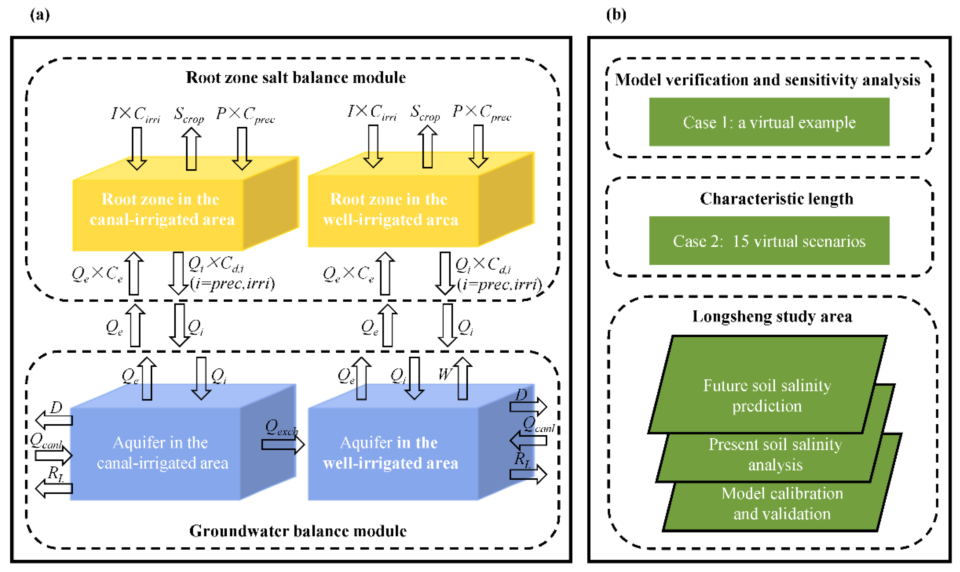
2.1. Model Development

The model was developed to quickly predict general trends in long-term soil salinization processes with simple obtained data, rather than for accurate predictions. Therefore, the model may be a helpful tool for pre-implementation planning analysis of well-canal conjunctive irrigation. The well-canal conjunctive irrigation concept described in the developed model is shown in Figure 1a, while a schematic presentation of the processes of the model verification and sensitivity analysis of the characteristic length, as well as the forecasting process of long-term soil salinity dynamics at the study site, are presented in Figure 1b. The groundwater balance module was firstly used to calculate the water fluxes’ processes in the canal-irrigated area and the well-irrigated area. Then the root zone salt balance module was used to access the salt dynamics in the root zone. In addition, the canal-irrigated and well-irrigated areas are linked by the lateral exchange flux through aquifers. The lateral water fluxes in the root zone are ignored since the horizontal gradient in the unsaturated zone is significant smaller than the vertical value in the unsaturated zone at the regional scale [23,39,42].

2.1.1. Groundwater Balance Module

• Groundwater balance in the well-canal conjunctive irrigation area

Eight items are considered in the developed groundwater balance model: seepage losses, percolation caused by irrigation and precipitation, exchange, drainage, lateral seepage, upward capillary rise from groundwater, and well pumping. The corresponding equations can be expressed as:

$$Q_{canl,j}+Q_{irri,j}+Q_{prec,j}+R_{L,j}+Q_{exch,j}-D_j-Q_{e,j}-W_j=\Delta Q_j,$$

(1)

$$Q_{canl,j}={\eta }_j\times J_j,$$

(2)

$$Q_{irri,j}={\alpha }_j\times I_j,$$

(3)

$$Q_{prec,j}={\lambda }_j\times P_j,$$

(4)

$$Q_{e,}{}_j={\epsilon }_j\times {\exp }^{-d_j\times h_j}\times E_{0,j},$$

(5)

$$\Delta Q_j=\Delta H_j\times {\mu }_j,$$

(6)

where the subscript j = canal or well denotes canal- or well-irrigated areas; Q_canl,j is the seepage losses from the canal system in the j-irrigated area (m); Q_irri,j and Q_prec,j are the downward percolation caused by irrigation and precipitation in the j-irrigated area, respectively (m); R_L,j is the lateral flux from external regions (m); Q_exch,j is the groundwater exchange in the j-irrigated area (m); D_j is the drainage in the j-irrigated area (m); Q_e,j is the upward capillary rise from groundwater in the j-irrigated area (m) and is assumed to depend on the water table depth and reference evapotranspiration, which was recommended by Wang [43] on the basis of experiments in the Hetao Irrigation District; W_j is the amount of water pumped in the j-irrigated area; J_j is the water in the canal system in the j-irrigated area (notably, this water is considered the diversion water and pumping water in the canal- and well-irrigated area, respectively); ΔQ_j is the storage change of groundwater in the j-irrigated area (m); η_j, α_j, and λ_j are the recharge coefficients of canal losses, irrigation, and precipitation in the j-irrigated area, respectively; I_j, P_j, and E_0,j are the irrigation, precipitation, and water surface evaporation values in the j-irrigated area, respectively (m); ε_j and d_j are the capillary rise coefficients in the j-irrigated area; h_j is the average water table depth in the j-irrigated area (m); and μ_j is the specific yield in the j-irrigated area. Notably, Q_exch,j is the key to implementing the coupling process.

2.

Water exchange between canal- and well-irrigated areas

The exchanged mass per unit area is described by Darcy’s law as follows:

$$Q_{exch,j}=KA\frac{H_{canal}-H_{well}}{L_c{A}_j}T,$$

(7)

where the subscript j = canal and well denotes the canal- and well-irrigated areas, respectively; K is the saturated hydraulic conductivity of the aquifer (m/d); A is the cross section of the well-canal conjunctive irrigated area and is available from the generalized boundary length and aquifer thickness (m²); A_j is the j-irrigated area (m²); H_j is the average groundwater level in the j-irrigated area (m); T is the calculation period (d); and L_c is the characteristic length of the well-canal conjunctive irrigation area (m). Since L_c cannot be measured directly, it is treated as a parameter in practical applications, and further discussion can be found in Section 2.2.1. Moreover, the parameter L_c is a synthetic parameter, which is related to the spatial topology of the layout of well-canal conjunctive irrigation, instead of a certain actual physical distance.

2.1.2. Root Zone Salt Balance Module

Six items are considered in the root zone salt balance module, including the salt inflows from irrigation, capillary rise, and precipitation and the salt outflows due to leaching through irrigation and precipitation and the uptake of salt by crops. The average salt salinity of the root zones in the canal- and well-irrigated areas can be calculated separately, and the equations are given as:

$$S_{irri,j}+S_{prec,j}+S_{e,j}-S_{d,}{}_{irri,j}-S_{d,}{}_{prec,j}-S_{crop,j}=\Delta S_j,$$

(8)

$$S_{irri,j}=I_j\times C_{irri}{}_{,j},$$

(9)

$$S_{prec,j}=P_j\times C_{prec,j},$$

(10)

$$S_{e,j}=Q_e{}_{,j}\times C_{e,j},$$

(11)

$$S_{d,}{}_{irri,j}=Q_{irri,j}\times C_{d,}{}_{irri,j},$$

(12)

$$S_{d,}{}_{prec,j}=Q_{prec,j}\times C_{d,}{}_{prec,j},$$

(13)

$$\Delta S_j=\Delta S{C}_j\times {\rho }_j\times h_{r,j}\times 100,$$

(14)

where the subscript j = canal and well denote the canal- and well-irrigated areas, respectively; S_irri,j, S_prec,j and S_e,j are the salt inputs to the root zone derived from irrigation, precipitation and capillary rise in the j-irrigated area, respectively (kg/m²); S_d,irri,j and S_d,prec,j are the amounts of salt leached from the root zone through irrigation and precipitation in the j-irrigated area, respectively (kg/m²); S_crop,j is the amount of salt taken up by crops in the j-irrigated area; ΔS_j is the storage change of salt in the root zone in the j-irrigated area (kg/m²); C_irri,j, C_prec,j and C_e,j are the concentrations of irrigation, precipitation and capillary rise water in the j-irrigated area, respectively (kg/m³); ΔSC_j is the change in the soil salt salinity of the root zone in the j-irrigated area (kg/100 kg); ρ_j is bulk density in the j-irrigated area (kg/m³); h_r,j is the depth of root zone in the j-irrigated area (m); C_d,irri,j and C_d,prec,j are the salt concentrations of the percolation at the bottom of the root zone in j-irrigated area due to irrigation and precipitation, respectively (kg/m³). C_d,irri,j and C_d,prec,j mainly depend on the salt concentrations of the soil solution and the irrigation or precipitation in the j-irrigated area, and can be calculated as follows:

$$C_{d,}{}_{i,j}=C_{i,j}\times (1-f_j)+C_{t,j}\times f_j(i=irri,prec),$$

(15)

$$C_{t,j}=S{C}_{a,j}\times {\rho }_j/{\theta }_{tc,j},$$

(16)

where C_t,j is the salt concentration of the soil solution in the j-irrigated area (kg/m³); f_j is the leaching efficiency in the j-irrigated area; SC_a,j is the salt salinity in the root zone of the j-irrigated area (kg/100 kg); and θ_tc,j is a water content used as a coefficient for transforming the soil salt salinity to the salt concentration. In this study, the coefficient is regarded as the average volumetric water content in the root zone within the simulation duration.

C_e,j is calculated under the assumption that it is proportional to the average salt concentration of the percolation at the bottom of the root zone using the following equation:

$$C_{e,j}={\beta }_j\times \frac{{\displaystyle \sum _{i=irri,prec}{C}_{d,i,j}\times Q_{i,j}}}{{\displaystyle \sum _{i=irri,prec}{Q}_i{}_{,j}}},$$

(17)

where β_j is the ratio of the salt concentration of the downward percolation to the salt concentration of the upward capillary rise at the bottom of the root zone in the j-irrigated area. This parameter is relatively stable under different soil textures and bottom boundary conditions and can be defined as a coefficient (Sun et al. [38]).

The water fluxes at the bottom of the root zone (Q_irri,j, Q_prec,j, and Q_e,j) are obtained by the groundwater balance module. Consequently, the root zone salt balance module needs only three parameters, i.e., f_j, θ_tc,j, and β_j, to calculate the root zone salt salinity in the j-irrigated area.

The relationship between the soil salinity and EC_e (the electric conductivity of an extract of a saturated soil paste, dS/m) can be obtained based on the regression equation [18,44], and is presented as, ${\mathrm{EC}}_{{e}}=27.52\times \mathrm{SS}-0.18$, where SS is the soil salinity (kg/100 kg).

2.2. Model Verification and Application

In this part, three cases are used to test the model. Case 1 is a synthetic virtual case in which the effect of the characteristic length L_c is investigated. Case 2 is used to demonstrate the value rule of the characteristic length L_c. Case 3 is a practical application in the Longsheng well-canal conjunctive irrigation district.

2.2.1. Case 1: Synthetic Virtual Case for the Model Verification and Sensitivity Analysis

1.

Model verification

In this case, the 3D groundwater flow under changing source and sink term conditions was designed, and the results calculated by MODFLOW were used as the reference values. The study site is 20,000 m long and 10,000 m wide; half of this region is canal-irrigated, and the other half is well-irrigated. The depth of the aquifer is 100 m, and the specific yield and horizontal hydraulic conductivity of the aquifer are 0.1 and 10 m/d, respectively. In MODFLOW, the canal- and well-irrigated areas are spatially dispersed into 100 grids with lengths of 100 m and widths of 100 m. Figure 2 shows the source and sink terms of the case study, including the local precipitation, irrigation, pumping water and water surface evaporation (E₀) conditions. The initial water table depths in the canal- and well-irrigated areas are 2.5 m and 3.5 m, respectively. The simulation duration is 2140 days; this duration is divided into 10 calculation cycles based on the irrigation and pumping water conditions. It is assumed that the first 153 days of each simulation cycle is the crop growth season and that the next 61 days is the no-crop period. The time step of MODFLOW is 1 day. Additionally, the irrigation schemes of the canal- and well-irrigated areas are the same, but the irrigation sources are different; during the crop-growing season, the canal- and well-irrigated areas use surface water and groundwater, respectively, while surface water is used in both areas during the no-crop period.

2.

Model sensitivity analysis

The characteristic length of the well-canal conjunctive irrigated area (L_c) cannot be calculated using the developed model and is treated as a parameter in practical applications. However, the parameter value has a certain impact on the simulation results; thus, performing a sensitivity analysis that identifies whether L_c significantly influences the model outputs is necessary. The L_c value obtained during the above model-validation step is taken as the default value. Then, the L_c default value is altered using ±70% perturbations to obtain varying simulation results from the WSBM. A widely used elasticity formula [35,45,46] was applied to determine the sensitivity of the water table depth to the characteristic length parameter L_c; this indicator was calculated as follows:

$$\Phi =\frac{\Delta O/O}{\Delta I/I},$$

(18)

where Φ is the elasticity; O and I are the model outputs and the input model parameters, respectively; ΔI/I is the change ratio of the input parameters; ΔO/O is the change ratio of the outputs when the input parameters change. Values of Φ > 0 indicate that the outputs and the input parameters change in the same direction and vice versa. The greater the |Φ| value is, the more sensitive the model outputs are to the input parameters. Generally, parameters with |Φ| values > 1 are categorized as sensitive parameters, while parameters with |Φ| values < 1 are categorized as less sensitive parameters.

2.2.2. Case 2: Synthetic Case for the Parameter Value Rule

The WSBM cannot consider the actual spatial location of the canal-irrigated area or the well-irrigated area because of the lumped model structure. However, the L_c value is deeply influenced by the real-world spatial distance between the canal- and well-irrigated areas. Therefore, two special real-world spatial location schemes are considered to illustrate the value rule. In the first scheme, the canal- and well-irrigated districts are adjacent (Figure 3a). In the second scheme, the canal- and well-irrigated areas have central symmetry (Figure 3b). For each of these location schemes, different canal- and well-irrigated area sizes are set, as listed in

Table 1. Different sizes of canal- and well-irrigated areas in two special spatial locations.

Spatial Locations	Scenario No.	Sizes of Canal-Irrigated Area (×104 m2)	Sizes of Well-Irrigated Area (×104 m2)	Center Distance (m)	Lc (m)
Adjacent	A1	70	30	500	333
	A2	50	50		333
	A3	30	70		333
	A4	140	60	1000	667
	A5	100	100		667
	A6	60	140		667
	A7	210	90	1500	1000
	A8	150	150		1000
	A9	90	210		1000
Central symmetry	A10	84	16	350	233
	A11	64	36	400	267
	A12	36	64	450	300
	A13	336	64	700	467
	A14	256	144	800	533
	A15	144	256	900	600

, where the sizes are marked as A1–A15. L_c is set as 2/3 of the distance between the centers of the canal-irrigated and well-irrigated areas [47], and the WSBM performance is evaluated using the MODFLOW results derived under the same conditions.

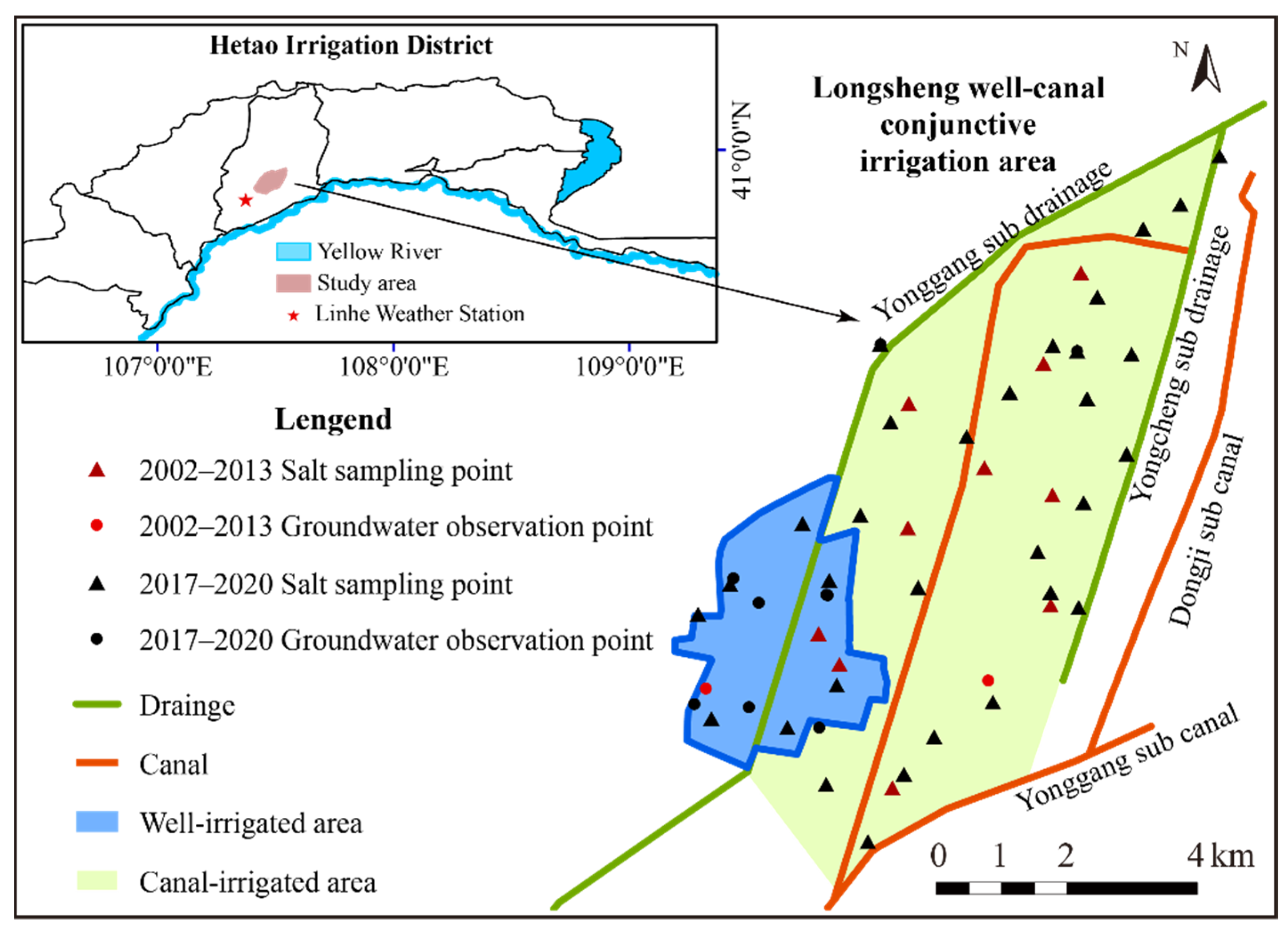
2.2.3. Case 3: Practical Application in an Arid Agricultural District

1.

Study site

The Longsheng irrigation district (107°28′ E–107°32′ E, 40°51′ N–107°32′ N) is located in the central region of the Hetao Irrigation District, Inner Mongolia, China, as shown in Figure 4. The canal-irrigated area is approximately 36.67 km² in size, while the well-irrigated area is 900 km² in size. The agricultural land utilization rates in the canal- and well-irrigated areas are 0.76 and 0.52, respectively. The spatial variability of soil properties in the horizontal direction in the study area is not very strong, while there is significant soil stratification in the vertical direction. The soil texture in the root zone of Longsheng irrigation district is mainly loam and sandy loam, with bulk density ranging from 1.45 g/cm³ to 1.55 g/cm³ and porosity ranging from 46.43% to 49.73%. Moreover, the study area is dominated by sandy soils below 1 m. [48]. The thickness of the aquifer is 100 m below the land surface [18].

Based on the measured climate and crop growth characteristics, the whole year is divided into three seasons. Season 1 is the crop growth period and lasts from May to September. Season 2 is the autumn irrigation period lasting from October to November. Crops are planted once a year from May to September in this study area, and the intensive irrigation in autumn, which consumes almost one-third of the total amount of diverted water in a year, was used to leach soil salt from the root zone after harvest. The freezing-thawing period lasts from December to April of the following year and is denoted as Season 3. Notably, the soil water mechanisms that occur during the freezing-thawing period are different from those that dominate during other periods. During the freezing-thawing period, the water table depth dynamics are not caused by irrigation, precipitation or evaporation but are caused by the freezing or thawing of soil water, thus resulting in a water table drop or rise. In this study, an empirical method developed by Tong et al. [49] was used to correlate the phreatic evaporation coefficient with the water table depth during the freezing-thawing period as follows:

$$Q_{e,s3}=({\epsilon }_{s3}\times {\exp }^{-d_{s3}\times h_{s3}}+c_{s3})\times E_{0,s3},$$

(19)

where the subscript s3 represents the freezing-thawing period and c_s3 is an additional constant term. The developed model supposes that the soil salt salinity in the root zone after the freezing-thawing period is equal to the values before the freezing-thawing period.

Meteorological data recorded from 2002 to 2013 were collected from the Linhe Weather Station, including monthly evaporation data measured using a 20-cm evaporation pan (E_pan) and precipitation data. The Linhe Weather Station, which is a national meteorology monitoring station of China with a long series of observations, exists 18 km southwest of the study area as shown in Figure 4, and uniform meteorological data was used for the study area. The water surface evaporation (E₀) was then estimated by multiplying E_pan with a coefficient of 0.56 [49]. Water diversion data in the canal-irrigated areas from 2002 to 2013 was provided by the local water management department, and the average salt concentration was 0.64 g/L. The water table depth data observed every 5 days from 2002 to 2013 were obtained from two conventional groundwater observation wells. The correlation analysis with another seven short-term observation wells from 2002 to 2005 proved that the data from these two long-term observation wells can represent the variation of regional-scale groundwater table depth. In addition, data were collected from 9 observation wells that recorded measurements once every 10 days from 2017 to 2020. For the soil salt salinity, 10 soil sampling points were measured 4 times every year before 2013. Among them, a continuous series were obtained for the 2002–2005 and 2009–2010 periods, while a single measurement was obtained for 2013. Moreover, 32 soil samples were measured twice per year from 2017 to 2020. All sampling points were manually drilled and sampled, and the soil salinity is measured using a 1:5 soil-to-water extraction method. In addition, each sampling point was sampled every 20 cm below ground surface, to a total depth of 1 m, which is equal to the thickness of the root zone used in the study.

The annual average data were used in the simulation. The total precipitation in Seasons 1, 2 and 3 were 129.1 mm, 11.5 mm and 8.2 mm, respectively. The total water surface evaporation in Seasons 1, 2 and 3 were 891.9 mm, 117.9 mm and 287.4 mm, respectively. The water diverted in the canal-irrigated area was 585 mm per unit area during the crop growth period. The irrigation water pumped by wells in the well-irrigated area was 563 mm per unit area during the crop growth period. The amount of autumn irrigation in both the canal- and well-irrigated farmland were 300 mm per unit area. The initial water table depths in the canal- and well-irrigated areas were 1.8 m and 2.3 m, respectively, representing the average observation values derived over the studied years. The initial salt concentration in the root zone was set as the average observations at the beginning of the year 2002. The salt concentration of the groundwater in the Longsheng irrigation area was 1.2 kg/m³. The water table depth and soil salinity data observed from 2002 to 2005 and from 2006 to 2020 were used to calibrate and validate the developed model, respectively.

2.

Settings of the water-saving irrigation scenario

The irrigation quota in the crop growth period and autumn irrigation period, water table depth, and groundwater salt concentration all affect the root zone salinity dynamics in the irrigated district. Hence, the factors mentioned above must be considered in the canal- and well-irrigated districts. In fact, due to the coupling between the canal- and well-irrigated areas, different irrigation schemes (including the irrigation quotas in season 1 and season 2) can both affect the canal- and well-irrigated areas. Therefore, 15 scenarios were set, marked as S1–S15, as listed in

Table 2. Water-saving irrigation scenarios in canal- and well-irrigated areas.

Items	Scenario No.	Canal-Irrigated Area	Well-Irrigated Area
A. Irrigation quota in season 1 (mm)	S1	526.5	506.3
	S2	585.0	562.5
	S3	643.5	618.8
B. Irrigation quota in season 2 (mm)	S4	300	300
	S5	240	240
	S6	180	180
	S7	120	120
C. Water table depth (m)	S8	1.4	1.95
	S9	1.7	2.25
	S10	2.0	2.55
	S11	2.3	2.85
	S12	2.6	3.15
D. Groundwater salinity (kg/m3)	S13	0.64	1.2
	S14		2.0
	S15		3.0

. The irrigation quotas in the crop growth period were set as 90%, 100%, and 110% of the present values, corresponding to values of 526.5 mm, 585.0 mm, and 643.5 mm, respectively, in the canal-irrigated area and 506.3 mm, 562.5 mm, 618.8 mm, respectively, in the well-irrigated area. Values corresponding to 100%, 80%, 60%, and 40% of the current autumn irrigation quotas were considered, namely, 300 mm, 240 mm, 180 mm, and 120 mm, respectively, in both the canal- and well-irrigated areas. As stated before, there is an interaction between the water table depths in the canal- and well-irrigated areas, and the corresponding current water table depths are 2.0 m and 2.55 m, respectively. Thus, water table depths of 1.4 m, 1.7 m, 2.0 m, 2.3 m, and 2.6 m were considered in the canal-irrigated area by increasing or decreasing by a certain amount of 0.3 m based on the current value, corresponding to water table depths of 1.95 m, 2.25 m, 2.55 m, 2.85 m, and 3.15 m, respectively, in the well-irrigated area. In addition, three different groundwater salt concentrations were set: 1.2 kg/m³, 2.0 kg/m³, and 3.0 kg/m³. The initial root zone salt salinity of the canal- and well-irrigated areas in all the simulation scenarios were set as 0.108 kg/100 kg and 0.107 kg/100 kg, respectively. The further change in climate data did not incorporate because the soil salt accumulation and leaching processes were more influenced by irrigation and drainage than by climate data in the arid agricultural regions, and the current average meteorological information was adopted.

2.3. Model Evaluation Indexes

The mean relative error (MRE), normalized root mean square error (NRMSE), determination coefficient (R²) and Nash–Sutcliffe model efficiency (NSE) were used as evaluation indicators to assess the model performance. These indicators can be defined as follows:

$$MRE=\frac{1}{n}\sum _{i=1}^n\frac{(P_i-O_i)}{O_i}\times 100\%$$

(20)

$$NRMSE=\frac{\sqrt{\frac{{\displaystyle \sum _{i=1}^n{(P_i-O_i)}^2}}{n}}}{\frac{1}{n}{\displaystyle \sum _{i=1}^n{O}_i}}\times 100\%,$$

(21)

$$R^2={\left[\frac{{\displaystyle \sum _{i=1}^n(O_i-\overline{O_i})(P_i-\overline{P_i})}}{{\left[{\displaystyle \sum _{i=1}^n{(O_i-\overline{O_i})}^2}\right]}^{0.5}{\left[{\displaystyle \sum _{i=1}^n{(P_i-\overline{P_i})}^2}\right]}^{0.5}}\right]}^2,$$

(22)

$$NSE=1-\frac{{\displaystyle \sum _{i=1}^n{(P_i-O_i)}^2}}{{\displaystyle \sum _{i=1}^n{(O_i-\overline{O_i})}^2}},$$

(23)

where n is the total number of results; P_i and $\overline{P_i}$ are the ith model-predicted result and its mean value, respectively; and O_i and $\overline{O_i}$ are the ith reference result and its mean value, respectively (i = 1, 2, …, n).

3. Results and Discussion

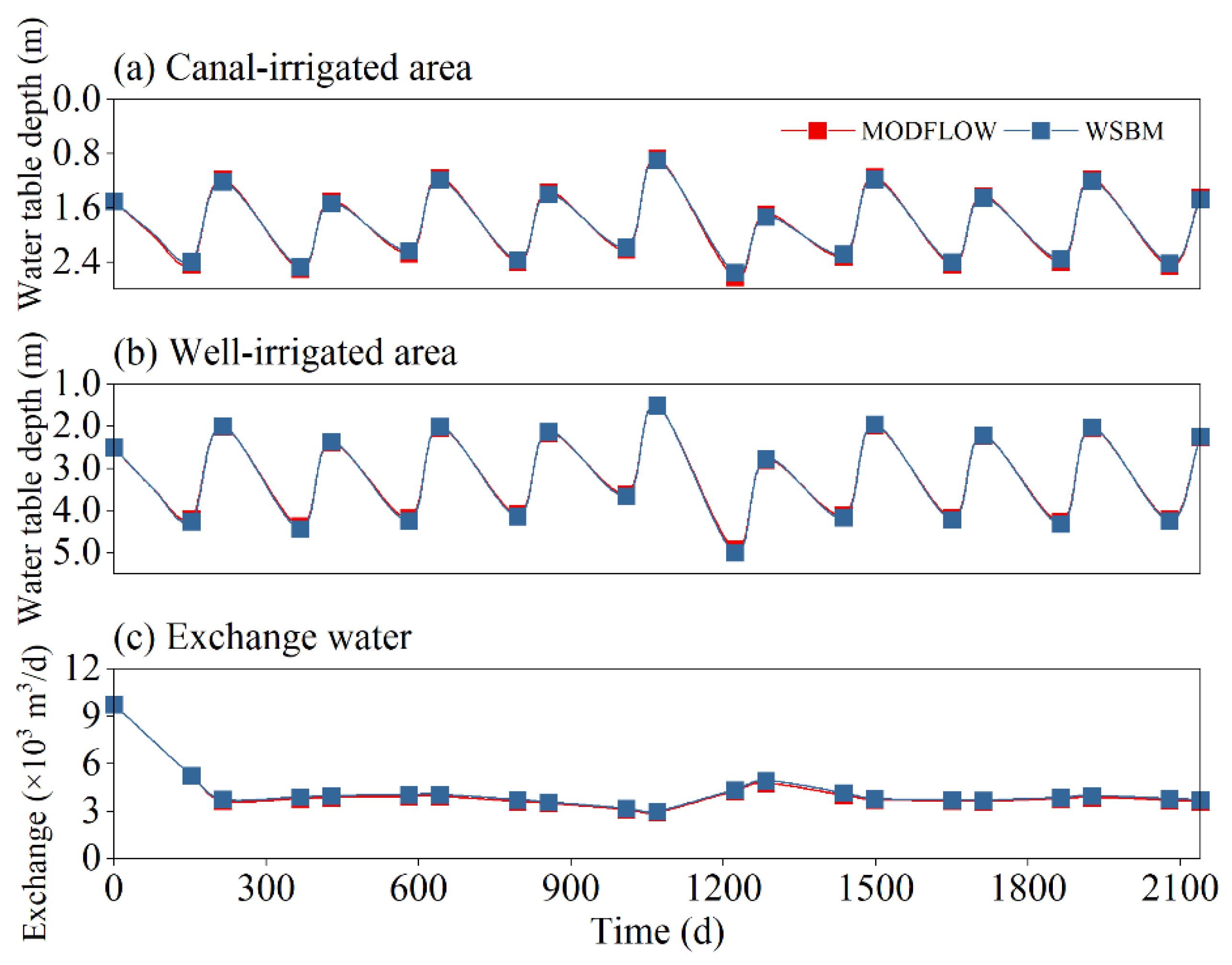
3.1. Model Accuracy of the Groundwater Balance Module

The percentage errors of mass balance calculated by MODFLOW are less than 0.03%, which indicates that it is reliable to choose MODFLOW results as the reference values. The virtual example with complicated boundary conditions (temporally varying precipitation, irrigation, pumping, and phreatic evaporation) considered under case 1 is used to test the groundwater balance module. The simulated water table depths in the canal- and well-irrigated areas derived from the developed model and MODFLOW are shown in Figure 5a,b. The MRE, NRMSE, R², and NSE values of the water table depth in the canal-irrigated area are 0.035%, 1.955%, 0.999, and 0.996, respectively; the corresponding values are 0.039%, 1.361%, 0.999, and 0.998, respectively, in the well-irrigated area, indicating that the WSBM can effectively obtain water table depth information in the canal- and well-irrigated areas. Moreover, the groundwater exchange simulated by the WSBM matches the value calculated by MODFLOW well, as shown in Figure 5c; the MRE, NRMSE, R², and NSE values are 2.393%, 2.363%, 0.999, and 0.995, respectively, showing that the water exchange between the canal- and well-irrigated areas can be well captured by the developed model. Based on the above results, the groundwater balance module is found to be credible.

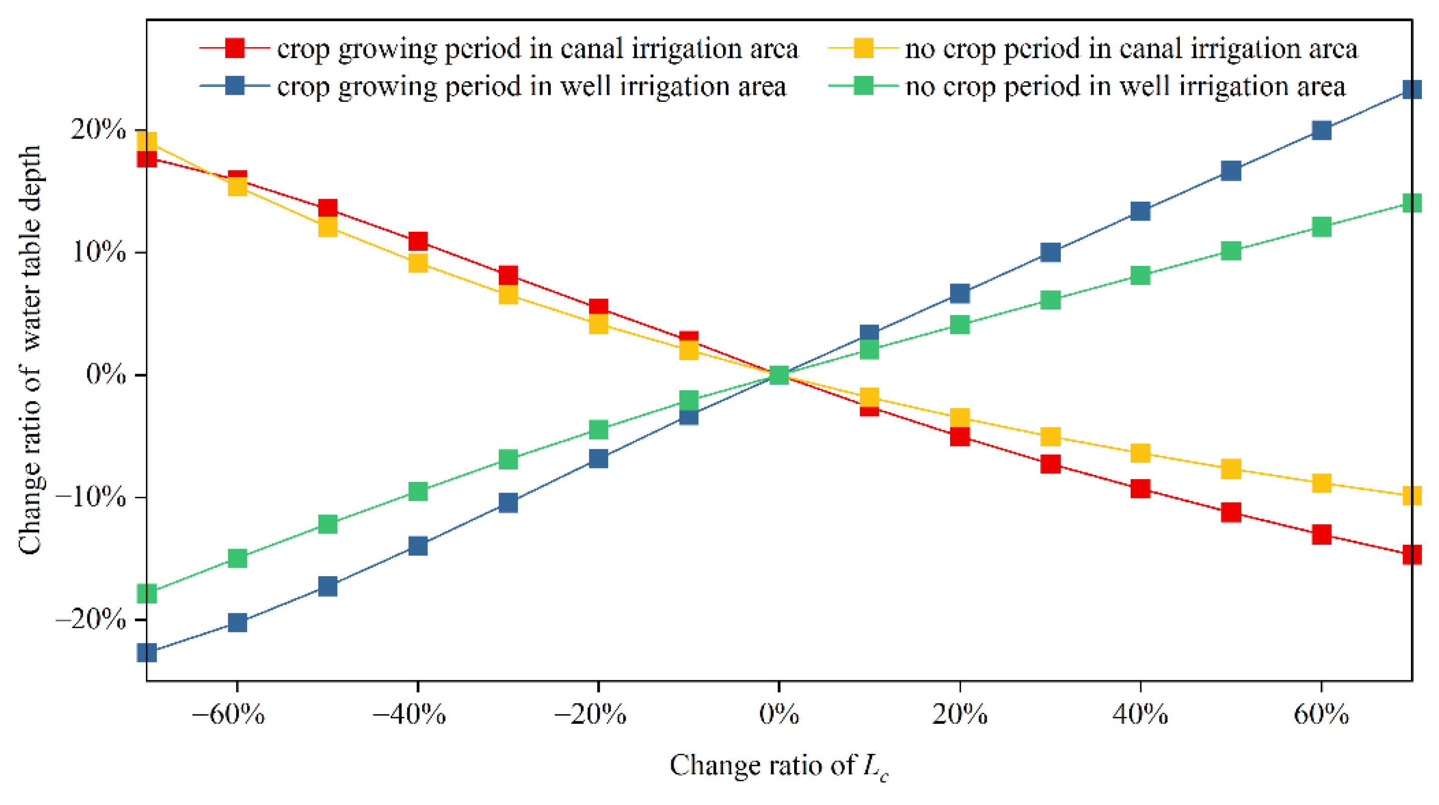
3.2. Model Sensitivity Analysis

Figure 6 shows the change ratio of the water table depth with the variation ratio of L_c. The elasticities of the water table depth in the canal- and well-irrigated areas are −0.278 and 0.349, respectively, during the crop growth period and −0.272 and 0.255, respectively, during the no-crop period. In detail, the L_c parameter has the greatest and least influence on the water table depth in the well-irrigated area during the crop growth and no-crop periods, respectively. Since the absolute values of all the elasticities are less than 1, L_c is categorized as an insensitive parameter. In other words, the sensitivity of the outputs to this input parameter is not significant.

3.3. Description of the L_c Parameter Value

Table 3. Model performance under 15 scenarios while L_c is two-thirds of center distance.

Scenario No.	Center Distance (m)	Lc (m)	Water Table Depth
			Canal-Irrigated Area				Well-Irrigated Area
			R2 (-)	NRMSE (%)	MRE (%)	NSE (-)	R2 (-)	NRMSE (%)	MRE (%)	NSE (-)
A1	500	333	1.000	0.569	0.006	1.000	1.000	0.486	0.006	1.000
A2		333	1.000	0.355	0.008	1.000	1.000	0.386	0.009	1.000
A3		333	1.000	1.923	0.083	0.995	1.000	1.799	0.080	0.995
A4	1000	667	1.000	0.794	0.008	1.000	1.000	1.947	0.030	0.999
A5		667	1.000	1.073	0.017	0.999	1.000	0.727	0.019	1.000
A6		667	0.998	2.459	0.097	0.991	1.000	1.265	0.055	0.998
A7	1500	1000	0.999	3.426	0.035	0.995	1.000	3.360	0.063	0.995
A8		1000	0.999	1.982	0.035	0.996	1.000	1.346	0.039	0.998
A9		1000	0.995	2.415	0.076	0.992	1.000	0.721	0.030	0.999
A10	350	233	0.999	4.111	0.032	0.996	0.999	4.387	0.041	0.996
A11	400	267	1.000	0.419	0.006	1.000	1.000	1.082	0.015	0.999
A12	450	300	0.999	2.191	0.071	0.994	0.999	2.433	0.083	0.991
A13	700	467	0.999	4.081	0.030	0.996	0.999	3.641	0.033	0.997
A14	800	533	1.000	0.964	0.013	1.000	1.000	2.657	0.036	0.997
A15	900	600	0.998	1.879	0.056	0.995	0.999	2.772	0.097	0.989

shows a comparison of the water table depths obtained by the WSBM and those obtained by MODFLOW under 15 scenarios in case 2. It can be found that the simulations of the WSBM are in high agreement with those of MODFLOW under A1–A15, thus indicating that the value law of L_c is reliable when the canal- and well-irrigated districts are adjacent (Figure 3a, A1–A9) or when the canal- and well-irrigated areas are centrally symmetric (Figure 3b, A10–A15). Although the WSBM can always find an appropriate L_c value to obtain reasonable simulations under the regular adjacent layout or central layout, it is recommended that this parameter be calibrated for real-world applications due to the complicated spatial layouts of canal- and well-irrigated areas in the real world.

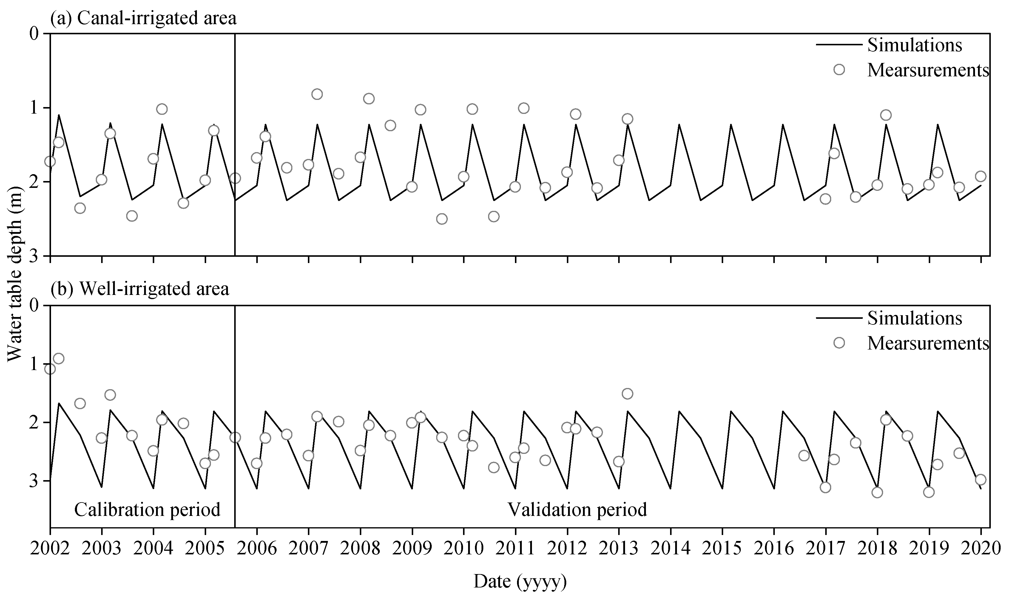
3.4. Model Calibration and Validation in the Longsheng Well-Canal Conjunctive Irrigation District

3.4.1. Model Calibration

The water table depths and soil salinity observed from 2002 to 2005 were used to calibrate the developed model. The comparison of the simulated water table depths and salt salinity of the root zone with the measured values during the calibration period are shown in Figure 7 and Figure 8. The simulated and measured water table depths and soil salinity of the root zone in the well-irrigated and canal-irrigated areas during the calibration period are listed in

Table 4. Model calibration results obtained by comparing the simulated and measured water table depths and root zone soil salinities.

Item	Season	Canal-Irrigated Area						Well-Irrigated Area
		Observation (m)	Simulation (m)	MRE (%)	NRMSE (%)	R2 (-)	NSE (-)	Observation (m)	Simulation (m)	MRE (%)	NRMSE (%)	R2 (-)	NSE (-)
Water table depth (m)	Season 1	1.84	2.00	8.74	8.70	0.20	−0.24	2.14	3.09	44.38	44.39	0.99	−0.11
	Season 2	1.29	1.19	7.87	15.50	0.47	0.19	1.74	1.77	1.74	27.59	0.75	0.65
	Season 3	2.37	2.23	5.91	7.59	0.61	0.88	2.05	2.26	10.20	10.24	0.79	0.45
	Annual	1.97	1.96	7.43	9.14	0.79	0.42	2.03	2.52	23.03	27.59	0.87	0.32
ECe (dS/m)	Season 1	5.43	5.38	1.13	15.20	0.21	0.40	5.35	4.77	10.31	24.38	0.22	0.19
	Season 2	4.75	4.31	8.88	8.94	0.95	−0.32	4.80	3.73	21.68	23.74	0.64	−1.28
	Season 3	5.93	4.53	23.14	22.97	0.95	0.63	4.17	3.92	5.96	13.29	0.97	0.44
	Annual	5.52	4.83	11.59	17.87	0.65	0.46	4.77	4.25	10.39	20.00	0.60	0.36

Note: the annual values in the table are a weighted average according to the length of the season.

. The MRE values of the annual water table depth in the canal- and well-irrigated areas are 7.43% and 23.03%, respectively, the NRMSE values are 9.14% and 27.59%, respectively, and the R² values are 0.79 and 0.87, respectively, and the NSE values are 0.42 and 0.32, respectively. The largest deviation occurs in season 1 in the well-irrigated area. This is because a large amount of groundwater is pumped for irrigation in the well-irrigated district during the crop growth period, leading to a significant variation in the water table depth calculated by the developed model. The above results indicate that the groundwater balance module is able to reasonably capture groundwater dynamics in canal- and well-irrigated areas. The calibrated parameters involved in the groundwater balance module are listed in

Table 5. Parameters of the developed model in the Longsheng well-canal conjunctive irrigation area.

A. Groundwater balance
μ (-)	η (-)	λ (-)	Season 1			Season 2			Season 3				Lc (m)	K (m/d)
			αs1 (-)	εs1 (-)	ds1 (-)	αs2 (-)	εs2 (-)	ds2 (-)	αs3 (-)	εs3 (-)	ds3 (-)	cs3 (-)
0.10	0.17	0.12	0.15	0.6601	0.898	0.40	0.6601	0.898	0	2	1	0	1200	10
B. Root zone salt balance
f (-)				θtc (cm3/cm3)					β (-)
0.80				0.28					0.99

Note: α_i, ε_i, d_i (i = s1, s2, s3) represent the coefficients in the crop growing period, autumn irrigation period, and freezing-thawing period respectively; all parameter values are identical both in the canal- and well-irrigated areas.

.

We further used the observed soil salinity of the root zone to calibrate the three parameters in the root zone salt balance module, i.e., f, θ_tc and β. The salt uptake by crops was set as 0.0225 kg/m² considering the widespread existence of salt-tolerant plants [49]. It can be seen from Table 4 and Figure 8 that in the three seasons, the largest MREs of the root zone soil salinity in the canal- and well-irrigated areas are 23.14% and 21.68%, respectively, corresponding to the largest NRMSE values of 22.97% and 23.74%, respectively. However, the MREs of the annual root zone soil salinity in the canal- and well-irrigated areas are 11.59% and 10.39%, respectively, the NRMSE values are 17.87% and 20.00%, respectively, the R² values are 0.65 and 0.60, respectively, and the NSE values are 0.46 and 0.36, respectively, indicating that the developed model can reasonably capture the average soil salinity of the root zone. The calibrated parameters used in the root zone salt balance module are listed in

Table 6. Model validation results by comparing the simulated and measured water table depths and root zone soil salinities.

Item	Season	Canal-Irrigated Area						Well-Irrigated Area
		Observation (m)	Simulation (m)	MRE (%)	NRMSE (%)	R2 (-)	NSE (-)	Observation (m)	Simulation (m)	MRE (%)	NRMSE (%)	R2 (-)	NSE (-)
Water table depth (m)	Season 1	1.92	2.05	6.78	8.85	0.45	0.54	2.62	3.13	19.45	20.23	0.33	0.32
	Season 2	1.18	1.22	3.69	22.03	0.22	0.13	2.17	1.81	16.64	19.35	0.42	0.59
	Season 3	2.13	2.25	5.73	14.08	0.43	0.67	2.36	2.27	3.78	8.05	0.56	0.47
	Annual	1.88	1.99	5.83	12.77	0.65	0.44	2.44	2.55	12.45	15.16	0.47	0.56
ECe (dS/m)	Season 1	3.26	3.32	2.06	11.20	0.36	0.25	3.48	3.34	3.45	12.78	0.38	0.29
	Season 2	2.96	2.79	5.38	20.18	0.26	0.02	3.51	2.68	22.89	30.60	0.27	0.15
	Season 3	2.60	2.65	1.23	7.92	0.62	0.24	3.04	2.63	12.57	17.09	0.64	0.46
	Annual	2.93	2.96	2.27	11.50	0.68	0.21	3.29	2.93	10.49	17.46	0.52	0.33

Note: the annual values in the table are a weighted average according to the length of the season.

. The f, θ_tc, and β values in the canal- and well-irrigated areas are the same. The f value used in the model is 0.80; this value is in accordance with the calibrated values obtained by [18,50]. The utilized θ_tc value is 0.28, which agrees with the field capacity of 0.25–0.3 determined in this area [49]. The β value is 0.99; this value was also obtained by Sun et al. [38] in the same study area. θ_tc is a soil water content used as a coefficient for transforming the soil salt salinity to the soil salt concentration and f is the leaching efficiency of the root zone, and both coefficients are mainly influenced by soil texture and are stable values for the specific study area from a long-term perspective. β is the ratio of the salt concentration of the downward percolation to the salt concentration of the upward capillary rise at the bottom of the root zone, which may stabilize around 1.0 as it was used to describe the long-term soil water and salt exchange between the root zone and the lower region of the root zone.

3.4.2. Model Validation

The calibrated parameters are used to simulate the water table depth and root zone soil salinity from 2006 to 2020 in the model validation process. The simulated and observed water table depths and root zone salt salinity from 2006 to 2020 are shown in Figure 7 and Figure 8, and the simulated and measured average water table depth and root zone soil salinity data recorded during the validation period and used in the validation analyses are listed in Table 6. The MRE values of the annual water table depth in the canal- and well-irrigated areas are 5.83% and 12.45%, respectively, the NRMSE values are 12.77% and 15.16%, respectively, and the R² values are 0.65 and 0.47, respectively, and the NSE values are 0.44 and 0.56, respectively. The results listed above indicate good agreement between the simulated and measured water table depths. The MREs of the annual root zone soil salinity in the canal- and well-irrigated areas are 2.27% and 10.49%, respectively, the NRMSE values are 11.50% and 17.46%, respectively, the R² values are 0.68 and 0.52, respectively, and the NSE values are 0.21 and 0.33, respectively. The performance in season 2 is slightly worse than those in the other seasons, as the significant spatial variations seen in the soil salinity and root zone soil salinity data obtained by the WSBM dropped significantly after the autumn irrigation period. Generally, the aforementioned results are acceptable considering the difficulty in predicting soil salinity due to its strong spatiotemporal variability.

In summary, the developed model performs well for calculating the water table depths and root zone soil salinities in both canal- and well-irrigated areas.

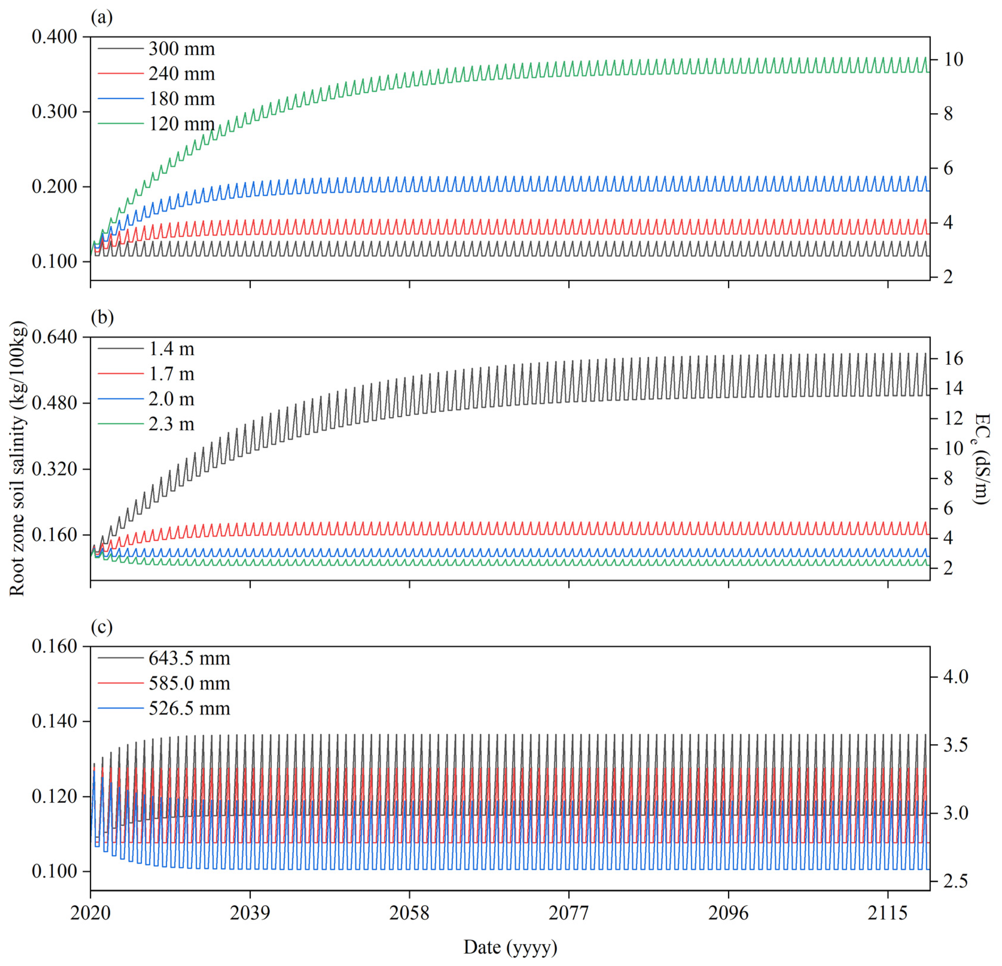
3.5. Long-Term Predictions of Soil Salinity Dynamics under Present and Future Water-Saving Conditions

The calibrated and validated model described above is used as a tool to predict the soil salinity dynamics over the next 100 years under current and future water-saving conditions, thus providing useful references for the sustainable development of agriculture.

3.5.1. Prediction Results under Present Conditions

Soil is considered non-saline when its salt salinity is less than 0.2 kg/100 kg (EC_e 5.32 dS/m); thus, a value of 0.2 kg/100 kg is applied here as the threshold. The predicted root zone soil salinity dynamics under current conditions are shown in Figure 9. The root zone soil salinity achieves a steady state and is far less than 0.2 kg/100 kg in both the canal- and well-irrigated areas under the current irrigation schemes, as shown in Figure 9; this result indicates that the current conditions meet the requirements of crop growth.

A mass equilibrium analysis is carried out to identify the major factors affecting the water and salt balance and to verify the rationality of the predictions, and the results are presented in

Table 7. Annual average mass balance under current conditions.

Water Balance Items		Canal-Irrigated Area		Well-Irrigated Area
		mm	Proportion (%)	mm	Proportion (%)
Iteams of inflow	Percolation from irrigation in season 1	55.35	21.03	36.45	8.56
	Percolation from irrigation in season 2	75.7	28.76	51.79	12.16
	Seepage from canal system in season 1	75.58	28.71	49.77	11.68
	Seepage from canal system in season 2	38.76	14.72	26.52	6.23
	Percolation from precipitation	17.86	6.78	17.86	4.19
	Recharged exchange water	0	0.00	243.61	57.19
	Total recharge	263.25	100.00	426.00	100.00
Iteams of outflow	Phreatic evaporation in season 1 and season 2	107.85	40.97	54.66	12.83
	Groundwater moving upward to the frozen layer in season 3	95.61	36.32	78.57	18.44
	Discharged exchange water	59.79	22.71	0.00	0.00
	Pumping water	0	0.00	292.76	68.72
	Total discharge	263.25	100.00	425.99	100.00
Salt Balance Items		Canal-Irrigated Area		Well-Irrigated Area
		kg/m2	Proportion (%)	kg/m2	Proportion (%)
Iteams of inflow	Salt from irrigation in season 1	0.311	31.90	0.561	57.39
	Salt from irrigation in season 1	0.159	16.36	0.159	16.31
	Salt from phreatic evaporation in season 1	0.405	41.60	0.206	21.09
	Salt from phreatic evaporation in season 2	0.099	10.14	0.051	5.20
	Total inflow	0.974	100.00	0.977	100.00
Iteams of outflow	Salt leaching by irrigation in season 1	0.335	34.38	0.326	33.41
	Salt leaching by irrigation in season 2	0.541	55.45	0.552	56.51
	Salt leaching by precipitation	0.077	7.86	0.076	7.77
	Salt uptake by crop	0.023	2.31	0.023	2.30
	Total outflow	0.975	100.00	0.977	100.00

. In the canal-irrigated area, percolation from irrigation and phreatic evaporation are the major processes affecting groundwater recharge and discharge, respectively; in the well-irrigated area, these processes are water exchange and pumping, respectively (Table 7a). In the canal-irrigated area, the salt source is mainly phreatic evaporation, with a quantity of 0.504 kg/m² per year, constituting 51.74% of all input salt. Leaching from autumn irrigation is the main factor affecting salt discharge in the canal-irrigated area, contributing 0.541 kg/m² per year and accounting for 55.45% of the total output salt. In the well-irrigated area, irrigation water derived from groundwater is the main source of input salt, inputting an amount of 0.561 kg/m² per year or 57.39% of the total input salt. The salt discharge in the well-irrigated area is principally contributed to leaching from autumn irrigation, which contributes 0.552 kg/m² of salt per year, accounting for 56.51% of the total output salt. In both the canal- and well-irrigated areas, the salt input is equal to the salt output under current conditions; no salt accumulation occurs in the root zone, and this is consistent with the derived prediction results.

3.5.2. Prediction Results Obtained under Future Water-Saving Conditions

The soil salinity dynamics in the root zone under different autumn irrigation schemes in the canal- and well-irrigated areas are shown in Figure 10a and Figure 11a, respectively. There are obvious increases in the soil salt salinity in the canal- and well-irrigated areas as the autumn irrigation decreased. The predicted soil salt salinity at the end of the crop-growing period after 100 years are approximately 0.214 kg/100 kg (EC_e 5.71 dS/m) and 0.204 kg/100 kg (EC_e 5.43 dS/m) in the canal- and well-irrigated areas, respectively, corresponding to 60% and 40% of the current autumn irrigation level, respectively; both areas are thus categorized as mildly saline lands according to the relevant classification criteria and can meet the growth requirements of most crops. Therefore, autumn irrigation quotas of 180 mm in the canal-irrigated area and 120 mm in the well-irrigated area are recommended if the goal is only to maintain the lack of salt accumulation in the root zone.

Figure 10b and Figure 11b show the soil salinity dynamics in the canal- and well-irrigated areas at different water table depths. The soil salt salinity is obviously affected by the water table depth in the canal-irrigated area with a shallow water table depth but is slightly affected in the well-irrigated area, which has a deeper water table depth. The reason for this phenomenon is that the relationship between phreatic evaporation and the water table depth is nearly a negative exponential correlation. Therefore, when the same variation in water table depth occurs, the changes in capillary rising water are larger in shallow groundwater areas than in deep groundwater areas, leading to more salt being input into the root zone. As a result, increasing the water table depth to reduce capillary rise is an effective way to control soil salinization in canal-irrigated areas. However, due to the less obvious changes in soil salinity that occur in the root layer when the groundwater levels in deep water table depth areas are increased, increasing the water table depth to control soil salinization in well-irrigated areas is not recommended. In addition, the root zone soil salinity in the canal-irrigated area is close to 0.2 g/kg when the water table depth is 1.7 m (Figure 10b); thus, it is suggested that the water table depth in this region can be controlled below 1.7 m under the current conditions. When the water table depth in the well-irrigated area is 1.95 m, the soil salinity of the root zone is slightly more than 0.2 g/kg (Figure 11b); thus, the water table depth should not decrease below 1.95 m under the current conditions.

The root zone soil salinity dynamics observed under different irrigation quotas during the crop-growing period in the canal- and well-irrigated areas are shown in Figure 10c and Figure 11c, respectively. It can be seen that the irrigation water in the crop-growing period has little effect on the soil salt salinity in the canal- and well-irrigated areas, yet the salt salinity in the root zone is relatively high when more irrigation water is used and vice versa. This is because the salt input from irrigation is greater than the salt leaching, and most salt in irrigation water remains in the root zone. In general, different irrigation quotas play a slight role influencing the variation in the root zone salt salinity.

Figure 11d shows the soil salinity dynamics in the well-irrigated area under different groundwater salt concentrations. The root zone salt salinity and its amplitude throughout the different periods in a year visibly increase with the groundwater salinity. This may result from the fact that when the irrigation schemes remain unchanged, the higher the groundwater salinity is, the more salt is inputted and thus the more salt is leached, leading to violent variations in the soil salinity throughout the year. According to the prediction results shown in Figure 11d, when the groundwater salinity is 2.0 kg/m³, the soil salt salinity 100 years in the future is predicted to be 0.204 kg/100 kg (EC_e 5.43 dS/m), which is slightly more than 0.2 kg/100 kg (EC_e 5.32 dS/m) and far less than 0.3 kg/100 kg (EC_e 8.08 dS/m), thus basically meeting the crop growth demand. However, the soil salt salinity is 0.294 kg/100 kg (EC_e 7.91 dS/m) when the groundwater salinity is 3.0 kg/m³; this result is very close to the crop salt tolerance threshold. Consequently, the use of groundwater with mineralization concentrations less than 2.0 kg/m³ is advised for irrigation in well-irrigated areas from the perspective of sustainable agricultural development.

Given that autumn irrigation is a key factor in controlling the soil salinity in the root zone, which is used to leach soil salt out of the root zone after harvest. Figure 12 shows the required amounts of autumn irrigation water calculated by the model to sustain the root zone within the mild salinity level (0.3 kg/100 kg) under different water table depths in the canal-irrigated area, while Figure 13 shows the required amounts of autumn irrigation water under different groundwater salinities and water table depths in the well-irrigated area. These results indicate that (1) logarithmic relationships can be seen between the required autumn irrigation water amounts and water table depths in both the canal- and well-irrigated areas, and less autumn irrigation water is needed when the water table depth is deeper (Figure 12a and Figure 13a); (2) a linear relationship is observed between the required autumn irrigation water amount and groundwater salinity in the well-irrigated area, and higher groundwater salinity concentrations require more autumn irrigation water (Figure 13b); (3) the required autumn irrigation water amount can be decreased by 17.5 mm with an increase of 0.1 m in the water table depth in the canal-irrigated area under current conditions; and (4) the required amount of autumn irrigation can decrease by 22.2 mm with a 0.1 m increase in the water table depth and can increase by 101.7 mm with a 1.0 kg/m³ increase in the groundwater salinity.

4. Conclusions

A water and salt balance model (WSBM) for well-canal conjunctive irrigation was developed in this study by coupling canal- and well-irrigated areas using Darcy’s law. Three cases are designed to evaluate the performance of the WSBM by comparing the results with those obtained by the MODFLOW model and with measurements. A further discussion regarding the model parameter L_c is also included. Long-term soil salt predictions in the Longsheng well-canal irrigated areas in the Hetao Irrigation District are presented. The major conclusions are as follows:

(1)

The developed model can reasonably reflect the dynamics of groundwater and soil salinity in the root zone under well-canal conjunctive irrigation conditions, and the special parameter L_c in the model is not insensitive.

(2)

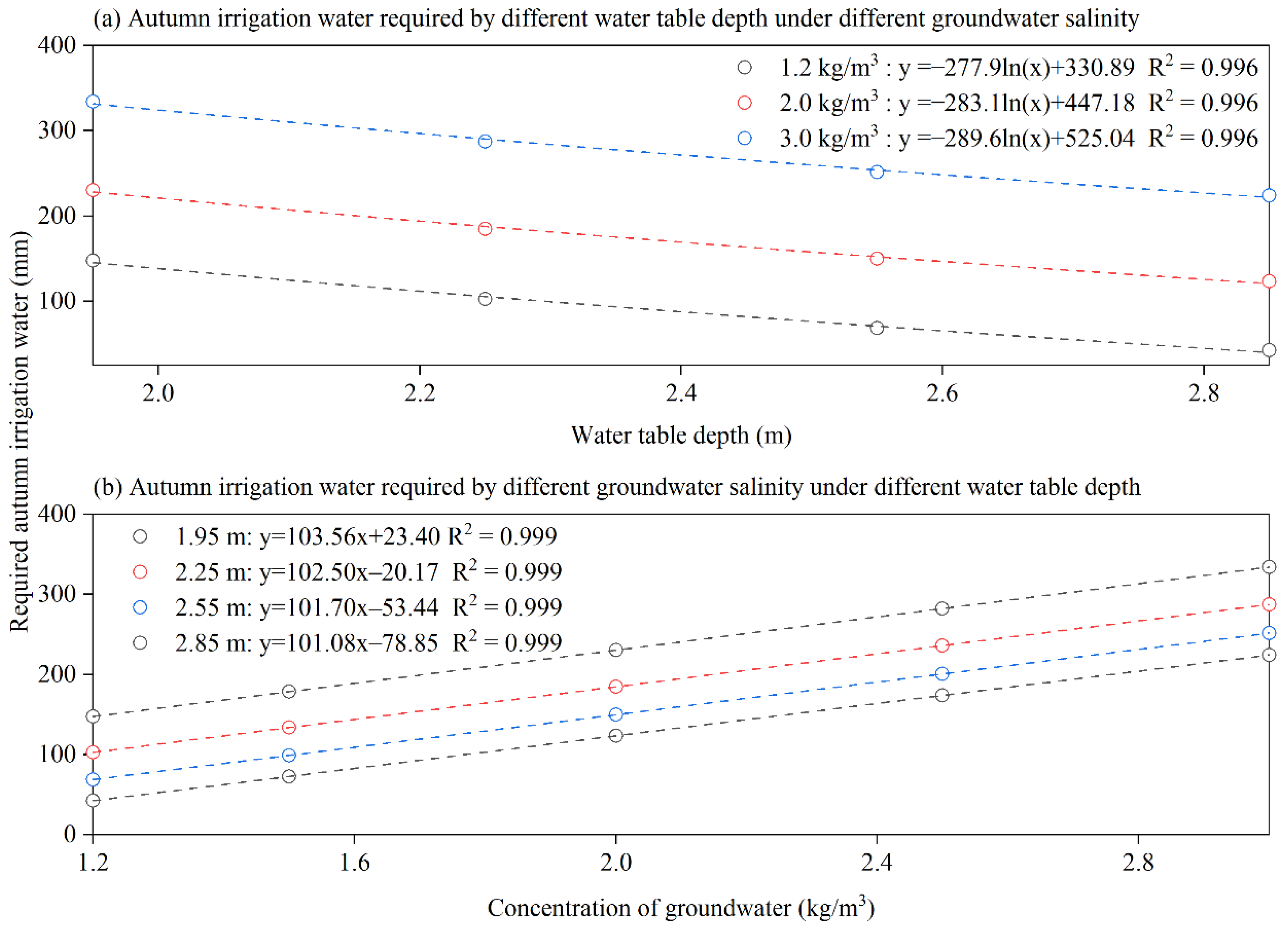
The soil salinity of the study area can be maintained at a low level under current conditions. Besides for water-saving conditions, the autumn irrigation amount for canal- and well-irrigated areas can decrease by 17.5 mm and 22.2 mm, respectively, with a 0.1 m increase in water table depth to maintain the soil salinity at a mild level, while an increase by 101.7 mm with a 1.0 kg/m³ groundwater concentration increase can occur in the well-irrigated area.

(3)

To effectively control soil salinization, the water table depth should be controlled at a suitable depth. For the canal-irrigated area, sufficient water for soil salt leaching should be guaranteed, while for the well-irrigated area, it is recommended to exploit groundwater with lower salt concentration.

(4)

The model is limited to regional-scale and large time discretization soil salinity prediction.

References

1. Kulmatov, R.; Khasanov, S.; Odilov, S.; Li, F. Assessment of the Space-Time Dynamics of Soil Salinity in Irrigated Areas under Climate Change: A Case Study in Sirdarya Province, Uzbekistan. Water Air Soil Pollut. 2021, 232, 216. [Google Scholar] [CrossRef]
2. Rengasamy, P. World salinization with emphasis on Australia. J. Exp. Bot. 2006, 57, 1017–1023. [Google Scholar] [CrossRef] [PubMed] [Green Version]
3. Fei, W.; Zhou, S.; Asim, B.; Shengtian, Y.; Jianli, D. Multi-algorithm comparison for predicting soil salinity. Geoderma 2019, 365, 114211. [Google Scholar]
4. Hassani, A.; Azapagic, A.; Shokri, N. Predicting long-term dynamics of soil salinity and sodicity on a global scale. Proc. Natl. Acad. Sci. USA 2020, 117, 33017–33027. [Google Scholar] [CrossRef] [PubMed]
5. Ali, R.; Elliott, R.L.; Ayars, J.E.; Stevens, E.W. Soil Salinity Modeling over Shallow Water Tables. I: Validation of LEACHC. J. Irrig. Drain. Eng. 2000, 126, 223–233. [Google Scholar] [CrossRef]
6. Ali, R.; Elliott, R.L.; Ayars, J.E.; Stevens, E.W. Soil Salinity Modeling over Shallow Water Tables. II: Application of LEACHC. J. Irrig. Drain. Eng. 2000, 126, 234–242. [Google Scholar] [CrossRef]
7. Yu, R.; Liu, T.; Xu, Y.; Zhu, C.; Zhang, Q.; Qu, Z.; Liu, X.; Li, C. Analysis of salinization dynamics by remote sensing in Hetao Irrigation District of North China. Agric. Water Manag. 2010, 97, 1952–1960. [Google Scholar] [CrossRef]
8. Xu, X.; Huang, G.; Qu, Z.; Pereira, L.S. Assessing the groundwater dynamics and impacts of water saving in the Hetao Irrigation District, Yellow River basin. Agric. Water Manag. 2010, 98, 301–313. [Google Scholar] [CrossRef]
9. Ren, D.; Xu, X.; Hao, Y.; Huang, G. Modeling and assessing field irrigation water use in a canal system of Hetao, upper Yellow River basin: Application to maize, sunflower and watermelon. J. Hydrol. 2016, 532, 122–139. [Google Scholar] [CrossRef]
10. Loescher, W.; Chan, Z.; Grumet, R. Options for Developing Salt-tolerant Crops. HortScience 2011, 46, 1085–1092. [Google Scholar] [CrossRef] [Green Version]
11. Cheng, Y.; Lee, C.-H.; Tan, Y.-C.; Yeh, H.-F. An optimal water allocation for an irrigation district in Pingtung County, Taiwan. Irrig. Drain. 2009, 58, 287–306. [Google Scholar] [CrossRef]
12. Bredehoeft, J.D.; Young, R.A. Conjunctive use of groundwater and surface water for irrigated agriculture: Risk aversion. Water Resour. Res. 1983, 19, 1111–1121. [Google Scholar] [CrossRef]
13. Li, P.; Qian, H.; Wu, J. Conjunctive use of groundwater and surface water to reduce soil salinization in the Yinchuan Plain, North-West China. Int. J. Water Resour. Dev. 2018, 34, 337–353. [Google Scholar] [CrossRef]
14. Chang, L.-C.; Ho, C.-C.; Yeh, M.-S.; Yang, C.-C. An Integrating Approach for Conjunctive-Use Planning of Surface and Subsurface Water System. Water Resour. Manag. 2011, 25, 59–78. [Google Scholar] [CrossRef]
15. Mani, A.; Tsai, F.T.-C.; Kao, S.-C.; Naz, B.; Ashfaq, M.; Rastogi, D. Conjunctive management of surface and groundwater resources under projected future climate change scenarios. J. Hydrol. 2016, 540, 397–411. [Google Scholar] [CrossRef] [Green Version]
16. Singh, A. Conjunctive use of water resources for sustainable irrigated agriculture. J. Hydrol. 2014, 519, 1688–1697. [Google Scholar] [CrossRef]
17. Gleeson, T.; VanderSteen, J.; Sophocleous, M.A.; Taniguchi, M.; Alley, W.M.; Allen, D.; Zhou, Y. Groundwater sustainability strategies. Nat. Geosci. 2010, 3, 378–379. [Google Scholar] [CrossRef]
18. Mao, W.; Yang, J.; Zhu, Y.; Ye, M.; Wu, J. Loosely coupled SaltMod for simulating groundwater and salt dynamics under well-canal conjunctive irrigation in semi-arid areas. Agric. Water Manag. 2017, 192, 209–220. [Google Scholar] [CrossRef]
19. Yang, Y.; Yan, Z.; Wei, M.; Heng, D.; Ming, Y.; Jingwei, W.; Jinzhong, Y. Study on the Exploitation Scheme of Groundwater under Well-Canal Conjunctive Irrigation in Seasonally Freezing-Thawing Agricultural Areas. Water 2021, 13, 1384. [Google Scholar] [CrossRef]
20. Yue, W.; Gao, H.; Chen, A. Study on conjunctive use of water resources in Hetao Irrigation District of Inner Mongolia based on GAMS simulation and optimization. South-to-North Water Transf. Water Sci. Technol. 2013, 11, 12–16. (In Chinese) [Google Scholar]
21. Mao, W.; Yang, J.; Zhu, Y.; Ye, M.; Liu, Z.; Wu, J. An efficient soil water balance model based on hybrid numerical and statistical methods. J. Hydrol. 2018, 559, 721–735. [Google Scholar] [CrossRef]
22. Karandish, F.; Šimůnek, J. A comparison of the HYDRUS (2D/3D) and SALTMED models to investigate the influence of various water-saving irrigation strategies on the maize water footprint. Agric. Water Manag. 2019, 213, 809–820. [Google Scholar] [CrossRef] [Green Version]
23. Lyu, S.; Chen, W.; Wen, X.; Chang, A.C. Integration of HYDRUS-1D and MODFLOW for evaluating the dynamics of salts and nitrogen in groundwater under long-term reclaimed water irrigation. Irrig. Sci. 2019, 37, 35–47. [Google Scholar] [CrossRef]
24. Hanson, B.; Hopmans, J.W.; Šimůnek, J. Leaching with Subsurface Drip Irrigation under Saline, Shallow Groundwater Conditions. Vadose Zone J. 2008, 7, 810–818. [Google Scholar] [CrossRef] [Green Version]
25. Birgani, S.; Mohammadi, A.S.; Nasab, S.B. Evaluation of the SWAP model for simulation of soil salinity under condition using of saline irrigation water and maize cultivation. N. Y. Sci. J. 2015, 8, 19–24. [Google Scholar]
26. Singh, R. Simulations on direct and cyclic use of saline waters for sustaining cotton–wheat in a semi-arid area of north-west India. Agric. Water Manag. 2004, 66, 153–162. [Google Scholar] [CrossRef]
27. Kroes, J.G.; van Dam, J.C.; Bartholomeus, R.P.; Groenendijk, P.; Heinen, M.; Hendriks, R.; Mulder, H.M.; Supit, I.; van Walsum, P. SWAP Version 4; Theory Description and User Manual, Report 2780; Wageningen Environmental Research: Wageningen, The Netherlands, 2017. [Google Scholar]
28. Zha, Y.; Yang, J.; Yin, L.; Zhang, Y.; Zeng, W.; Shi, L. A modified Picard iteration scheme for overcoming numerical difficulties of simulating infiltration into dry soil. J. Hydrol. 2017, 551, 56–69. [Google Scholar] [CrossRef]
29. Remesan, R.; Prabhakaran, A.; Sangma, M.N.; Janardhanan, S.; Mainuddin, M.; Sarangi, S.K.; Mandal, U.K.; Burman, D.; Sarkar, S.; Mahanta, K.K. Modeling and Management Option Analysis for Saline Groundwater Drainage in a Deltaic Island. Sustainability 2021, 13, 6784. [Google Scholar] [CrossRef]
30. Ranatunga, K.; Nation, E.; Barratt, D. Review of soil water models and their applications in Australia. Environ. Model. Softw. 2008, 23, 1182–1206. [Google Scholar] [CrossRef]
31. Bouraoui, F.; Vachaud, G.; Haverkamp, R.; Normand, B. A distributed physical approach for surface-subsurface water transport modeling in agricultural watersheds. J. Hydrol. 1997, 203, 79–92. [Google Scholar] [CrossRef]
32. Yu, M.; Rui, X. Application of water and salt balance model in Yinbei irrigation district of Ningxia. J. Hohai Univ. Nat. Sci. 2009, 37, 367–372. (In Chinese) [Google Scholar]
33. Oosterbaan, R.J. SALTMOD: Description of Principles and Applications; ILRI: Wageningen, The Netherlands, 1998. [Google Scholar]
34. Askri, B.; Bouhlila, R.; Job, J.O. Development and application of a conceptual hydrologic model to predict soil salinity within modern Tunisian oases. J. Hydrol. 2010, 380, 45–61. [Google Scholar] [CrossRef]
35. Mainuddin, M.; Maniruzzaman, M.; Gaydon, D.; Sarkar, S.; Rahman, M.; Sarangi, S.; Sarker, K.; Kirby, J. A water and salt balance model for the polders and islands in the Ganges delta. J. Hydrol. 2020, 587, 125008. [Google Scholar] [CrossRef]
36. Visconti, F.; De Paz, J.M.; Rubio, J.L.; Sánchez, J. SALTIRSOIL: A simulation model for the mid to long-term prediction of soil salinity in irrigated agriculture. Soil Use Manag. 2011, 27, 523–537. [Google Scholar] [CrossRef]
37. Corwin, D.L.; Waggoner, B.L. TETRANS: Solute Transport Modeling Software User’s Guide; Macintosh Version 1.6. U.S. Salinity Laboratory Report 121; USDA-ARS U.S. Salinity Laboratory: Riverside, CA, USA, 1990; 92p.
38. Sun, G.; Zhu, Y.; Ye, M.; Yang, J.; Qu, Z.; Mao, W.; Wu, J. Development and application of long-term root zone salt balance model for predicting soil salinity in arid shallow water table area. Agric. Water Manag. 2019, 213, 486–498. [Google Scholar] [CrossRef]
39. Zhu, Y.; Shi, L.; Lin, L.; Yang, J.; Ye, M. A fully coupled numerical modeling for regional unsaturated–saturated water flow. J. Hydrol. 2012, 475, 188–203. [Google Scholar] [CrossRef]
40. Welsh, W.D. Groundwater Balance Modelling with Darcy’s Law. Ph.D. Thesis, The Australian National University, Canberra, Australia, 2007. [Google Scholar]
41. Kalbus, E.; Reinstorf, F.; Schirmer, M. Measuring methods for groundwater-surface water interactions: A review. Hydrol. Earth Syst. Sci. 2006, 10, 873–887. [Google Scholar] [CrossRef] [Green Version]
42. Kuznetsov, M.; Yakirevich, A.; Pachepsky, Y.; Sorek, S.; Weisbrod, N. Quasi 3D modeling of water flow in vadose zone and groundwater. J. Hydrol. 2012, 450–451, 140–149. [Google Scholar] [CrossRef]
43. Wang, Y.; Sun, Q.; Yang, Z. Analysis of regional-scale groundwater level changes before and after the implementation of water-saving project in the Hetao Irrigation District. Inner Mong. Water Resour. 2000, 3, 10–12. (In Chinese) [Google Scholar]
44. Tong, W.-J.; Liu, Q.; Chen, F.; Wen, X.-Y.; Li, Z.-H.; Gao, H.-Y. Salt Tolerance of Wheat in Hetao Irrigation District and Its Ecological Adaptable Region. Acta Agron. Sin. 2012, 38, 909–913. [Google Scholar] [CrossRef]
45. Schaake, J.; Liu, C. Development and application of simple water balance models to understand the relationship between climate and water resources. In New Directions for Surface Water Modeling; IAHS: Wallingford, UK, 1989; pp. 343–352. [Google Scholar]
46. Yang, H.; Yang, D. Derivation of climate elasticity of runoff to assess the effects of climate change on annual runoff. Water Resour. Res. 2011, 47, W07526. [Google Scholar] [CrossRef]
47. Pan, M. Study on the Water and Salt Balance Model in Well-Canal Combined Irrigated Area. Master’s Thesis, Wuhan University, Wuhan, China, 2016. [Google Scholar]
48. Hao, P.J. Regional Water and Salt Regulation in Hetao Irrigation District after Combined Use of Surface Water and Groundwater with Drip Irrigation. Master’s Thesis, Wuhan University, Wuhan, China, 2016. (In Chinese). [Google Scholar]
49. Tong, J.; Yang, J.; Yue, W.; Zhang, X. Simulative Study on Groundwater Evaporation Coefficient in Freezing and Thawing Period. J. Irrig. Drain. 2007, 26, 21–40. (In Chinese) [Google Scholar]
50. Chen, Y.; Wang, S.; Gao, Z.; Guan, X.; Hu, Y. Effect of irrigation water mineralization on soil salinity based on SALTMOD model. J. Irrig. Drain. 2012, 31, 11–16. (In Chinese) [Google Scholar]
Figure 1. Sketch of the model development and application, (a) model development, and (b) model application. I, P and Qe are the irrigation, precipitation and capillary rise water; Qirri and Qprec are downward percolation from irrigation or precipitation at the bottom of root zone; Qexch is the groundwater exchange from the canal-irrigated area to the well-irrigated area; RL, D, W, Qcanl are the lateral flux from external regions, drainage, pumping water, and seepage losses from canal system; Cirri and Cprec are the concentration of irrigation and precipitation water; Cd,irri and Cd,prec are the concentration of percolated irrigation and precipitation; Ce is the concentration of capillary rise; Scrop is salt uptake by crops.
Agriculture 12 00399 g001
Figure 2. Source and sink terms of case 1, including irrigation and precipitation and pumping water and the water surface evaporation (E0).
Agriculture 12 00399 g002
Figure 3. Real-world spatial locations between canal- and well-irrigated areas, (a) the well-canal irrigated areas are adjacent, (b) the well-canal irrigated areas with central symmetry.
Agriculture 12 00399 g003
Figure 4. Geographic location and observation points of Hetao Irrigation District and the Longsheng well-canal conjunctive irrigation area.
Agriculture 12 00399 g004
Figure 5. Comparison of simulated water table depths and exchange volume between the canal-irrigated area and the well-irrigated area by the developed model and MODFLOW.
Agriculture 12 00399 g005
Figure 6. Sensitivity analysis of the characteristic length Lc.
Agriculture 12 00399 g006
Figure 7. A comparison of results of simulated and observed water table depths of the Longsheng well-canal conjunctive irrigation area during the calibration and validation periods.
Agriculture 12 00399 g007
Figure 8. A comparison of results of simulated and observed root zone soil salinities of the Longsheng well-canal conjunctive irrigation area during the calibration and validation periods.
Agriculture 12 00399 g008
Figure 9. Root zone soil salinity prediction in the future 100 years under current conditions.
Agriculture 12 00399 g009
Figure 10. Root zone soil salinity variation in the canal-irrigated area under different (a) autumn irrigation, (b) water table depth, (c) irrigation in the crop growing period.
Agriculture 12 00399 g010
Figure 11. Root zone soil salinity variation in the well-irrigated area under different (a) autumn irrigation, (b) water table depth, (c) irrigation in the crop growing period, (d) groundwater salinity.
Agriculture 12 00399 g011
Figure 12. The relationship between water table depths and the required autumn irrigation water to sustain root zone within a mild salinity level in the canal irrigation area.
Agriculture 12 00399 g012
Figure 13. The relationship between water table depths, groundwater salinity and required autumn irrigation water to sustain root zone within a mild salinity level (0.3 kg/100 kg) in the well-irrigated area.
Agriculture 12 00399 g013