Abstract
It is an urgent task to improve the applicability of the cucumber disease classification model in greenhouse edge-intelligent devices. The energy consumption of disease diagnosis models designed based on deep learning methods is a key factor affecting its applicability. Based on this motivation, two methods of reducing the model’s calculation amount and changing the calculation method of feature extraction were used in this study to reduce the model’s calculation energy consumption, thereby prolonging the working time of greenhouse edge devices deployed with disease models. First, a cucumber disease dataset with complex backgrounds is constructed in this study. Second, the random data enhancement method is used to enhance data during model training. Third, the conventional feature extraction module, depthwise separable feature extraction module, and the squeeze-and-excitation module are the main modules for constructing the classification model. In addition, the strategies of channel expansion and = shortcut connection are used to further improve the model’s classification accuracy. Finally, the additive feature extraction method is used to reconstruct the proposed model. The experimental results show that the computational energy consumption of the adder cucumber disease classification model is reduced by 96.1% compared with the convolutional neural network of the same structure. In addition, the model size is only 0.479 MB, the calculation amount is 0.03 GFLOPs, and the classification accuracy of cucumber disease images with complex backgrounds is 89.1%. All results prove that our model has high applicability in cucumber greenhouse intelligent equipment.
1. Introduction
As one of the important greenhouse economic crops, cucumber plays an important role in the adjustment of agricultural structure and the increase in farmers’ income [1]. Cucumber downy mildew and bacterial angular spot are commonly occurring diseases in greenhouses. The two diseases have a short disease period and are highly contagious, which can easily cause great economic loss for farmers. Currently, the development of greenhouse intelligent monitoring equipment has made more plant disease classification models that are applied to actual production, which is of great significance to ensure the economic benefits of farmers. However, the limited battery capacity, computation, and storage resources have become key factors that limit the use of deep learning models on edge devices. Many studies chose to deploy diagnosis models to the server-side and transmitted plant disease images taken by edge devices to servers for disease classification [2,3,4]. However, a large amount of data traffic and transportation latency make the model inefficient, unreliable, and time consuming [5]. Therefore, the question of how to design a disease diagnosis model with low computational energy consumption, small model size, and low computation amount attracts many researchers’ attention.
Traditional disease classification models are mainly built based on machine learning technology. With the rapid development of deep learning, convolutional neural networks (CNNs) have become the basic structure for researchers to build plant disease classification models [6,7,8]. The energy consumed by the convolutional neural network for forwarding propagation is mainly composed of computational energy consumption and memory access energy consumption. Among these, the memory energy of the model is affected by many factors, such as the model structure, the development framework, the hardware status, and so on. Some researchers proposed efficient memory management strategies for CPU (Central Processing Unit) or GPU (Graphic Processing Unit) to reduce memory access energy consumption, and these methods perform better in many tasks [9,10]. However, there are fewer studies that put focus on reducing the calculation energy consumption of disease diagnosis models.
In this study, reducing computation amount and changing feature extraction are explored to reduce the model’s computational energy consumption. Concretely, CNNs extract disease spot features by sliding the convolutional kernel on images, and the parameters of convolutional kernels constantly adjust and update in the process of backpropagation to obtain stronger feature extraction capabilities. This learning method makes models designed based on CNNs attain some promising results on disease diagnosis tasks, but feature extraction methods also cause the model to have high computational energy consumption. From the perspective of reducing the computation amount of convolution models, traditional methods manually select specific disease features to build simple diagnostic models. Zhou et al. [11] proposed using a single-feature two-dimensional XY-color histogram to select features as the input of the classifier. Many researchers [12,13,14,15] designed algorithms to obtain plant disease spots features. They firstly extracted multiple features such as color, texture, spot area, and the number of lesion regions and then send these features to simple classification models. The above methods greatly reduce the calculation amount of the model, but fewer input features will reduce the classification accuracy of the model. Convolution models can not only extract detailed features such as color and texture of diseased spots but also extract high-level semantical features of diseased spots. This is the main reason that convolutional neural networks have higher diagnostic accuracy compared with traditional machine learning methods. To obtain better diagnosis performance, some researchers built models with complex structures, but this induces a larger amount of parameters in models and makes these models require more storage resources [16]. Recently, the depthwise separable convolution module has provided a new solution on model compression. Kamal et al. [17] and De Ocampo and Dadios [18] used the depthwise separable convolution module to construct models, which greatly reduced the size and computation of the model and improved the applicability of the model on mobile devices. However, the module will reduce the diagnosis accuracy of models. To improve the diagnosis effect, some researchers used an optimization method to ensure classification accuracies, such as the squeeze-and-excitation module [19,20,21]. These studies gave us a lot of inspiration.
In terms of feature extraction methods, the multiplicative calculation method of the convolutional neural network makes the model consume more energy on devices [22]. To solve this problem, Courbariaux et al. [23] constructed BinaryConnect, a neural network with a mixture of binary and single precision, and converted the network weight into binary, achieving a very high accuracy at that time. Hubara et al. [24] proposed to convert the activation function into binary at runtime, which increased the speed by seven times on the GPU. Although the above methods achieved good energy-saving effects, the low classification accuracy of the binary neural network is still a main factor restricting its application. Chen et al. [22] proposed using addition to extract features from images, which can greatly reduce the calculation energy consumption of the model. This study proves that addition as a feature extraction method is feasible.
Motivated by the above studies, we propose an energy-saving plant disease diagnosis model with less computation energy consumption. The core contributions can be summarized as follows:
- Considering that models constructed by depthwise separable convolution modules have a small calculation amount, the cucumber disease dataset is constructed based on it. To improve the model’s classification accuracy on the cucumber disease dataset with complex backgrounds, the squeeze-and-excitation module, the shortcut connection, and the channel expansion strategy are used to construct a model called CNNLight.
- To further reduce the computation energy consumption of the model, an additive feature extraction method is used to construct the depthwise separable additive feature extraction module and the additive squeeze-and-excitation module.
- Modules constructed by additive feature extraction methods are used to construct ADDLight, which has the same structure as CNNLight. The experimental results show that ADDLight has low calculation energy consumption and relatively high classification accuracy for the cucumber disease task.
2. Materials and Methods
2.1. Self-Built Datasets
2.1.1. Cucumber Leaf Disease Dataset
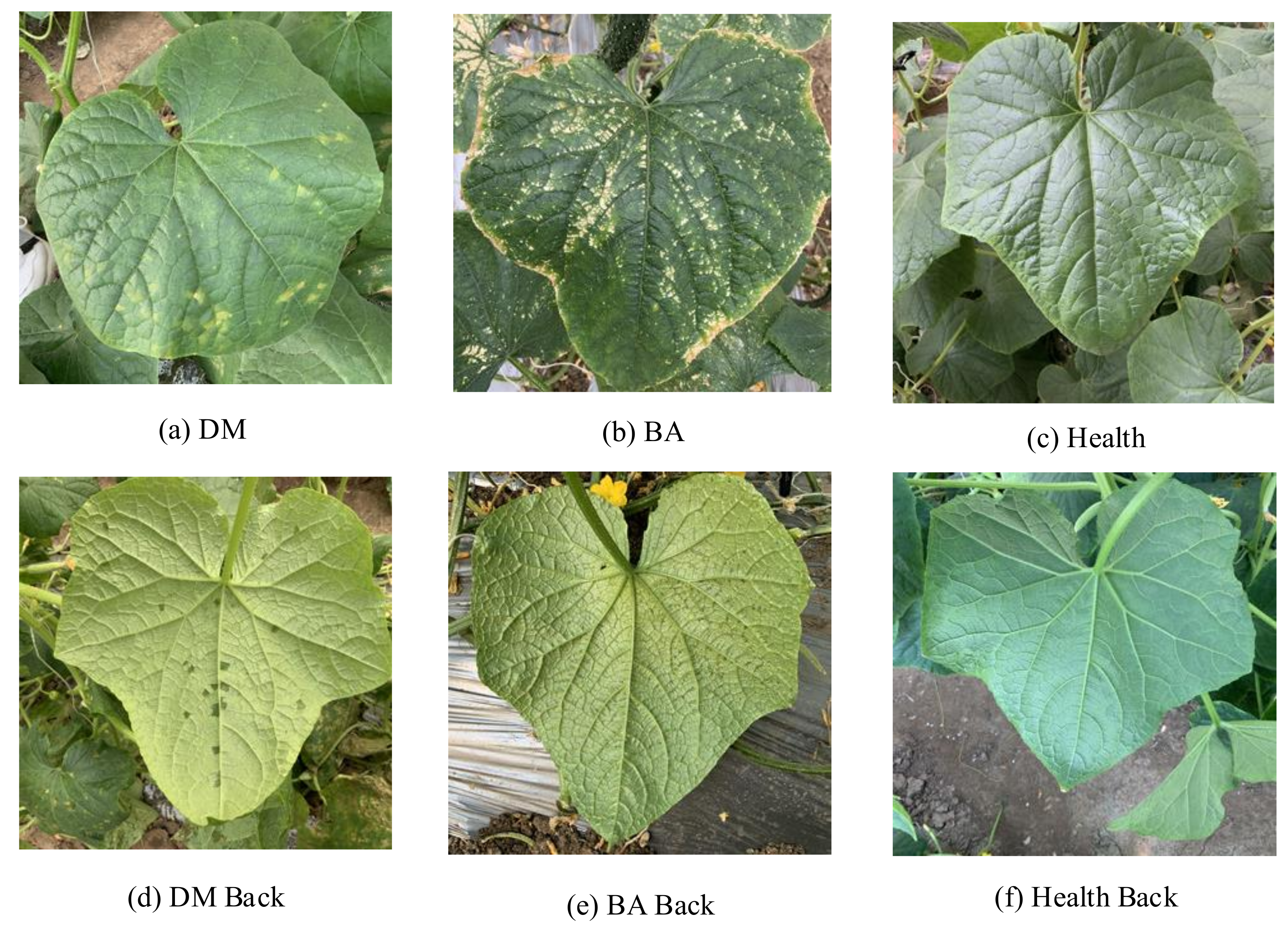
The cucumber dataset used in this paper was collected by mobile phones from October to November 2020 in Xiaotangshan National Precision Agriculture Research Demonstration Base in Beijing, with a total of 2542. Considering that the greenhouse smart device will inevitably capture the complex field background when collecting images, the images captured in this study all contain a field background. Due to the characteristics of bacterial angular leaf spot and downy mildew on the abaxial cucumber leaves only occurring in high humidity morning environments, images were collected between 7 am and 9 am. The images in the cucumber disease dataset can be divided into 6 categories (e.g., the backside of the downy mildew leaf (DM Back), the front side of the downy mildew leaf (DM), the backside of the bacterial angular spot leaf (BA Back), the front side of the bacterial angular spot leaf (BA), the backside of the healthy leaf (Health Back), and the front side of the healthy leaf (Health)), as shown in Figure 1. Because of the large differences between the symptoms on the adaxial and abaxial of cucumber leaves, the front side and backside of cucumber leaves are divided into two classes. The amount of data for each category is shown in Table 1. In this study, the dataset is randomly divided into the training set, test set, and validation set according to a ratio of 6:3:1.

Figure 1.
Sample images of the cucumber disease dataset (original image size:1024 × 1024): (a) The front side of the downy mildew leaf (DM). (b) The front side of the bacterial angular spot leaf (BA). (c) The front side of the healthy leaf (Health). (d) The backside of the downy mildew leaf (DM Back). (e) The backside of the bacterial angular spot leaf (BA Back). (f) The backside of the healthy leaf (Health Back).

Table 1.
Data quantities and categories of various classes in the cucumber disease dataset.
2.1.2. Random Data Enhancement
To improve the model’s training effect, random data enhancement is used to expand the data. Existing data enhancement usually augments the dataset to a fixed amount before training, but the over-fitting phenomenon can still occur when the number of training rounds increases. In this study, different data enhancement methods are randomly combined to enhance data in each iteration during training. Moreover, the parameters in these data enhancement methods are also randomly chosen in each epoch. In this manner, the data samples used in each training epoch are different, which avoids the over-fitting problem caused by the small amount of data and a large number of iterations. In addition, it can improve the model’s generalization ability and final classification accuracy.
In the cucumber disease classification task, the color of the disease spots is one of the important features of classification; thus, this task only uses the random combination of geometric transformation methods such as flip, rotation, clipping, deformation, and scaling to expand the dataset. Since the data generated by each epoch of the model are different, the amount of data used for model training is proportional to the number of the epoch. The data amount involved in training can be calculated by Equation (1), where is the amount of data in each epoch, is the total number of the data participated in the training process, and is the total number of training epochs.
2.2. Methods
2.2.1. Model Architecture
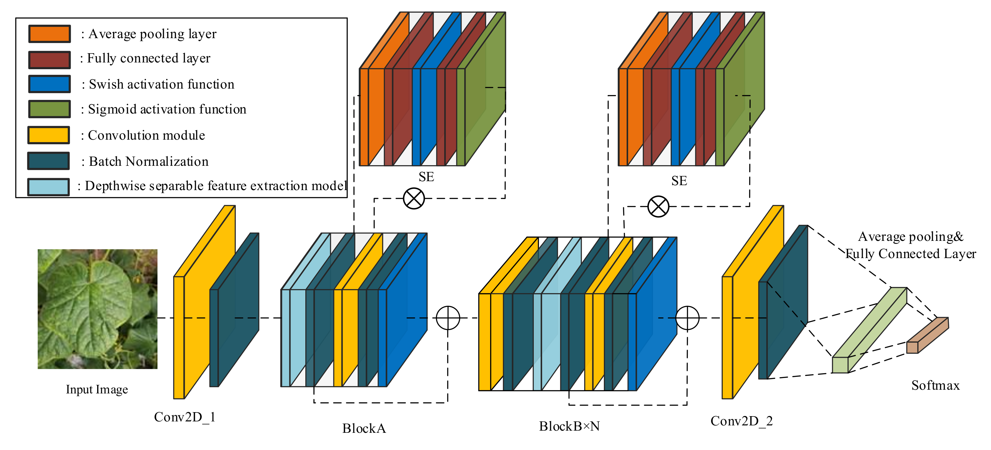
To obtain a suitable model for the cucumber disease classification task, we firstly built four models using the convolution feature extraction method. Then, the most suitable model was reconstructed by the addition feature extraction method. The basic structure of these models is shown in Figure 2, which is designed based on conventional convolution modules BlockA and BlockB. In this study, the structural complexity of the model is controlled by changing the number of BlockB. The four models’ detailed parameter settings are shown in Table 2.

Figure 2.
The structure of the cucumber disease classification model.
Table 2.
Parameter setting of each block in the model.
The structure of BlockA and BlockB is shown in Figure 3. BlockA and BlockB are mainly composed of a depthwise separable convolution module, a squeeze-and-excitation module (SE), and a conventional convolution module. One important difference between BlockA and BlockB is that BlockB initially uses a conventional convolution block to expand the number of channels in the feature map. It can help the model in obtaining more high-semantical features of disease spots. The conventional convolution module in BlockA and the second conventional convolution module in BlockB only fuse features obtained from SE, and it does not change the number of channels. At the same, to avoid the gradient divergence problem, a shortcut connection is used in the model to add feature maps extracted at different stages. The two blocks not only have lower computation and parameter amounts but also can guarantee the classification accuracy of the model. Thus, we used the two blocks to construct the cucumber disease classification model in this study.
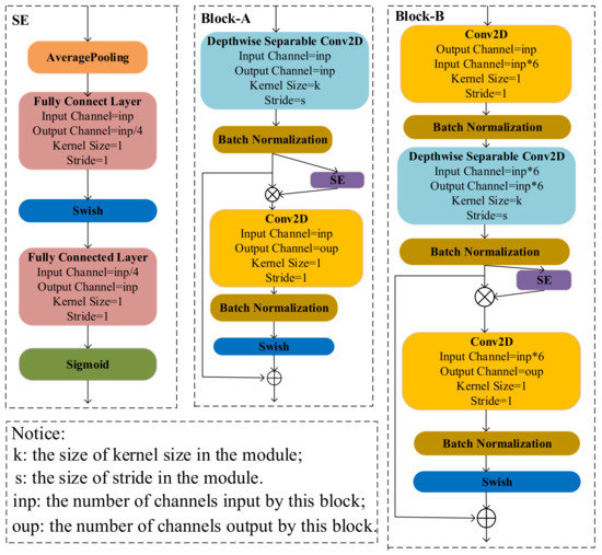
Figure 3.
The structure of blocks in the model.
In addition, batch normalization was used after each convolution module to improve the model’s training speed. The feature maps extracted from the multi-layers are sequentially sent to the convolution module and the batch normalization layer to speed up the model’s convergence speed. Then, the feature map is inputted into the average pooling layer and the fully connected layer and finally inputted into the softmax layer to obtain the probability of belonging to each category. Based on the final experimental results, Model2 (CNNLight) was chosen as the model structure for the task. CNNLight has a relatively small amount of parameters and computation amount. From the perspective of reducing computation amount, CNNLight reduces computational energy consumption. To further reduce the computational energy consumption of the model, this study used the additive feature extraction method to reconstruct CNNLight, and the reconstructed model ADDLight with lower computational energy consumption was the final model used in greenhouse edge devices.
2.2.2. Additive Feature Extraction Method
For the edge devices with limited battery capacity, using the additive feature extraction method can make these devices work longer [22]. The process of feature extraction can be regarded as measuring the similarity between the feature map and the feature extraction kernel. Thus, it is feasible to use addition instead of multiplication to calculate the distance of feature maps and feature extraction kernels. As shown in Figure 4a, the first normal form is used to calculate the cross-correlation between feature extraction kernels and feature maps. In this manner, the additive feature extraction method can be used to extract features from images. The forward propagation calculation formula of the additive feature extraction method is shown in Equation (2):
where is the kernel function of the model’s middle layers, d is the kernel size, is the number of the input channels, is the number of output channels, is the input feature map, H and W are the height and width of a feature map, respectively, and Y represents the extracted feature map.
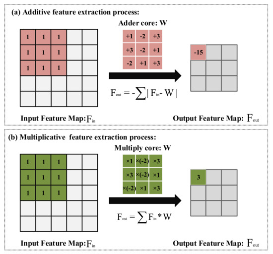
Figure 4.
Addition and multiplication feature extraction method: (a) The feature extraction process uses the addition method. (b) The feature extraction process using the multiplication method.
To solve the problem where the output of the added neural network is all negative, batch normalization was used to normalize the output. Since the additive feature extraction method uses an absolute value in the forward propagation function, the partial derivative of output feature map Y relative to convolution kernel F cannot be directly obtained in backpropagation. To solve this problem, this study used an L2 norm as the gradient calculation method. The calculation formula is shown in Equation (3).
The L2 norm is also used as the gradient calculation formula when solving the partial derivative of output feature map Y relative to input feature X. To avoid the gradient explosion problem caused by the deep network, the HT (HardTanh) function was used to truncate the derivation result. The calculation formula is shown in Equation (4). The final calculation formula of the partial derivative between output feature X and input feature Y is shown in Equation (5).
The similar output distribution between layers in the neural network is more conducive to the stability of network training. Hence, this study used a normalization operation after each layer of the neural network. For a given training batch , the formulation of batch normalization is stated in Equation (6):
where and are the learnable parameters, and and are the mean and variance of the output feature map, respectively.
In summary, the gradient calculation formula of the batch normalization layer in the adder neural network is shown in Equation (7).
Due to the large variance value of each layer in the model, the magnitude of the calculated partial derivatives will become smaller. To avoid gradient vanishment during training, the gradient of each layer is readjusted using the adaptive learning rate based on normalization. The gradient calculation formula of each layer is shown in Equation (8):
where is the update parameter amount for the l layer of the network, represents the global learning rate, represents the learning rate of the l layer, and is the gradient of the l layer. To keep the updated amount of the parameters in each layer consistent, this study adjusted the learning rate of each layer, and the adjustment’s calculation is shown in Equation (9):
where k is the number of elements in , and is a learnable hyperparameter.
2.2.3. Depthwise Separable Additive Feature Extraction Module
Our proposed model was designed based on depthwise separable convolution modules. Compared with conventional convolution modules, depthwise separable convolution modules have low parameters and calculation amounts [25].
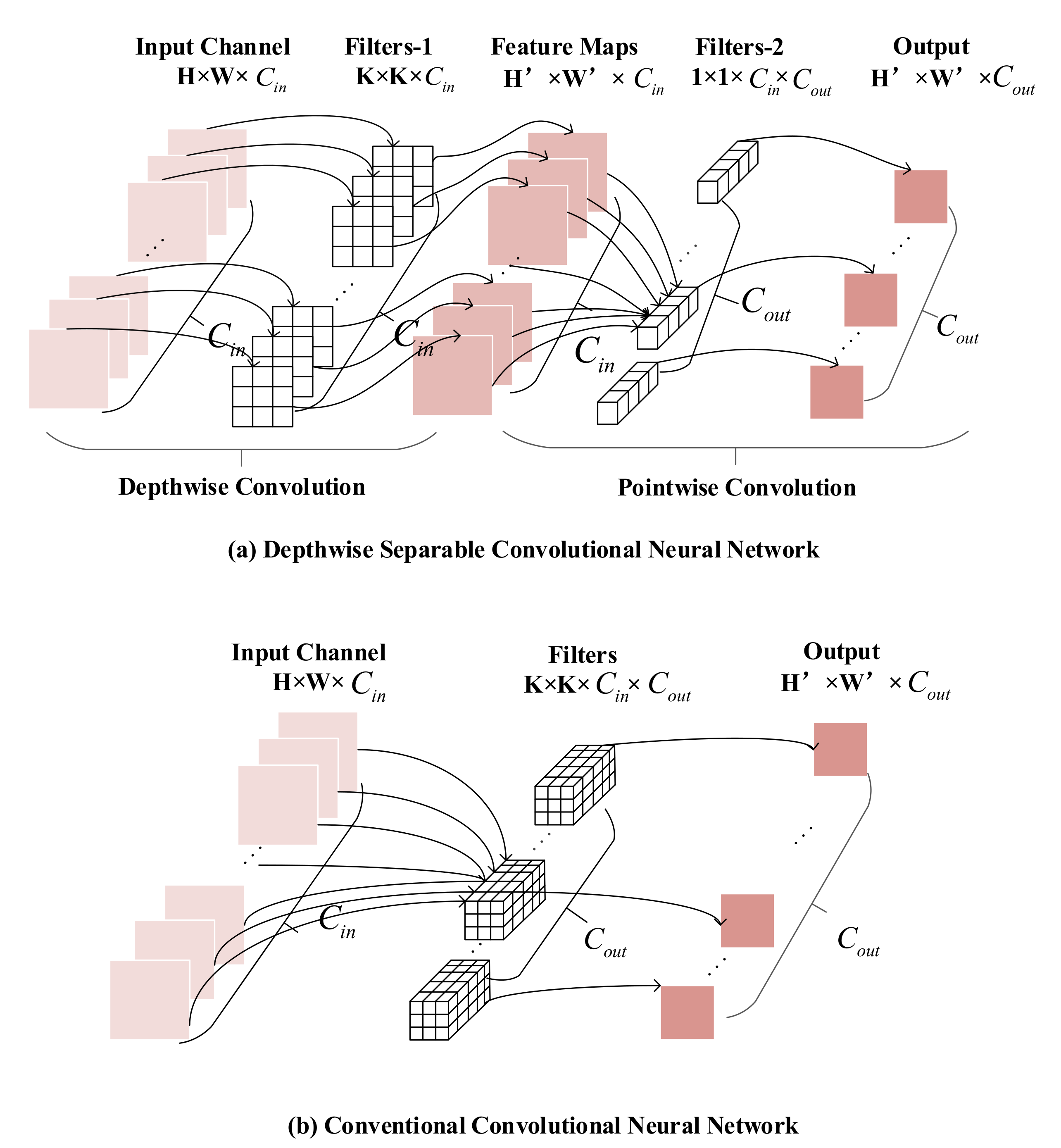
As shown in Figure 5, the depthwise separable convolution module divides the conventional convolution operation into two steps, as shown in Equations (10) and (11).
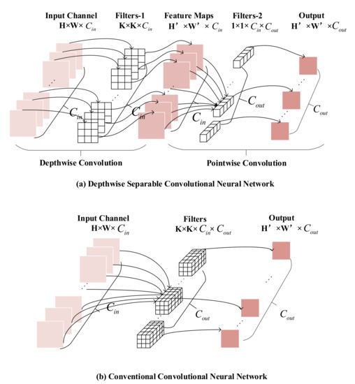
Figure 5.
Comparison of feature extraction process. (a) is the depthwise separable feature extraction process, (b) is the conventional convolution feature extraction process.
The first step is depthwise convolution, the number of channels in filters is one, and the number of filters is the same as the number of channels in the input feature map. The second step is pointwise convolution, which uses the convolution kernel with a kernel size of 1 to fuse feature maps in depth to obtain the final feature map. It is noticeable that the number of channels in filters is the same as the number of feature maps extracted from the previous step. It can be observed that the dimensions of feature maps extracted by the depthwise separable convolution module are consistent with that extracted by the conventional convolution module. The computation and parameter amounts of the depthwise separable convolution module and conventional convolution neural network are shown in Equations (12) and (13), respectively:
where K is the size of the convolution kernel, and are the length and width of an output feature map respectively, is the number of channels of the input feature map, and is the channel number of the output feature map. It can be observed that compared with the conventional convolution module, the depthwise separable convolution module reduces the computation amount and parameter number of the model to a large extent.
2.2.4. Additive Squeeze-and-Excitation Module
To improve the expression ability of important features in the feature map, Hu et al. [26] proposed using the squeeze-and-excitation module (SE) to adjust the feature weights of the channel. As Figure 3 shows, firstly, the input feature map is input into the average pooling layer and converted into a one-dimensional vector with the same length as the number of channels in the input feature map. Then, the vector is sequentially input into the two fully connected layers and a sigmoid activation function for weight learning. Finally, the input feature map multiplies the learning weight to obtain the weighted feature map. Many studies have shown that the SE module can improve classification accuracy degradation caused by the depthwise separable module [20,27]. To further reduce computational energy consumption, the feature extraction process involved in the SE module is reconstructed by the addition calculation method.
2.3. Evaluation Indicators and Experimental Environment
2.3.1. Evaluation Indicators
The evaluation indicators selected in this study can be divide into two groups. , , and are used to evaluate the diagnostic performance of the model. , , and are used to measure the calculation amount, parameter number, and calculation energy consumption of the model, respectively. The calculation formulas of , , and are shown in Equations (14)–(16):
where and represent the correct number of positive and negative samples, respectively. is the number of samples correctly predicted as positive samples, and are the number of negative samples predicted as positive and the number of positive samples predicted as negative samples, respectively.
measures the model’s complexity. It refers to the number of floating-point operations performed in complete forward propagation. The lower the , the lower the computation and execution time of the model. The is used to measure the parameter quantity of the model. The smaller the value, the lower the requirement of the model for device storage space. represents the energy consumed by the model to complete an image diagnosis. The parameters of the model constructed in this study are all 32-bit floating-point numbers. On a 45 nm 0.9 V device, the energy consumed by a 32-bit floating-point number addition and multiplication is 0.9 pJ and 3.7 pJ, respectively [28]. The lower the energy consumed by the model for disease classification, the longer the device will run after a single charge.
2.3.2. Experimental Parameters Setting
The adder neural network was constructed based on Pytorch and trained on CUDA 11.0. All experiments involved in this study were carried out in the Ubuntu 18.04.4 environment (processor: Intel Core I9 9820X; memory: 64 G; graphics card: GeForce RTX 2080Ti 11G DDR6).
To improve the convergence speed of the network and to reduce the negative influence of sample noise, the model used a combination of SGD and Momentum to update the weight during training [29]. We set the learning rate to 0.00001, momentum to 0.9, and weight decay to 0.0001. Due to the limitation of GPU memory, the batch size is set to 64, and the experiment is set 500 iterations.
3. Results
3.1. Comparison of Various Classification Models
To verify the effectiveness of the model structure constructed for the cucumber disease classification task, we compared the classification performance of five mainstream models (Efficientnet-B0 [30], ResNet18 [31], SqueezeNet [32], MobileNet-V3 [33], and VGG-16 [34]) with relatively fewer parameters. Their performance on the test dataset is shown in Table 3. The results clearly show that the five models have no significant difference in classification accuracy. VGG-16 and EfficientNet have the highest accuracy of 91.8%. Moreover, SqueezeNet has the lowest accuracy, which is 3.2% lower than VGG-16. While VGG-16 performed as well as EfficientNet, its model size was nearly 105-times larger than SqueezeNet, and its was approximately 38 times higher than EfficientNet. The classification accuracy of CNNLight is only 1.6% lower than that of VGG-16, but the model size is about 1070-times lower than that of VGG-16, and the computation amount is about 513-times lower than that of VGG-16. In terms of the model performance on the three indicators , , and , the results prove that CNNLight is more suitable for constructing a disease classification model. On the premise that the classification accuracy is only 0.13% lower than that of VGG-16 and the is only 15.30 MB, the of EfficientNet-B0 is 37.88% lower than that of MobileNet-V3.
Table 3.
Performance comparison of various classification models.
3.2. Comparison of Models Designed in This Study
To select the appropriate model complexity for the cucumber disease classification task, BlockA and BlockB (Figure 4) were used to build four models. The structure of all models in Table 4 is consistent with Figure 3, with the exception of only changing the number of BlockB. The network parameters of each model are shown in Table 2. It can be seen from the accuracy performance of Model1∼4 that the superposition of the BlockB module has limited improvement on model accuracy, but these models have a significant computation and model size reduction. These results also prove that different tasks have different requirements for model complexity. The classification accuracy of Model2 is 0.4% less than that of Model3, but its model size is about two times less than Model3. Considering the performance of models on three indicators, Model2 was selected as the disease diagnosis structure in this study.
Table 4.
Performance comparison of different model structures.
To further reduce the calculation amount of the model, we make some adjustments to the size of the input image. Among the models in Table 4, Model2-1 and Model2-2 have the same structure and parameter settings as Model2, but the input sizes of images is different. From the experimental results of Model2 and Model2-1, we can see that the two input sizes make little difference in the model’s classification accuracy. Although the classification accuracy of Model2-1 is 0.9% lower than that of Model2, the calculation amount of Model2-1 is nearly four-times lower than that of Model2. Based on experimental results, the input size of images is set as 112 for Model2.
3.3. Ablation Experiments
To analyze the effectiveness of each component in CNNLight, this paper conducts ablation experiments. As shown in Table 5, the random data enhancement strategy can improve the classification accuracy by 1.6%. The SE module has the highest improvement of classification accuracy on the model, which is 2.9%. This proves that the SE module can solve the problem of accuracy drops caused by depthwise separable convolution modules. In addition, using the shortcut connection can improve the classification accuracy of the model by 0.9%. The above experimental results demonstrate that these strategies promote the classification effect of the model on the cucumber disease classification task.
Table 5.
Ablation experiments for each module in CNNLight.
3.4. Comparison Experiment of ADDLight and CNNLight
To verify the advantages of the additive feature extraction method in edge devices, we experimented with CNNLight, the convolutional neural network with the same structure as ADDLight. The performance of the two models is shown in Table 6. The table shows that all the operations involved in ADDLight include addition. In CNNLight, the operation amount of addition and multiplication is equal. Although the calculation speed of different calculation methods differs depending on the CPU type, in general, the bit calculation speed is the fastest, followed by addition, multiplication, and division. On a device with the chip model Chipcon CC1010, the average clock cycle per addition is 1, and the average clock period per multiplication is 5 [35]. It can be observed that ADDLight performs a forward propagation twice as fast as CNNLight without any interference from other factors. The table also shows that ADDLight consumes about 96.1% less calculation energy for forward propagation than CNNLight. This means that greenhouse edge devices using ADDLight for the cucumber diseases classification task can work for a longer time. Although the classification accuracy of ADDLight is 1.1% lower than that of CNNLight, the accuracy of 89.1% can still meet the basic disease warning function.
Table 6.
Performance comparison of CNNLight and ADDLight.
3.5. Analysis of Model Performance on Each Category
Although ADDLight can greatly reduce the computational energy consumption of the model, classification accuracy is reduced compared to CNNLight. To further analyze the performance of ADDLight on various cucumber diseases, , , and of each category were calculated in this study. Each categories’ performance on the three indicators is shown in Table 7. Among the six categories, the values of and of five categories are up to 90%, which indicate that the model could more accurately predict the disease category of diseased leaves, but the of the backside of downy mildew leaf (DM Back) is relatively low, which is 83.78%. In addition, the of all categories is above 85%, and the F1-Score of the backside of bacterial angular spot leaf (BA Back) is up to 92.49%, which also proves that the model has a good balance effect in the value of and .
Table 7.
Classification performance of each category.
This study uses a confusion matrix to display the classification accuracy of each category to intuitively show the classification performance of ADDLight in each category. As shown in Figure 6, by comparing the misclassification results of the predicted labels and the real labels of each category, the reasons that affect the classification accuracy of the model can be further analyzed.
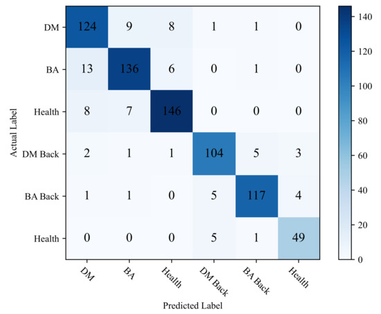
Figure 6.
Confusion matrix of ADDLight.
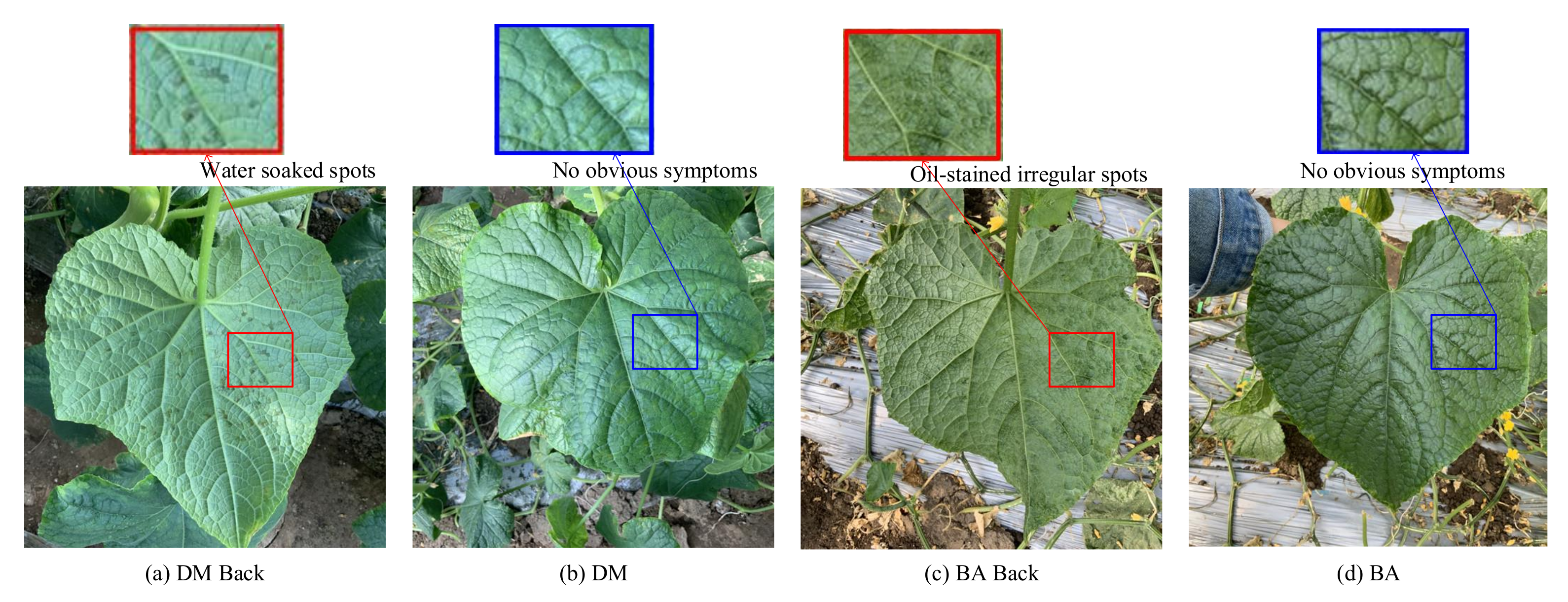
It can be seen from Figure 6 that the category of DM is easily misclassified into the category of BA and Healthy. The category of BA is easily misclassified into the category of DM and Health. Moreover, the category of Health is easy in being classified into BA and DM. This is mainly because the collection cycle of this dataset runs through the entire disease development period, and there are a large number of leaves at the disease initial stage. As shown in Figure 7, in the early stage of the disease, the disease spots of DW and BA are similar, and both of them have yellow punctuated spots. In addition, these disease spots of the two categories are small in the early disease stage; thus, it is easy to be confused with healthy leaves. In the early stage of the onset of downy mildew, the leaves on the back of the leaves will show water-soaked massive lesions, and bacterial angular spot disease will show oil-stained irregular round spots; thus, it is not easy to misclassify different types of leaves on the backside of the leaves. Distinct from the DW and BA, the symptoms of these disease lesions are very clear on DW Back and BA Back, even in the early disease stage. In the early stages of downy mildew, the leaves on the backside have water-soaked lesions, and the backside of the bacterial angular spot leaf shows oil-stained irregular round spots, which causes the classification accuracy on the two categories to be relatively higher.
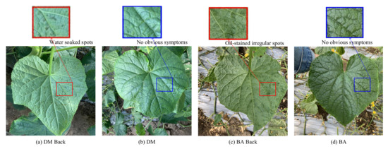
Figure 7.
Comparison of symptoms of different diseases: (a) The backside of downy mildew leaf with more water-soaked spots, (b) the front side of downy mildew leaf with no obvious symptoms in the early disease stage, (c) the backside of the bacterial angular leaf with more oil-stained irregular spots, and (d) the bacterial angular leaf with no obvious spots in the early disease stage.
4. Discussion
The question of how to design a model with high applicability on edge devices is an urgent problem in the agricultural engineering field. In this study, we used a depthwise separable feature extraction module and the squeeze-and-excitation module (SE) as basic modules to design a low energy-consumption model. The experimental results show that SE can make up for the deficiency of the low classification accuracy caused by the depthwise separable feature extraction module. Chen et al. [20] had the same idea as this study, but they only used the squeeze-and-excitation module to improve MobileNet’s classification performance rather than exploring a new combination structure. Their experimental results show that their proposed model with the depthwise separable convolution module and SE module is 1.15% higher than that of MobileNet-V2 on the rice dataset. In addition, the shortcut connection and channel expansion strategies are also used to improve classification accuracy. The ablation experiment shows good improvement for the two strategies. Both experiments of [36,37] were consistent with our experimental results.
To reduce the computational energy consumption of the model on edge devices, the proposed model is constructed by using an additive feature extraction method. The experimental results show that the adder disease classification model can greatly reduce energy consumption and prolong the working time of greenhouse devices, but the addition method impairs the classification performance of the model to a certain extent. Distinct from our method, De et al. [38] used the quantization method to compress the 32-bit parameters of the model into 4-bits in order to reduce the energy consumption and calculation amount of the model. The experimental results show that the quantization method can reduce the average energy consumption of the model by 6.5 times, and model quantization also reduces the classification accuracy of the model by about 1%. Although the experimental results proved that model quantization had little influence on classification accuracy, the model only used four categories of coffee-infected leaves for training and testing; thus, its conclusion was not very convincing in terms of classification accuracy. Similarly, Zhou et al. [19] quantified MobileNet’s weight tensor and activation function data from 32-bit to 8-bit. In their experiment, the quantization method reduced the model size of MobileNet V2 from 17.5 MB to 4.5 MB but resulted in a 1.1% loss in model classification accuracy. In this paper, the model size of the cucumber disease classification model we constructed in this paper is only 0.479 MB, and energy consumption was reduced to 96% by using the additive feature extraction method. Although the accuracy of the model is reduced by 1.1% compared with CNNLight, this model still has high applicability in real application scenarios. In future studies, we will continue to explore the main reasons affecting the classification accuracy of the adder cucumber disease classification model.
5. Conclusions
To improve the model’s applicability on edge devices and to extend the working time of the device, this study aims at constructing a low-energy-consumption additive cucumber disease classification model from the perspective of changing the feature extraction method and reducing computation amounts. The main achievements can be summarized as follows.
Firstly, we used the depthwise separable feature extraction module, the squeeze-and-excitation module, the short-cut connection strategy, and channel expansion strategy to design a lightweight cucumber disease classification model with good classification accuracy. The computational energy consumption of the model was reduced from the perspective of reducing the computation amount.
Secondly, the depthwise additive feature extraction and the additive squeeze-and-excitation modules were constructed to construct the disease classification model. Since the addition calculation has lower computational consumption than other operations, the model designed in this study also reduces computational energy consumption from the perspective of changing the calculation method.
Thirdly, compared with the convolutional neural network with the same structure, the computational energy consumption of the adder cucumber disease classification model is reduced by 96.1%. The experimental result shows that the model has high applicability for greenhouse edge devices. Although the final classification accuracy of the model is 1.1% lower than that of the convolutional neural network with the same structure, the classification accuracy of 89.1% can still meet the requirements of the cucumber disease warning task under complex environments.
Author Contributions
Conceptualization, C.L.; methodology, C.L.; software, C.L.; validation, H.W., C.Z., and X.H.; formal analysis, C.L.; investigation, C.L.; resources, C.Z. and H.W.; data curation, C.Z. and H.W.; writing—original draft preparation, C.L.; writing—review and editing, C.L.; visualization, S.L.; supervision, X.H., C.Z. and H.W.; project administration, C.L.; funding acquisition, H.W. and C.Z. All authors have read and agreed to the published version of the manuscript.
Funding
This research was funded by the National Natural Science Foundation of China (grant number 61871041), China Agriculture Research System of MOF, and MARA (grant number CARS-23-C06), Project of Agricultural Equipment Department of Jiangsu University (grant number 4111680005). The authors appreciate the funding organization for its financial support.
Institutional Review Board Statement
Not applicable.
Informed Consent Statement
Not applicable.
Data Availability Statement
The data presented in this study are available upon request from the corresponding author. The data are not publicly available due to the privacy policy of the authors’ Institution.
Acknowledgments
We thank all of the funders and all reviewers.
Conflicts of Interest
The authors declare no conflict of interest.
Abbreviations
The following abbreviations are used in this manuscript:
| DM | The front side of the downy mildew leaf; |
| BA | The front side of the bacterial angular spot leaf; |
| Health | The front side of the healthy leaf; |
| DM Back | The backside of the downy mildew leaf; |
| BA Back | The backside of the bacterial angular spot leaf; |
| Health Back | The backside of the healthy leaf; |
| SE | Squeeze-and-excitation module; |
| CPU | Central Processing Unit; |
| GPU | Graphic Processing Unit. |
References
- Yang, L.; Huang, B.; Mao, M.; Yao, L.; Niedermann, S.; Hu, W.; Chen, Y. Sustainability assessment of greenhouse vegetable farming practices from environmental, economic, and socio-institutional perspectives in China. Environ. Sci. Pollut. Res. 2016, 23, 17287–17297. [Google Scholar] [CrossRef] [PubMed]
- Chen, J.W.; Lin, W.J.; Cheng, H.J.; Hung, C.L.; Lin, C.Y.; Chen, S.P. A smartphone-based application for scale pest detection using multiple-object detection methods. Electronics 2021, 10, 372. [Google Scholar] [CrossRef]
- Ngugi, L.C.; Abdelwahab, M.; Abo-Zahhad, M. Tomato leaf segmentation algorithms for mobile phone applications using deep learning. Comput. Electron. Agric. 2020, 178, 105788. [Google Scholar] [CrossRef]
- Rao, D.; Krishna, M.; Ramakrishna, B. Smart ailment identification system for Paddy crop using machine learning. Int. J. Innov. Eng. Manag. Res. 2020, 9, 96–100. [Google Scholar]
- Chen, Y.; Liu, Z.; Zhang, Y.; Wu, Y.; Chen, X.; Zhao, L. Deep reinforcement learning-based dynamic resource management for mobile edge computing in industrial internet of things. IEEE Trans. Ind. Inform. 2020, 17, 4925–4934. [Google Scholar] [CrossRef]
- Khanramaki, M.; Asli-Ardeh, E.A.; Kozegar, E. Citrus pests classification using an ensemble of deep learning models. Comput. Electron. Agric. 2021, 186, 106192. [Google Scholar] [CrossRef]
- Zhou, J.; Li, J.; Wang, C.; Wu, H.; Zhao, C.; Wang, Q. A vegetable disease recognition model for complex background based on region proposal and progressive learning. Comput. Electron. Agric. 2021, 184, 106101. [Google Scholar] [CrossRef]
- Zhang, P.; Yang, L.; Li, D. EfficientNet-B4-Ranger: A novel method for greenhouse cucumber disease recognition under natural complex environment. Comput. Electron. Agric. 2020, 176, 105652. [Google Scholar] [CrossRef]
- Bateni, S.; Wang, Z.; Zhu, Y.; Hu, Y.; Liu, C. Co-optimizing performance and memory footprint via integrated cpu/gpu memory management, an implementation on autonomous driving platform. In Proceedings of the 2020 IEEE Real-Time and Embedded Technology and Applications Symposium (RTAS), Sydney, Australia, 21–24 April 2020; pp. 310–323. [Google Scholar]
- Wu, W.; Li, P.; Fu, X.; Wang, Z.; Wu, J.; Wang, C. GPU-based power converter transient simulation with matrix exponential integration and memory management. Int. J. Electr. Power Energy Syst. 2020, 122, 106186. [Google Scholar] [CrossRef]
- Zhou, R.; Kaneko, S.; Tanaka, F.; Kayamori, M.; Shimizu, M. Disease detection of Cercospora Leaf Spot in sugar beet by robust template matching. Comput. Electron. Agric. 2014, 108, 58–70. [Google Scholar] [CrossRef]
- Petrellis, N. Plant Disease Diagnosis Based on Image Processing, Appropriate for Mobile Phone Implementation. In Proceedings of the HAICTA, Kavala, Greece, 17–20 September 2015; pp. 238–246. [Google Scholar]
- Petrellis, N. Mobile application for plant disease classification based on symptom signatures. In Proceedings of the 21st Pan-Hellenic Conference on Informatics, Larissa, Greece, 28–30 September 2017; pp. 1–6. [Google Scholar]
- Hlaing, C.S.; Zaw, S.M.M. Model-based statistical features for mobile phone image of tomato plant disease classification. In Proceedings of the 2017 18th International Conference on Parallel and Distributed Computing, Applications and Technologies (PDCAT), Taipei, China, 18–20 December 2017; pp. 223–229. [Google Scholar]
- Sunny, S.; Gandhi, M.I. An efficient citrus canker detection method based on contrast limited adaptive histogram equalization enhancement. Int. J. Appl. Eng. Res 2018, 13, 809–815. [Google Scholar]
- Tiwari, V.; Joshi, R.C.; Dutta, M.K. Dense convolutional neural networks based multiclass plant disease detection and classification using leaf images. Ecol. Informatics 2021, 63, 101289. [Google Scholar] [CrossRef]
- Kamal, K.; Yin, Z.; Wu, M.; Wu, Z. Depthwise separable convolution architectures for plant disease classification. Comput. Electron. Agric. 2019, 165, 104948. [Google Scholar]
- De Ocampo, A.L.P.; Dadios, E.P. Mobile platform implementation of lightweight neural network model for plant disease detection and recognition. In Proceedings of the 2018 IEEE 10th International Conference on Humanoid Nanotechnology, Information Technology, Communication and Control Environment and Management (HNICEM), Baguio City, Philippines, 29 November–2 December 2018; pp. 1–4. [Google Scholar]
- Zhou, Z.; Song, Z.; Fu, L.; Gao, F.; Li, R.; Cui, Y. Real-time kiwifruit detection in orchard using deep learning on Android™ smartphones for yield estimation. Comput. Electron. Agric. 2020, 179, 105856. [Google Scholar] [CrossRef]
- Chen, J.; Zhang, D.; Suzauddola, M.; Nanehkaran, Y.A.; Sun, Y. Identification of plant disease images via a squeeze-and-excitation MobileNet model and twice transfer learning. IET Image Process. 2021, 15, 1115–1127. [Google Scholar] [CrossRef]
- Rajbongshi, A.; Sarker, T.; Ahamad, M.M.; Rahman, M.M. Rose Diseases Recognition using MobileNet. In Proceedings of the 2020 4th International Symposium on Multidisciplinary Studies and Innovative Technologies (ISMSIT), Istanbul, Turkey, 22–24 October 2020; pp. 1–7. [Google Scholar]
- Chen, H.; Wang, Y.; Xu, C.; Shi, B.; Xu, C.; Tian, Q.; Xu, C. AdderNet: Do we really need multiplications in deep learning? In Proceedings of the Proceedings of the IEEE/CVF Conference on Computer Vision and Pattern Recognition, Seattle, WA, USA, 13–19 June 2020; pp. 1468–1477. [Google Scholar]
- Courbariaux, M.; Bengio, Y.; David, J.P. Binaryconnect: Training deep neural networks with binary weights during propagations. Adv. Neural Inf. Process. Syst. 2015, 28, 3123–3131. [Google Scholar]
- Hubara, I.; Courbariaux, M.; Soudry, D.; El-Yaniv, R.; Bengio, Y. Binarized neural networks. Adv. Neural Inf. Process. Syst. 2016, 29, 4107–4115. [Google Scholar]
- Han, S.; Mao, H.; Dally, W.J. Deep compression: Compressing deep neural networks with pruning, trained quantization and huffman coding. arXiv 2015, arXiv:1510.00149. [Google Scholar]
- Hu, J.; Shen, L.; Sun, G. Squeeze-and-excitation networks. In Proceedings of the IEEE Conference on Computer Vision and Pattern Recognition, Salt Lake City, UT, USA, 18–22 June 2018; pp. 7132–7141. [Google Scholar]
- Chao, X.; Hu, X.; Feng, J.; Zhang, Z.; Wang, M.; He, D. Construction of apple leaf diseases identification networks based on xception fused by SE module. Appl. Sci. 2021, 11, 4614. [Google Scholar] [CrossRef]
- Horowitz, M. 1.1 computing’s energy problem (and what we can do about it). In Proceedings of the 2014 IEEE International Solid-State Circuits Conference Digest of Technical Papers (ISSCC), San Francisco, CA, USA, 9–13 February 2014; pp. 10–14. [Google Scholar]
- Liu, C.; Belkin, M. Accelerating sgd with momentum for over-parameterized learning. arXiv 2018, arXiv:1810.13395. [Google Scholar]
- Tan, M.; Le, Q. Efficientnet: Rethinking model scaling for convolutional neural networks. In Proceedings of the International Conference on Machine Learning PMLR, Long Beach, CA, USA, 9–15 June 2019; pp. 6105–6114. [Google Scholar]
- He, K.; Zhang, X.; Ren, S.; Sun, J. Deep residual learning for image recognition. In Proceedings of the IEEE Conference on Computer Vision and Pattern Recognition, Las Vegas, NV, USA, 26 June–1 July 2016; pp. 770–778. [Google Scholar]
- Zhang, X.; Zhou, X.; Lin, M.; Sun, J. Shufflenet: An extremely efficient convolutional neural network for mobile devices. In Proceedings of the IEEE Conference on Computer Vision and Pattern Recognition, Salt Lake City, UT, USA, 18–23 June 2018; pp. 6848–6856. [Google Scholar]
- Howard, A.; Sandler, M.; Chu, G.; Chen, L.C.; Chen, B.; Tan, M.; Wang, W.; Zhu, Y.; Pang, R.; Vasudevan, V.; et al. Searching for mobilenetv3. In Proceedings of the IEEE/CVF International Conference on Computer Vision, Seoul, Korea, 27–28 October 2019; pp. 1314–1324. [Google Scholar]
- Simonyan, K.; Zisserman, A. Very deep convolutional networks for large-scale image recognition. arXiv 2014, arXiv:1409.1556. [Google Scholar]
- Gura, N.; Patel, A.; Wander, A.; Eberle, H.; Shantz, S.C. Comparing elliptic curve cryptography and RSA on 8-bit CPUs. In Proceedings of the International Workshop on Cryptographic Hardware and Embedded Systems, Cambridge, MA, USA, 11–13 August 2004; Springer: Berlin/Heidelberg, Germany, 2004; pp. 119–132. [Google Scholar]
- Liu, T.; Chen, M.; Zhou, M.; Du, S.S.; Zhou, E.; Zhao, T. Towards understanding the importance of shortcut connections in residual networks. Adv. Neural Inf. Process. Syst. 2019, 32, 7892–7902. [Google Scholar]
- Zhu, A.; Liu, L.; Hou, W.; Sun, H.; Zheng, N. HSC: Leveraging horizontal shortcut connections for improving accuracy and computational efficiency of lightweight CNN. Neurocomputing 2021, 457, 141–154. [Google Scholar] [CrossRef]
- De Vita, F.; Nocera, G.; Bruneo, D.; Tomaselli, V.; Giacalone, D.; Das, S.K. Quantitative analysis of deep leaf: A plant disease detector on the smart edge. In Proceedings of the 2020 IEEE International Conference on Smart Computing (SMARTCOMP), Bologna, Italy, 14–17 September 2020; pp. 49–56. [Google Scholar]


Publisher’s Note: MDPI stays neutral with regard to jurisdictional claims in published maps and institutional affiliations. |
© 2022 by the authors. Licensee MDPI, Basel, Switzerland. This article is an open access article distributed under the terms and conditions of the Creative Commons Attribution (CC BY) license (https://creativecommons.org/licenses/by/4.0/).