Abstract
Chestnut blight is the major disease of chestnuts (Castanea spp.) cultivated worldwide for the production of edible nuts. The disease is caused by the pathogenic fungus Cryphonectria parasitica, which infects trees by means of airborne propagules penetrating through fresh wounds on stems and branches. The aims of this study were to (I) assess the temporal propagule deposition patterns of C. parasitica in the Alpine district of North Western Italy, (II) test and model the effects of seasonality and climate on the above patterns, and (III) investigate the spatial distribution of propagule deposition at the within-site scale. A two-year-long spore trapping experiment was conducted in three chestnut orchards. Approximately 1300 samples were collected and processed with a species-specific qPCR assay to quantitatively assess the propagule deposition of C. parasitica. Results showed that C. parasitica can release propagules all over the year, though with significant seasonal peaks in the spring and fall (p < 0.05). Large propagule loads were significantly correlated (p < 0.05) with an increasing number of rainy days of the week (days providing 1–10 mm/day of water). Models predicting periods at high risk of infection based on climate and seasonality were fitted and successfully validated (p < 0.05).
1. Introduction
Chestnuts (Castanea spp.) are multipurpose tree species grown in orchards for the production of edible nuts or in forest stands to retrieve timber for various uses [1]. Moreover, chestnut trees provide relevant ecosystem services and allow for the sustainment of local economies in countryside areas, where agroforest systems play key roles in land management and social well-being [2,3]. Chestnut nuts are highly appreciated for their nutritional, nutraceutical, and organoleptic properties, and they feed a global export market of several hundred million dollars [4,5,6,7]. Not surprisingly, there has been a renewed interest in the chemical, biological and sensory characterization of nuts from different cultivars of the main chestnut species grown for fruit production, namely Castanea sativa Mill., C. crenata Sieb. et Zucc., C. mollissima Blume, and hybrids [8,9,10,11].
Notwithstanding the promising perspectives foreseen at the global scale, the cultivation of chestnuts in many regions is threatened by the onset or resurgence of emerging or endemic diseases. Some of these diseases can hamper the productivity of chestnut orchards and cause significant economic losses, but they do not lead to tree mortality. This is the case, for instance, of nut rots caused by fungal pathogens including Ciboria batschiana (Zopf) N.F. Buchw., Gnomoniopsis castaneae Tamietti, Sirococcus castaneae (Prill. and Delacr.) J.B. Mey., Senn-Irlet, and T.N. Sieber, and others (see Lione et al., 2019, [12] and the literature therein). Other diseases can trigger chestnut decline (e.g., foliar diseases) or even result in tree mortality (e.g., root rots), but such phenomena are generally limited in time and space or are associated with a preexisting state of environmental or age-related stress of the host [13]. Conversely, chestnut trees are susceptible to other fungal and fungus-like pathogens whose effects are often detrimental due to their establishment and spread abilities and to their virulence, often resulting in high mortality rates. The above pathogens include the causal agents of the “ink disease”, the chromistan Phytophthora cambivora (Petri) Buisman and P. cinnamomi Rands, and the fungus Cryphonectria parasitica (Murrill) M.E. Barr, which causes chestnut blight [13]. Though ink disease and chestnut blight are both classified as major diseases of chestnuts, the latter is probably the most relevant because of its impact on tree mortality, economic losses, and ecosystem degradation [13]. Cryphonectria parasitica was inadvertently introduced to North America from Asia during the earliest 1900s and then from North America to Europe in the late 1930s [14]. In North America, the pathogen spread over 3.6 million ha at an average rate of 30 km/year, killing approximately 3.5 billion trees and causing the functional extinction of the local species C. dentata in about 50 years [13]. In Europe, the effects of C. parasitica were less destructive than in North America, despite the substantial impact it had on the native C. sativa in orchards and forest stands [13]. Cryphonectria parasitica is a parasite that infects hosts by means of propagules (i.e., sexual spores or asexual conidia) penetrating fresh wounds or cracks exposing the cambial tissue of stems, branches, or twigs [14]. Hail wounds have recently been documented as important infection courts for the pathogen [15]. Other minor infection pathways involve galls abandoned by the insect pest Dryocosmus kuriphilus Yasumatsu or tissues weakened by natural disturbances (e.g., fires) serving as entry points for the propagules of C. parasitica [14]. Once the mycelium has grown, compromising the cambium and the bark, early symptoms of chestnut blight occur. Such symptoms may be variable depending on the virulence of C. parasitica strains infecting the host. Virulent strains of C. parasitica can rapidly colonize the cambium, causing lightly sunken necrotic lesions associated with the appearance of visible reddish areas. Lesions progress towards bark cankers that may result in the death of the upper portion of the infected stem or branch. The high severity of chestnut blight results in foliar, flower, and branch wilting, crown transparency, and (eventually) the death of entire crown portions or the whole tree. These symptoms are more pronounced when the diameter of woody organs is small and the bark is thin. However, some cankers may be less severe and allow the host to react by callousing the lesions. In this case, the stem or branch is able to survive. It is acknowledged that strains of C. parasitica associated with this milder type of canker display a reduced virulence due the presence of a mycovirus (Cryphonectria hypovirus 1—CHV1, a member of the species Alphahypovirus cryphonectriae) [14]. CHV1 present in the cytoplasm of a so-called hypovirulent strain can be transmitted to a virus-free (i.e., virulent) strain of C. parasitica via hyphal anastomoses, provided that the strains are vegetatively compatible, although CHV1 transmission can rarely occur even between vegetatively incompatible strains [14,16]. This mechanism has been employed to develop a biological control strategy against C. parasitica that depends on the inoculation of hypovirulent strains in close proximity of lesions caused by virulent ones. Once CHV1 infection occurs, the virulent strain is weakened and turns into a hypovirulent one, hence favoring a gradual recovery of the host tree [14,17]. The constraints of this control method are related to the difficulties in finding an adequate number of hypovirulent strains that are vegetatively compatible with most of the virulent ones present within a given site [14,16,17]. Moreover, the implementation of this control strategy is challenging, and it may take one or more decades to show some efficacy [17,18]. A complementary control strategy is based on the removal of branches with severe blight symptoms while leaving those with mild lesions (probably harboring hypovirulent strains). Hence, hypovirulent strains of C. parasitica are expected to freely sporulate and spread naturally in the orchard. However, CHV1 cannot be spread through sexual spores, and the percentage of the conidia of a hypovirulent strain carrying CHV1 has been reported to vary between 0 and 100% depending on the strain [19,20,21]. Since chemical therapy and other post-infection control strategies are not recommended due to their limited efficacy, most of the current practices to thwart chestnut blight hinge on preventive measures [13]. In particular, avoiding or reducing injuries on stems and branches is deemed an adequate approach to minimize the risk related to infections caused by C. parasitica [13,15]. Nonetheless, the ordinary management of chestnut orchards requires operations that imply, or are likely to imply, “inevitable” or “collateral” wounds. Inevitable injuries occur during pruning, topping, and grafting, while collateral wounds may occur during mechanical weeding, fruit collection, and whenever vehicles, machines, or tools result in injuries to trees [22,23]. In both cases, operating in orchards when the abundance of airborne propagules of C. parasitica is low might reduce the risk of infection. Therefore, unravelling the temporal patterns of the propagule deposition of C. parasitica, detecting the presence of seasonal trends, and investigating which climatic factors could be related to the release of airborne inoculum may be pivotal to predict when the risk of infection is high and fine-tune the calendar of in-field operations accordingly [24,25].
The spatial patterns of propagule deposition may convey information that could aid planning in-field operations in advance, especially prior to the establishment of the crop (e.g., define the plant density of the orchard) [26,27]. These aspects are clearly important in agriculture under an applied perspective, but they can also provide relevant insights to elucidate biological, ecological, and epidemiological traits of C. parasitica. For instance, assessing the spatial distribution of the propagule loads may offer some clues about the prevalence of either the sexual or the asexual reproduction strategy [27].
Based on the above-described premises, it is not surprising that aerobiological studies aimed at assessing the propagule deposition patterns of relevant plant pathogens of crops and investigating the underlying environmental factors are on the rise [28]. For instance, some specific studies targeting chestnut pathogens including C. parasitica [29] and G. castaneae [27] have already been published. However, propagule deposition patterns and the underlying relations with climatic factors may be highly variable depending on the geographic area [15,27,30]. To date, in Europe, the temporal propagule deposition of C. parasitica has only been investigated in a single location in close proximity to the Atlantic Ocean, in the plain areas of Western France [29], and no information is available for other areas of Europe, including the Alpine region. In addition, the spatial patterns of the propagule deposition of C. parasitica are still largely unknown.
In this study, a two-year-long aerobiological experiment was set up by combining a passive spore trap technique, a quantitative polymerase chain reaction (qPCR) assay to quantify the propagule loads of C. parasitica, and statistical approaches for data processing and interpretation. The main aims of the study were to (I) assess the temporal patterns of the propagule deposition of C. parasitica in orchards of the Alpine district of North Western Italy, (II) test and model the effects of seasonality and climate on the above patterns, and (III) unravel the spatial distribution of the propagule deposition at the within-site scale.
2. Materials and Methods
2.1. Study Sites
Three sites were chosen to host a two-year-long spore trapping experiment aimed at assessing the propagule deposition patterns of Cryphonectria parasitica. These sites were located at San Giorio di Susa (latitude 45.1196°, longitude 7.1852°, elevation 540 m a.s.l.), Peveragno (44.3261°, 7.5862°, 605 m), and Gaiola (44.3358°, 7.3914°, 823 m), hereafter indicated as either training or evaluation sites (TS or ES) with the acronyms TS1 (San Giorio di Susa,) TS2 (Peveragno), and ES (Gaiola), respectively. All study sites hosted mature/old-grown chestnut orchards, with mean diameters at breast height ranging from 46 to 67 cm and tree densities of between 75 and 107 plants/ha. Orchard extension covered 4 ha surrounded by other stands where chestnut was the most abundant species. The choice of these sites was based on previous studies reporting the extensive presence of chestnut blight in the surroundings [15,31]. Moreover, each study site was surveyed to verify the presence of chestnut blight symptoms including visible cankers on stems, branches, shoots, and twigs, as well as fruiting bodies of C. parasitica appearing as stromata with colors ranging from yellow to red on the bark surface of living trees [14]. A total of 10 symptomatic chestnut branches and shoots per site were collected and processed as described by Lione et al. (2020) [15] to attempt the microbial isolation targeting C. parasitica. The identification of the pathogen was conducted by observing the morphological characteristics of the isolates, as reported by Lione et al. (2020) [15]. Further information about the study sites was reported in the study by Lione et al. (2021) [27], in which the same orchards were used to conducts a similar experiment targeting the propagule deposition patterns of Gnomoniopsis castaneae.
2.2. Spore Trapping Experiment
To monitor the propagule loads of C. parasitica, 14 spore trap devices per study site were placed along a permanent linear transect of 130 m, equidistant from each other every 10 m. As described by Lione et al. (2021) [27], each spore trap consisted of a passive device made with a sterile disc of Whatman® filter paper (15 cm diameter) fixed to the bottom of a Petri plate of the same diameter. Petri plates were drilled to obtain 4 holes of approximately 0.5 cm in diameter in order to allow for water drainage and prevent the soaking of the filter paper during rainfalls. The same holes were used to tie a sterile copper cable aimed at fastening the filter paper to the Petri plate. Petri plates were placed horizontally at 1.50 m above the ground level by using a tripod anchored to the soil, with the filter paper oriented upwards to capture the propagule loads. Prior to its in-field exposure, filter paper was imbibed with a solution of a 4X TE buffer (40 mM Tris-HCl, and 4 mM EDTA at pH 8.0, with a total volume of 20 mL per trap), with the aim of: I) allowing for the adhesion of the propagules to the filter paper and II) preventing DNA degradation and fungal spore germination [32,33]. The spore traps were protected from direct sunlight by the canopy, so the filter paper could maintain a sufficient wetness during the exposure time. The position of all spore traps deployed along the transect was labelled with increasing integers from 1 to 14. During a timeframe of two years (from 15 Ocotber 2013 to 27 Ocotber 2015), 35 and 24 samplings were conducted in the TS and ES sites, respectively, on average every 21 days (sd = 8 days). Samplings were less frequent in ES than in TS sites because data from ES were used to validate results and models obtained from TS sites (see sections below). At each sampling, the filter papers exposed in the field were replaced with new ones prepared as previously described. Old filter papers were moved into a Falcon® tube, immediately transported to the laboratory, and stored at a constant temperature of −80 °C.
2.3. Assessment of the Analytical Specificity and Sensitivity of the qPCR Assay
Spore traps collected from the study sites were analyzed with a qPCR assay similar to that reported by Lione et al. (2021) [27] but optimized to quantify the propagule deposition of C. parasitica. The first phase of the method optimization involved the assessment of the analytical specificity of the primers used to target C. parasitica, namely Cp-F4 (5′-GATACCCTTTGTGAACTTATAA-3′) and Cp-R3 (5′-GGGGAGAAGGAAGAAAATC-3′) [34]. The second phase was oriented to appraise the analytical sensitivity of the qPCR assay. Both phases are described below.
To verify the specificity of the amplification of the Cp-F4 and Cp-R3 primers, samples of DNA from 25 non-target species of fungi were used as template to run a qPCR with the primers. DNA samples of non-target species were obtained from the 25 fungal isolates obtained from environmental samples in chestnut stands during a previous study conducted by Lione et al. (2021) [27] (Table S1). Isolates were grown for 7 days in malt extract broth (2%) and stored at a temperature of 25 °C for 7 days prior to perform the DNA extraction, which was carried out by using the EZNA® Stool DNA Kit (Omega Bio-Tek, USA) on freeze-dried mycelium previously processed as reported by Lione et al. (2021) [27].
To carry out the qPCR, a 96-well plate was used with a Connect™ Real-Time PCR Detection System device (Bio-Rad Laboratories), each filled with: DNA (1 μL at a concentration of 10 ng/μL), SsoAdvanced Universal SYBR Green Supermix (5 μL; Bio-Rad Laboratories), primer Cp-F4 (0.2 μL), primer Cp-R3 (0.2 μL at 3 μM), and sterile water (3.6 μL). The positive and negative controls used to run the qPCR were a DNA extract obtained from the Italian isolate of C. parasitica 5183 L2d (origin: Aosta Valley, obtained from the activities related to the MONGEFITOFOR project) and sterile water, respectively. Two technical replicates were included for both samples and controls. The protocol of the qPCR comprised the following steps: 2 min at 98 °C, 40 cycles of 15 s at 95 °C, and 30 s at 60 °C. Data related to the fluorescence and amplification threshold cycle (Ct) were obtained from the qPCR instrument at the completion of the extension phase. An analysis of the melting curves was conducted by setting the following parameters: a temperature gradient of 65–95 °C with steps of 0.5 °C and plate reading every 5 s.
In order to assess the analytical sensitivity of the qPCR assay, the limits of detection (LOD) and quantification (LOQ) of the Cp-F4 and Cp-R3 primers were determined as described below. A ten-fold serial dilution of a DNA extract of C. parasitica 5183 L2d was prepared in two different matrices, starting from 20 ng·μL−1 and proceeding until the final concentration of 2 fg·μL−1 was reached. For the first matrix (water matrix), the DNA of C. parasitica was diluted in MilliQ sterile water to determine the LOD without the presence of non-target DNA. For the other matrix (environmental matrix), DNA was extracted from a filter paper exposed in the field. This environmental DNA sample, free from C. parasitica DNA, was used in order to assess whether the LOD could be affected by non-target DNA. Therefore, a ten-fold serial dilution of the C. parasitica 5183 L2d DNA extract was prepared in this environmental DNA matrix. For both matrices, dilutions were made by using six technical replicates, including additional two replicates for the negative controls (sterile MilliQ water). qPCR reactions were conducted to generate the standard curve to calculate LOD and LOQ values for each matrix, as reported by Desimoni and Brunetti (2015) [35].
LOD and LOQ were also determined by extracting DNA from the filter paper of the traps. The same DNA allowed us to generate the standard curve needed to process the spore traps collected at each sampling. These operations were conducted on 21 sterile spore traps (7 traps × 3 replicates) imbibed with a water suspension of C. parasitica conidia (1 mL) under a biological hood. The suspension was prepared by collecting conidia produced by isolate 5183 L2d grown on PDA plates incubated at 25 °C for 10 days. Conidia were suspended in sterile water and counted with an optical microscope (200× magnification), with the support of a Bürker chamber. Ten-fold serial dilutions ranging from 10 to 107 conidia·mL−1 were performed. The above concentrations were used separately to wet each set of spore trap replicates, from which a subsequent DNA extraction was carried out. A further qPCR was run as previously described to process these DNA extracts and build the standard curve to be used as reference for the quantification of the propagule deposition of C. parasitica in the field. The standard curve allowed us to associate the initial DNA concentrations and the corresponding number of conidia with the Ct value at which the C. parasitica DNA was amplified above a threshold baseline.
2.4. Spore Traps Processing and Propagule Deposition Quantification
Samples of filter paper collected in the study sites were processed to quantify the propagule deposition of C. parasitica by using the method reported by Lione et al. (2021) [27] and the optimized qPCR described in the previous section. In brief, each paper disc exposed in the field was cut into thin strips, stored in a sterile 50 mL Falcon tube, immersed in a warm TE buffer, vortexed (5 min), and then centrifuged (875× g and 25 °C for at least 60 min) until the pellet (putatively containing spores/conidia) could be separated from the supernatant. The pellet was then resuspended in sterile water, moved into Eppendorf® tubes (2 mL), homogenized with laboratory equipment and resuspended in a CTAB extraction buffer [27], vortexed, and then iteratively frozen at −196 °C and heated twice at a temperature of 65 °C for 2 min. The following steps included the addition of the same volume of chloroform/isoamyl alcohol (24:1), centrifugation (12,300× g and 25 °C for 10 min) and the separation of the upper phase. From that phase, the precipitation of DNA was obtained through the addition of cold isopropanol followed by a further centrifugation (15,366× g and 25 °C for 5 min). Successively, the supernatant was removed and the pellet was treated with ethanol (70%) and suspended in a TE buffer (30 μL) after drying (65 °C).
The optimized qPCR assay described in the previous section was used to process the samples collected from the three study sites. The qPCR outcomes were retained if the following conditions were met: (I) the standard curve slope ranged from 2.9 to 3.5, (II) the R2 of the standard curve was over 0.97, and (III) the efficiency E was in the range of 0.90–1.10 [27]. The absolute quantification of the propagule loads of C. parasitica deposited onto each spore trap was carried out by intersecting the Ct obtained from spore traps to the standard curve obtained in the laboratory and based on given concentrations of conidia (see previous section). The Biorad CFX Manager™ software was used to analyze melting curves and to inspect those obtained from positive samples to confirm the correspondence to C. parasitica specific melting curves. The equations reported in the supplementary files of Lione et al. (2021) [27] were used to convert the absolute quantification of C. parasitica (sexual spores/conidia per μL) into the corresponding deposition rate of airborne inoculum (DR, in propagules·m−2·h−1).
A further PCR reaction performed with the universal eukaryotic primer set ITS1/ITS4 [36] was carried out to verify the absence of C. parasitica DNA in samples showing no amplification curves. The PCR mix included 6.25 μL of DNA (diluted 1:10), 0.025 U of Taq polymerase (GoTaq® G2 DNA Polymerase, Promega, Madison, WI, USA), 0.5 μM of the different primers, 200 μM of every deoxynucleotide triphosphate (dNTP), and 5 μL of the 5X buffer (overall volume—25 μL). The series of steps conducted for the described PCR comprised a denaturation step of 3 min at 94 °C, 35 cycles of 30 s each at 94 °C, 30 s at 54 °C, 45 s at 72 °C, and a final elongation step of 10 min at 72 °C. A negative (sterile water) and a positive (C. parasitica DNA of isolate 5183 L2d) control were incorporated as well. The amplification products were observed with a GelRed™ (Biotium; 1 μg·mL−1) on agarose gel (1% w/v) in the TBE buffer by setting the electrophoresis as reported by Lione et al. (2021) [27].
2.5. Collection and Pre-Processing of Variables
Variables potentially related to the propagule deposition rates of C. parasitica were obtained and pre-processed prior to a further statistical analysis as reported by Lione et al. (2021) [27].
Temporal variables included the calendar month (MS) of each sampling and its corresponding meteorological season (SM). Climatic data were retrieved on a daily basis by placing weather stations at all study sites (Onset Hobo® series) equipped with hardware able to measure and record: mean, maximum and minimum temperatures (tmean, tmax, and tmin, respectively; °C); mean, maximum and minimum relative humidity (rhmean, rhmax, and rhmin, respectively; %); and total precipitations (p, mm). From this list, a set of additional climatic variables was calculated, including the growing degree days (°C) with thresholds 0 and 5 °C (gdd0, ggd5) and the number of days with over 0, 1, 2, 5, 10, 15, 20, 25, and 30 mm of precipitations (ndp0, ndp1, ndp2, ndp5, ndp10, ndp15, ndp20, ndp25, and ndp30, respectively). Other climatic variables were gathered from the nearest official meteorological station, whose data were released by the Regional Agency for Environmental Protection (ARPA) of Piedmont (station ids are 143 for TS1, 575 for TS2, and 765 for ES) [37]. The latter variables encompassed wind speed (ws, m·s−1), wind gust (wg, m·s−1), and timeframe of calm wind (i.e., tcw, min). Further technical details about the stations are described in the work of Lione et al. (2021) [27].
Climatic variables were pre-processed by applying an appropriate function over a given timeframe prior to samplings, as previously reported [27,38]. In brief, each daily value of the climatic variable was either summed up or averaged during the i = 7, 14, 21 and 30 days preceding the sampling. Growing degree days and the number of rainy days over a given threshold were summed up, while all the other variables were averaged. Only precipitations were both summed up and averaged. The new set of 88 climatic variables was renamed as previously reported, though we used uppercase rather than lowercase acronyms, indicating the reference timeframe (i) in subscript and reporting the applied function if needed, hence obtaining: GDD0i, GDD5i, Psumi, Pmeani, NDP0i, NDP1i, NDP2i, NDP5i, NDP10i, NDP15i, NDP20i, NDP25i, NDP30i, Tmeani, Tmaxi, Tmini, RHmeani, RHmaxi, RHmini, WSi, WGi, and TCWi. The values attained by the above climatic variables at each samplings are reported in Table S2.
2.6. Statistical Analyses and Modelling
The deposition patterns of the propagules released by C. parasitica were assessed by calculating the DR values (in propagules·m−2·h−1) of the 14 traps. DR values were averaged for each study site and sampling date or season, and they were ordered chronologically. The 95% bias-corrected and accelerated bootstrap confidence intervals (CI95%) of the averages were calculated based on 104 re-samplings [39]. The DR series was transformed into its corresponding standardized deposition rate (SDR) series through ranking and rescaling prior to further analyses, as reported by Wickham (2010) [40] and Lione et al. (2021) [27].
Unbiased recursive partitioning tree models based on conditional inference [41,42] were fit on data merged from TS sites by setting the algorithms as reported by Lione et al. (2020) [15]. Tree models included the SDR as the output variable, and the input covariates were either the two temporal variables or each single quartet of climatic variables related to the 7, 14, 21, and 30 days before samplings. The effects of covariates on the SDR were tested with the c statistics and its related p-value resulting from the presence/absence of binary splits in the corresponding tree model [41,42,43]. For temporal variables, the same analyses described above were run also on DR values. Covariates displaying significant c statistics (p < 0.05) were retained for the next modelling steps, while the others were discarded. For climatic covariates, the threshold underlying significant splits of the tree models were calculated along with the average SDR related to the corresponding terminal nodes [41,42,43].
Based on the results obtained from tree models fitted on temporal covariates (see results section), the effect of seasonality (i.e., sampling month and season) on the propagule deposition patterns of C. parasitica was further investigated as follows. The level of background noise (i.e., propagule discharge released by C. parasitica regardless of the season) was assessed by the sequential filtering of the SDR values. In detail, average SDRs were filtered by applying a sequential threshold t* from 10 to 10·N propagules·m−2·h−1 on the underlying DR, with N being a progressive integer starting from 1. The SDR values whose corresponding DR were larger than t* were retained (i.e., SDR*) and used as the output variable to fit new tree models using the same temporal covariates. The integer N was increased by one unit step until a tree model displayed a significant c value for at least one temporal covariate (p < 0.05). Since that condition was met by the meteorological season (SM, see results), SDR* and SM were regressed by using a cosine model for cylindrical data, with SDR* as the linear response variable and SM as the circular regressor [44]. The variable SM was coded in radians by using the equation , where is the calendar number of the central month of each season (i.e., January (1) in winter, April (4) in spring, July (7) in summer, and October (10) in fall) [44]. The cosine regression model with equation was fitted via non-linear ordinary least squares regression, with 95% confidence intervals calculated accordingly [44,45]. The p-values of the t-statistics associated with parameters were used as metrics to retain/discard the cosine equation coefficients [45]. The Gaussian distribution of model residuals was checked with the Shapiro–Francia test [46]. The null model was also fitted, and it was compared to the cosine regression equation by contrasting the corrected Akaike Information Criterion (AICc) and its weight (AICcw) [45,47].
The climatic covariates retained from the previous tree model analysis were processed via ordinary least squares (OLS) linear regression (LR) models [45]. The latter were aimed at fitting the equation on SDR (y) and to the previously retained climatic variables (x). The null model was built as well. Based on the criteria for OLSLR model selection in SDR analyses [27], the following conditions were checked to retain a model for the next step: (I) a non-significant Ramsey reset test (p > 0.05) [48], (II) significant t-statistics of the m and q equation coefficients (p < 0.05) [45], (III) a significant overall F test (p < 0.05) [45], (IV) a non-significant Shapiro–Francia test for the model residuals (p > 0.05) [46], and (V) coefficients m′ and q′ of the OLSLR model (i.e., regression between observed vs. predicted values—OP-regression) comparable to 1 (p > 0.05) and 0 (p > 0.05), respectively, with and representing the observed SDR values and those predicted by the equation [49]. The R2 index, the Theil’s forecast accuracy coefficient (UII), AICc, and AICcw were calculated along with the model 95% confidence and prediction intervals [45,47,50].
External validation was conducted on the cosine model and the retained OLSLR models (i.e., trained models) for temporal and climatic variables, respectively. The same models were run on the corresponding data from ES that had previously been excluded from the process of model building [26,27,30]. Models were deemed successfully validated as long as OP regression coefficients matched the conditions previously specified on parameters [49]. The relative performance of different models was scored the highest when minimizing their root mean square error of prediction (RMSEP) and Theil’s UII coefficient [27].
The spatial patterns of the propagule deposition of C. parasitica was separately assessed on the DR of TS1, TS2, and ES, as reported by Lione et al. (2021) [27]. In brief, the average two-year DR of each trap was processed with the Bartels and Moran’s I index tests [51,52], while the presence/absence of clusters and spatial discontinuities were tested with tree models fitted as described above, though with the trap label as ordinal input variable.
Models, statistical tests, and computational steps were performed with R 3.6.0 [53] and the bootstrap [54], DescTools [55], investr [56], lawstat [52], lctools [57], lmtest [58], Metrics [59], MuMIn [60], partykit [42], scales [40], strucchange [43], and spatstat [61] libraries. The significance threshold was fixed at 0.05.
3. Results
3.1. Performance of the qPCR Assay
The specificity of the qPCR assay was confirmed since the primer set designed by Chandelier et al. (2019) [34] did not display cross-amplification with the non-target fungal species, whose related melting curve lied below the threshold line (Figure S1).
The method sensitivity attained performance levels comparable to those reported by Lione et al. (2021) [27]. The estimated LOD values in water and environmental matrices were 26 and 48 fg, the LOQ values were 79 and 147 fg, and the R2 values were 0.990 and 0.998, respectively (Figure S2); thus, the sensitivity of the qPCR assay was only slightly affected by the presence of non-target DNA. The LOD and LOQ of the qPCR assay conducted on spore traps by analyzing the DNA obtained from suspensions of asexual propagules of C. parasitica were 68 and 208 conidia, respectively. The standard curve obtained was deemed adequate based on its R2 = 0.986. The curve showed that the amount of propagule loads quantifiable from spore traps was in the range from 102 to 107 sexual spores or conidia·ml−1 (Figure S2).
3.2. Temporal Patterns of the Propagule Deposition of C. parasitica
During the two-year-long experiment, a total of 1299 samples from passive spore traps were analyzed through qPCR. Most of the samples were collected in the TS sites (480 each), while the remaining 339 were obtained from ES. The surveys conducted in the field showed that symptoms of chestnut blight and reddish stromata of C. parasitica were present in all the study sites. In addition, C. parasitica isolates were successfully obtained from all symptomatic chestnut samples collected in each study site.
The propagule deposition rates of C. parasitica (DR) displayed variable values whose time series showed alternating fluctuations differing among study sites and sampling dates (Figure 1A). The overall DR reached an average of 611 propagules·m−2·h−1 (217–1813 CI95%) in TS1, 1095 propagules·m−2·h−1 (362–3478 CI95%) in TS2, and 240 propagules·m−2·h−1 (107–520 CI95%) in ES. The absolute minimum DR (set to 0 when the propagule deposition rate was below the LOD) was observed in 17%, 14%, and 8% of the samplings carried out in TS1, TS2, and ES (Figure 1A). Conversely, the absolute maxima were 20,199 and 10,869 propagules·m−2·h−1 in springtime at TS2 and TS1, respectively, followed by 1934 propagules·m−2·h−1 recorded at ES in the fall (Figure 1A). The time series of the standardized deposition rates (SDRs) of C. parasitica showed alternating peaks and troughs ranging from 0 to 1 but with comparable average levels among sites, reaching 0.460 (0.355–0.566 CI95%) in TS1, 0.469 (0.361–0.573 CI95%) in TS2, and 0.462 (0.346–0.583 CI95%) in ES (Figure 1B). Values of the CI95% related to the propagule deposition rates of C. parasitica are reported for each sampling in Table S2.
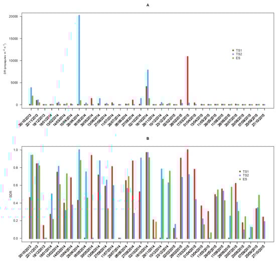
Figure 1.
Time series of the propagule deposition pattern of Cryphonectria parasitica. The average propagule deposition rate (DR) is reported in propagules·m−2·h−1 (panel A), and the corresponding standardized deposition rate (SDR, Panel B) is shown. Deposition rates are displayed for the different study sites (TS1, TS2, and ES) and sampling dates in the period between October 2013 and October 2015.
3.3. Temporal Variables Related to the Propagule Deposition of C. parasitica
Seasonal patterns displayed by the average DR values of Cryphonectria parasitica at TS locations showed two peaks during the spring and fall, with 1695 propagules·m−2·h−1 (179–5318 CI95%) and 1201 propagules·m−2·h−1 (445–2827 CI95%), respectively, while the DR dropped to 189 propagules·m−2·h−1 (80–437 CI95%) in the summertime and 201 propagules·m−2·h−1 (85–419 CI95%) in the wintertime (Figure 2A). Although the mean DR values substantially differed, such differences were not significant since the meteorological season (SM) and calendar month (MS) of samplings resulted in c statistics with p-values over the threshold 0.05 (i.e., c = 3.68 and p = 0.507 for SM; c = 0.291 and p = 0.831 for MS) (Figure 2A). Similar results were obtained from the unbiased recursive partitioning tree models fitted on the SDR, whose values were similar across seasons, ranging from 0.410 (0.233–0.585 CI95%) in the wintertime to 0.493 (0.328–0.671 CI95%) in the fall, with non-significant c values for both SM (c = 0.604 and p = 0.989) and MS (c = 1.133 and p = 0.492) (Figure 2B). Conversely, when the average SDR values were filtered by applying increasing sequential thresholds, significant effects of the sampling season SM (c = 11.448 and p = 1.89·10−2) on the filtered SDR* were detected for n = 6, corresponding to a background noise threshold t* of 60 propagules·m−2·h−1 (i.e., level of propagule discharge released by C. parasitica regardless of the season). In fact, the average propagule deposition of C. parasitica over the baseline of 60 propagules·m−2·h−1 was significantly higher in the spring and fall (SDR* = 0.838–0.911) than in the summer and winter (SDR* = 0.693–0.759) (p < 0.05) (Figure 2C).
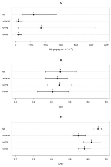
Figure 2.
Seasonal patterns of the propagule deposition of Cryphonectria parasitica. Dots represent the mean rate of propagule deposition (DR) in propagules·m−2·h−1 (panel A), the average standardized deposition rate (SDR, panel B), or the average SDR of C. parasitica over the baseline of 60 propagules·m−2·h−1 (SDR*, panel C) for each season. Whiskers around the dots refer to the 95% confidence intervals. Different letters are used to highlight significant differences (p < 0.05).
Instead, no significant effects of the calendar month (MS) of sampling on SDR* were detected (c = 0.189 and p = 0.887). The cosine regression model showed that the average SDR* followed a seasonally-driven periodic behavior (Figure 3). All parameters of the regression equation were significant, with (t = 36.690 and p < 0.001), (t = 151.150 and p < 0.001), and (t = 59.360 and p < 0.001). The residuals of the model were normally distributed based on the Shapiro–Francia statistics (W = 0.953 and p = 0.193). In comparison to the null model, the cosine regression showed a lower AICc (−40.200 vs. −30.600) and a higher AICcw (0.992 vs. 0.008), thus confirming its adequacy. The cosine regression model run on data from ES was successfully validated since the corresponding OP regression displayed coefficients and comparable to 1 (p = 0.771) and 0 (p = 0.785). The average predicted SDR* values were 0.762 (0.685–0.838 CI95%) and 0.692 (0.628–0.756 CI95%) in the winter and summer, respectively, and 0.840 (0.767–0.913 CI95%) and 0.909 (0.832–0.985 CI95%) in the spring and fall (Figure 3), respectively. These values were consistent with the average SDR* values observed during the same seasons in ES, reaching 0.704 (0.621–0.765) in the winter, 0.727 (0.606–0.924) in the summer, 0.856 (0.757–0.916) in the spring, and 0.889 (0.818–0.929) in the fall.
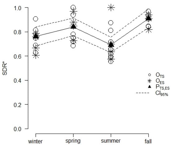
Figure 3.
Results from the cosine regression modelling of the average SDR of Cryphonectria parasitica over the baseline of 60 propagules·m−2·h−1 (SDR*) as a periodic function of the season. Points mark the average SDR* observed during the 4 seasons in TS (OTS) and ES (OES) or the average SDR* values predicted by the model for the TS and ES sites (PTS,ES) with the related 95% confidence intervals (CI95%). Observed SDR* values refer to each sampling whose corresponding DR was larger than 60 propagules·m−2·h−1, while predicted SDR* results are the outcomes of the cosine regression model. Segments are used to link dots related to model predictions, highlighting the periodic seasonal fluctuation of the SDR*.
3.4. Climatic Variables Associated with the Propagule Deposition of C. parasitica
A total of 3 out of 88 climatic variables tested for their association with the standardized deposition rate (SDR) of Cryphonectria parasitica displayed a significant c value (p < 0.05), namely the number of days with precipitations over 1, 2, and 5 mm occurring during the 7 days preceding each sampling (i.e., NDP17, NDP27, and NDP57) (Table 1). Overall, the outcomes of the tree models showed that an increasing number of rainy days during the week was positively correlated with raising SDR values at the end of the week (p < 0.05). In detail, the average SDR in the absence of rainy days providing over 1 mm/day of water was 0.278 (0.167–0.424 CI95%), but if at least one such day occurred, the average SDR jumped up to 0.534 (0.449–0.616 CI95%) (p = 2.67·10−2). The same pattern resulted from the analysis of the number of weekly days with a rain intensity over 2 and 5 mm/day. In those cases, the average SDR significantly increased from 0.296 (0.194–0.423 CI95%) to 0.541 (0.447–0.629 CI95%) (p = 2.56·10−2) and from 0.313 (0.219–0.423 CI95%) to 0.578 (0.481–0.664 CI95%) (p = 1.22·10−2), respectively. Conversely, no significant effects (p > 0.05) on the SDR were displayed by the same climatic variables when considered over different timeframes (i.e., NDP1i, NDP2i, and NDP5i with i = 14, 21, and 30, respectively). The SDR was also not significantly correlated (p > 0.05) to other climatic covariates related to precipitations (Psumi, Pmeani, NDP0i, NDP10i, NDP15i, NDP20i, NDP25i, and NDP30i), humidity (RHmeani, RHmaxi, and RHmini), temperatures (GDD0i, GDD5i, Tmeani, Tmaxi, and Tmini), and wind (WSi, WGi, and TCWi) regardless of the considered timeframe (Table 1).

Table 1.
Results from unbiased recursive partitioning tree models testing the association between the standardized spore deposition rate (SDR) of Cryphonectria parasitica and the climatic variables. For each climatic variable and associated timeframe (i in days prior to samplings), the c statistics are reported with corresponding p-values. The * symbol indicates significant c values, namely significant associations between the SDR and the climatic variable (p < 0.05).
The OLSLR modelling of the SDR as a function of NDP17, NDP27, and NDP57 showed a significant (p < 0.05) and positive (m > 0) linear trend relating higher values of the SDR to increasing numbers of weekly rainy days (Figure 4). All models fulfilled the imposed conditions, resulting in significant t-statistics of the m and q coefficients (p < 0.05), a significant F test, a non-significant Shapiro–Francia test for the model residuals, and OP regression coefficients m′ and q′ comparable to 1 (p > 0.05) and 0 (p > 0.05), respectively (Table 2). Based on the values of R2 (ranging from 0.126 to 0.127), Theil’s UII (from 0.527 to 0.533), AICc (from 34.908 to 42.200), and AICcw (from 0.013 to 0.518) the most performant model was that fitted on NDP57, followed by NDP27 and NDP17 (Table 2). All models were successfully validated, as shown by the outcomes of the OP regressions reported in Table 2. Ranking based on the external validation indexes RMSEP (ranging from 0.253 to 0.265) and Theil’s UII (from 0.463 to 0.484) indicated that the best model was based on NDP17, followed by the models fitted on NDP27 and NDP57. The values achieved by climatic variables associated with each sampling are reported in Table S2.
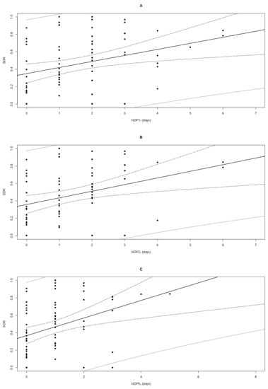
Figure 4.
Linear regressions modelling the propagule deposition pattern of Cryphonectria parasitica to the number of days with precipitations over 1, 2, and 5 mm (NDP17—panel A; NDP27—panel B; and NDP57—panel C, respectively) occurring during a timeframe of 7 days. The graphs show the positive correlation between increasing values of NDP17, NDP27, and NDP57 (on the x-axis) and the raising standardized deposition rate (SDR) of C. parasitica (on the y-axis). The points indicate the observed SDR in sites TS1 and TS2, while the continuous lines represent the equations of the regression models. Confidence and prediction intervals at 95% are shown as dashed and dotted lines, respectively.
Table 2.
Propagule deposition of Cryphonectria parasitica modelled as a function of climatic variables. The table shows the outcomes of the ordinary least squares linear regressions (OLSLR) modelling of the standardized deposition rate (SDR) of C. parasitica based on the number of days with weekly precipitations over 1, 2, and 5 mm (x), namely NDP17, NDP27, and NDP57, respectively. The first row refers to the null model. RT, FT, and SFT are abbreviations for the Ramsey, F, and Shapiro–Francia tests, respectively. The model equation slope (m) and intercept (q) are reported for all models, with their p-values in brackets. The same coefficients are presented for the slope (m′) and intercept (q′) of the regressions between observed and predicted (OP) values of the SDR, but in this case, with expected values m′ = 1 and q′ = 0 under the null hypothesis. The index R2, Theil’s UII, Akaike criteria AICc and AICcw, and the root mean square error of prediction (RMSEP) are also indicated. Statistics showing “e” in the subscript refer to the external validation of the OLSLR model. When appropriate, the p-value is reported in brackets under the related statistics. The symbol (*) indicates significant values (p < 0.05).
3.5. Spatial Patterns of the Propagule Deposition of C. parasitica
Overall, the spatial patterns displayed by the deposition rate (DR) of C. parasitica in the three sites was either random or clustered. In detail, the Bartels test was non-significant in TS1 (Standardized Bartels Statistic SBS = −0.329 and p = 0.742) and ES (SBS = −0.838 and p = 0.402) and significant in TS2 (SBS = −2.532 and p = 0.011), indicating the spatial randomness of the DR in the first two sites and non-randomness in the latter. The Moran’s index confirmed the random spatial pattern in TS1 (I = −0.072 and p = 0.919) and ES (I = 0.094 and p = 0.438), while in TS2 the non-randomness resulting from the Bartels test was detected as positive spatial autocorrelation (i.e., spatial clustering) of the DR values (I = 0.534 and p = 0.007). With the exception of TS1, where the first trap showed a spatial discontinuity (c = 4.378 and p = 0.036), no significant spatial breaks in the DR sequence were detected in TS2 (c = 0.484 and p = 0.486) and ES (c = 0.010 and p = 0.919) (Figure 5).
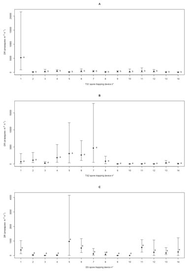
Figure 5.
Patterns of the spatial propagule deposition of Cryphonectria parasitica. For sites TS1 (panel A), TS2 (panel B), and ES (panel C), the mean deposition rate (DR) of the fungal pathogen and the 95% confidence interval are displayed for the different spore traps labelled from 1 to 14 as dots and t-shaped lines, respectively. Different letters are used to highlight significant differences (p < 0.05) among average DRs depending on the spore trap locations along the linear transect.
4. Discussion
Quantifying the propagule deposition of Cryphonectria parasitica and investigating its patterns in relation to temporal and climatic variables may provide key information for the management of chestnut orchards. It should be noted that this pathogen is acknowledged for its detrimental impact on agriculture and forestry and is a protected-zone quarantine pest in the European Union according to the Commission Implementing Regulation 2019/2072.
To quantify the propagule deposition of C. parasitica, we used a solid experimental design that had already proven its reliability in a previous study targeting G. castaneae [27]. Based on reports from Guerin et al. (2001) [29] and Lione et al. (2021) [27], a high variability of propagule loads of C. parasitica was expected, so we sought to achieve an adequate sampling size, temporal and spatial representativeness through an aerobiological assay hinging on a relevant sampling effort. Almost 1300 samples were collected from 42 passive spore trap devices that were exposed for over two years in three sites of the Alpine district of North Western Italy separated by distances ranging from 15 to 94 km.
The assessment of the performance of the qPCR assay showed that primers performed adequately also when combined with SYBR Green dye technology, rather than with the TaqMan probe used in the work of Chandelier et al. (2009) [34]. LOD and LOQ were tested in two matrices to appraise the possible effects exerted by non-target fungal DNA and PCR inhibitors that could be present in spore traps exposed in the field. Even though LOD and LOQ values obtained when C. parasitica DNA was diluted in the environmental matrix were larger than those obtained from dilutions in water, the genomic DNA of C. parasitica could be detected and quantified up to the magnitude of femtograms in both cases. Accordingly, the LOQ obtained from the standard curve of conidia was adequate, corresponding to 7 propagules·m−2·h−1. Therefore, we also showed that the primers designed by Chandelier et al. (2019) [34] could be successfully used on samples that contain less PCR inhibitors compared to bark and wood tissues, which are notoriously recalcitrant matrices [62]. It should be noted that this qPCR assay was not designed to differentiate sexual and asexual propagules. Nonetheless, this has been reported as a minor issue for those fugal pathogens whose sexual spores and conidia are both infectious, as in the case of C. parasitica [27,63].
While a previous study had quantified the propagule loads of C. parasitica [29] and documented its seasonal relation with the peculiar climatic patterns of the Atlantic coast of Western France [64], no information was available for other parts of Europe, including the Alpine region of North Western Italy. It is worth noting that the European Atlantic regions and the Alpine district display distinct climate conditions [65], as well as that sizeable variations of the temporal propagule deposition patterns of the same fungal species may occur among different geographic regions. For instance, this phenomenon was recently documented for the fungal pathogen of chestnut G. castaneae. In fact, while rainfalls have been suggested as the main drivers eliciting spore loads of G. castaneae and host infection in the Southern Hemisphere, temperatures and wind seem to play major roles in Europe (see [12,27] and the literature therein). A further reason to investigate the propagule deposition of C. parasitica in a different geographic area is the fact that fungal sporulation can be driven not only by climate and seasonality but also by topography, landscape structure, and other environmental, epidemiological, or stochastic factors [66,67,68]. Hence, the comparison of results gathered from aerobiological assays conducted in different regions may provide a more thorough understanding of the pathogen sporulation patterns, by implicitly accounting for the underlying spatial variability [45,69]. This is of the outmost importance to predict the risk of infection in different geographic areas, since airborne propagules represent the biological stage epidemiologically most relevant. In fact, airborne propagules are responsible of the establishment and spread of plant pathogens in new crops and orchards [70].
The temporal propagule deposition patterns displayed by C. parasitica showed alternating fluctuations of peaks and troughs, with overall values characterized by high variability at the sampling, seasonal, and site levels, as clearly indicated by the magnitude of the 95% bootstrap confidence intervals of the average DR and SDR. It is worth noting that the mean values of both deposition rates were distributed according to a visible seasonal pattern, with approximately equivalent peaks in the spring and fall counterbalanced by substantial winter and summer drops, though this pattern was not significant. However, once the deposition rate of C. parasitica was filtered by retaining only those values over a given threshold, a significant effect of seasonality could be detected by the tree models. This result may be relevant under many perspectives. In fact, the raw and seasonal deposition rates indicate that C. parasitica could release infectious inoculum all over the year. This continuous propagule discharge may have represented a sort of background noise masking the effects of seasonality on the temporal deposition patterns. In fact, the effect of seasonality was detected as significant only once the iterative algorithm based on sequential threshold filtering was run. The algorithm outcomes suggest that the level of background noise can be estimated at approximately 60 propagules·m−2·h−1. Hence, due to the presence of this background noise, the risk of infection for chestnuts growing in orchards of the Alpine region of North Western Italy is virtually not negligible regardless of the season. However, deposition rates over 60 propagules·m−2·h−1, which are likely related to a higher risk of infection [71], display a significant seasonality with fall and spring peaks, followed by winter and summer drops. The significant role of seasonality as a driver of the propagule deposition of C. parasitica was confirmed not only by the tree models but also by the cosine regression that demonstrated the periodic pattern of deposition rates over 60 propagules·m−2·h−1. The internal assessment of the trigonometric model and its external validation highlighted the robustness of the relation between seasonality and propagule loads of C. parasitica. Although the two peaks detected in the spring and fall were almost equal, they are unlikely to be comparable in terms of risk of infection. In fact, some studies [72,73] have shown that the period of highest receptivity of chestnut to C. parasitica occurs during springtime in Europe, so propagules released in that period are more likely to cause new infections than those discharged during the fall peak.
Not surprisingly, the seasonal pattern observed in the Alpine district differed from that reported by some studies conducted in other geographic areas. For instance, Guerin et al. (2001) [29] showed that in Western France C. parasitica released spores between March and October, with a single peak during the spring. The humped shape of the spore abundance curve presented in that study is only partially consistent with our findings, which highlight a bimodal pattern due to the presence of a second peak in the fall. However, studies conducted in the US confirm that C. parasitica can release infectious propagules all over the year, with a peak occurring in late summer or fall [74,75]. These lines of evidence suggest that spore dispersal maxima are dependent on local geographical and climactic features.
Since the discrepancies among seasonal deposition patterns observed across different geographic regions might have been due to climatic factors, we carried out a comprehensive climatic analysis by accounting for 88 variables related to temperatures, rainfalls, humidity, and wind. The tree models showed that only some variables related to rainfalls were significantly correlated with the temporal propagule deposition patterns of C. parasitica, instead temperatures, humidity, and wind were not significant. Interestingly, we observed that an increasing number of days with precipitations over 1, 2, and 5 mm occurring during the week before samplings was associated with a significant raise of propagule loads of the pathogen. Based on the overall outcomes of the tree models, the expected propagule loads of C. parasitica during a week without precipitations were almost a half of those observed if at least one day with over 1–5 mm of rain had occurred. Linear regressions added further information by unravelling the relation between the increment of rainy days and the corresponding raise of the standardized propagule deposition rate. Based on the values attained by the slope (m) of the regression equations, each additional rainy day increases the expected amount of airborne propagules released by C. parasitica by 7–10%. These models provide new practical tools to support risk assessment by requiring, as input, variables whose measurement is relatively easy to conduct and equally easy to retrieve from local networks of agro-meteorological stations [27,30,37]. From this perspective, the application of the above-described models might help in planning the activities for the management of chestnut orchards. For instance, when operations implying wounds on stem and branches are foreseen, they could be profitably delayed or anticipated (if feasible) when days with over 1–5 mm of accumulated rainfall are absent or likely to be absent during the preceding 7 days. In fact, when the release of massive propagule loads by C. parasitica is less likely, the risk of host infection through fresh wounds should be lower as well. Interestingly, the linear models agreed with the results of the seasonality analyses, which showed the existence of a background propagule discharge of C. parasitica regardless of the season. In fact, the linear equations displayed positive intercepts (q) significantly different from 0, thus suggesting that a baseline release of propagules was present regardless of the number of rainy days occurring during the week. Despite the linear regressions being significant and successfully validated, they should be used with caution, since the low values of the R2 indicate a large variability of the outcome response variable. Although fully comparable in terms of performance, the most consistent model was that based on the 2 mm threshold, whose ranking was the same when considering both internal and external validation metrics. It is noteworthy that when the threshold was increased to 10–30 mm or was lower than 1 mm, the corresponding number of rainy days was not correlated to the temporal propagule deposition pattern of the pathogen. Overall, this finding seems to imply that the daily water input able to boost the sporulation of C. parasitica ranges from 1 to 10 mm. It could be argued that lower precipitations were not effective in supporting the mechanical processes underlying the liberation of propagules, probably because the level of humidity needed to release the sexual spores could not be reached or the mass of rain drops was not adequate to prompt the splash dispersal of conidia [63,76]. Conversely, more intense rainfalls could have intercepted the airborne propagules, bringing them to the soil and hence reducing their abundance [76]. Interestingly, Prospero and Rigling (2013) [63] reported that a rainfall event of 4.5 mm could induce an abundant sporulation of C. parasitica, and that value is fully consistent with the thresholds of daily precipitation identified as significant by our models (i.e., 1–5 mm). Although our study was not conceived to investigate the mechanical effects of the raindrops on the propagule loads of C. parasitica, the fact that the temporal propagule deposition was correlated to the number of rainy days, rather than to the overall amount of water input, seems to support the above-mentioned hypothesis. In fact, the same amount of rain accumulated during the week might result from either a few intense events or from more frequent but milder precipitations. Similarly, relative humidity may be high regardless of the intensity of the rainfall triggering the moisture levels, thus explaining the lack of correlation between this climatic variable and the propagule deposition rates of C. parasitica. The positive correlation between the deposition rates of C. parasitica and rainfall events has also been confirmed by previous reports [29,75,77]. It is worth noting that the spring and fall are the seasons where rainfalls are more frequent in the Alpine region, while summer is usually dryer. These climatic conditions could explain why we detected a bimodal propagule deposition pattern with peaks during spring and fall.
The association between temperatures and chestnut blight was investigated in previous studies [72]. For instance, it was reported that the main driver boosting the spread of C. parasitica in North America was air temperature and that warming conditions were more favorable to the pathogen [78]. Accordingly, positive correlations between the abundance of propagules released by C. parasitica and maximum, minimum, and mean temperatures were detected in France, with the highest correlation coefficients displayed by the maximum temperature [29]. Conversely, the results from our study showed that variables related to temperatures (including growing degree days) were not significantly related to the temporal propagule deposition patterns of C. parasitica. Though we believe that our experiment was adequate to appraise the potential role of temperature on the propagule deposition rates of C. parasitica, since such association was detected in a similar study targeting G. castaneae in the same sites and during the same period [27], an overall effect of temperature cannot be completely ruled out. In fact, climatologic investigations [79] have provided a solid line of evidence demonstrating that the temperatures of the Alpine district of North Western Italy have substantially raised in recent years. In particular, air temperatures have been over those of the reference period (1971–2000), displaying an increase of approximately +1 °C in 50 years for the average temperature and +2 °C for the maximum temperature [79]. Assuming that C. parasitica might be favored by warming temperatures, an overall increase of the latter due to climate change could result in an expansion of the sporulation period that could even last for the whole year. This hypothesis is consistent with our findings showing that C. parasitica can release propagules all over the year, with a background deposition estimated at 60 propagules·m−2·h−1. In addition, the negative trend of the snow accumulation in the Alpine district of North Western Italy (see [79] and literature therein) might have played a role. Due to climate change, the snow layer that should cover soil, wood residuals, living trees, and branches is often absent in the wintertime or lasts for a reduced period. This implies that the fruiting bodies of C. parasitica are not covered as much as they would be if snowfalls were more abundant. This would explain why C. parasitica is able to discharge propagule loads also during the winter. It is worth mentioning that an important substrate for the production of airborne inoculum of C. parasitica is represented by all kind of debris and dead wood residuals of chestnut that can be present at the ground level [21] and that could be fully covered by the snow layer in the wintertime. While dead wood may not be particularly abundant in chestnut orchards, coppices hosting relevant amount of necromass are often grown in their close proximity as part of agroforest systems [15]. Hence, climate change might provide some clues to understand why C. parasitica could produce airborne inoculum according to the patterns that we observed and, especially, why we detected a stable background deposition rate in the Alpine district of North Western Italy. Nonetheless, these should be regarded as mere hypotheses, since no data about the propagule loads of C. parasitica are available to enable comparisons between the current situation and that occurring prior to temperature rises and snowfall shrinkages in this geographic district.
Although wind may be a key factor for the successful release and dissemination of airborne propagules of fungi [27,66], our analyses showed that it did not exert a significant effect on the temporal spore deposition patterns of C. parasitica. This result might be explained considering that C. parasitica can reproduce both sexually and asexually [63]. While sexual ascospores are mainly windborne and can reach remarkable distances in the order of some hundred meters, the asexual conidia of C. parasitica are mainly splash-dispersed by raindrops within a short range from the source in the order of magnitude of a few meters [63]. If asexual reproduction was prevalent, the effect of wind on the propagule deposition would unlikely be significant. However, since our experimental design could not differentiate between loads of spores and conidia and since no information about the populations’ structure of C. parasitica was available for our study sites, we cannot confirm or reject this hypothesis. In addition, other spreading pathways of the propagules of C. parasitica other than wind and rainfalls have been documented, including insects and other animals (see [63] and literature therein), but the spore trapping method presented in our study was not suitable to intercept such vectors. More importantly, the vitality of spores and conidia may differ based on environmental conditions (e.g., conidia deposited at the soil level may remain viable for long times, while spores are often short-living) [63], and further studies may be needed to appraise the overall risk of infection deriving from the combination of propagule abundance and vitality.
In our study, the spatial pattern of the propagule deposition of C. parasitica was investigated for the first time at the within-site scale. Our results showed that the spatial distribution of the propagule deposition was either random or clustered, depending on the site. In other terms, when spatial randomization occurred, high and low average values of propagule deposition were distributed without a significant trend along the linear transect [69]. Conversely, when spatial clustering was detected, spore traps with high and low values of propagule deposition tended to be surrounded by traps displaying similar values [69]. Based on these results, it seems likely that both sexual spores and conidia landed onto the spore traps. In fact, as suggested by Lione et al. (2021) [27], clustering could be a clue suggesting the prevailing asexual reproduction and the presence of propagule sources in close proximity to the spore traps devices, while randomization might be more consistent with the sexual reproduction pattern. Nonetheless, even where randomization occurred, the presence of a spatial discontinuity may suggest that conidial loads were also discharged. As previously remarked, our experiment was not aimed at investigating the population structure of C. parasitica, but the spatial pattern can provide a useful proxy to formulate the hypothesis that both sexual and asexual reproduction occurred [26,27]. This conclusion seems to be supported by studies reporting the presence of both mating types of C. parasitica in Italy, thus allowing the pathogen to reproduce sexually other than asexually [63,80,81].
The results from our study are only partially comparable to those provided by other aerobiological experiments, not only because they refer to different geographic areas but also because the spore trapping and quantification methods (including the unit of measurement) were different. However, our data can be fully contrasted with those obtained for G. castaneae, whose propagule loads were investigated with the same methods, in the same sites, and during the same periods [27]. Remarkably, C. parasitica produced an up-to 5-fold higher average abundance of airborne propagules than G. castaneae. In addition, the upper levels of the confidence intervals associated with the above-mentioned averages were up to 10-fold higher in the case of C. parasitica, indicating that peaks of propagule discharge were even more pronounced. Considering that G. castaneae is an emerging pathogen that has been reported also as a canker agent on chestnut (see in [12]), this observation suggests that the potential risk of infection associated with C. parasitica is comparatively higher, at least in the Alpine district of North Western Italy. Hence, C. parasitica can be scored as one of the major, if not the major threat to chestnut in that geographic area. In addition, since global climate change and extreme events, such as hailstorms, have been reported as drivers of the resurgence of chestnut blight [15], the risk of damage and losses for chestnut growers is likely destined to increase in the near future. As a final remark, since the size of wounds on chestnut bark is positively associated to the risk of infection by C. parasitica [15], management operations in orchards should be conducted with caution. Preventing injuries to chestnut is likely the most simple and recommendable strategy to hinder the penetration of infectious inoculum, especially during the spring and fall seasons, and after the occurrence of rainy days with precipitations between 1 and 10 mm during the week.
5. Conclusions
Overall, the results of this study indicate that in the Alpine district of North Western Italy C. parasitica can release propagules all year round, with seasonal massive peaks in spring and fall. These peaks are positively correlated to the number of rainy days during the week with precipitations ranging from 1 to 10 mm/day. Furthermore, the spatial pattern of propagule deposition is consistent with the presence of both sexual and asexual reproduction. Since C. parasitica infects chestnuts via propagules (i.e., sexual spores and asexual conidia) penetrating through fresh wounds, the risk of infection can be appraised by predicting the likelihood of high propagule loads based on seasonality and climate. The results presented in this study have clear implications for the management of orchards affected by the disease.
Supplementary Materials
The following supporting information can be downloaded at: https://www.mdpi.com/article/10.3390/agriculture12050644/s1. Figure S1. Melting curves of the specificity assay. Figure S2. Standard curves of the sensitivity assay. Table S1. Fungal isolates used to assess the specificity of the qPCR assay for Cryphonectria parasitica. Table S2. Propagule deposition rate of Cryphonectria parasitica and climatic variables.
Author Contributions
Conceptualization, G.L. and P.G.; methodology, G.L., F.B., L.G. and P.G.; formal analysis, G.L.; investigation, G.L. and F.B.; resources, P.G.; data curation, G.L.; writing—original draft preparation, G.L. and F.B.; writing—review and editing, P.G.; visualization, G.L.; supervision, P.G.; project administration, P.G.; funding acquisition, P.G. All authors have read and agreed to the published version of the manuscript.
Funding
This research was co-funded by Regione Piemonte through the F.E.A.S.R. 2014/2020, Projects #castagnopiemonte and 3C (Progetti pilota per la Cooperazione ed il miglioramento della Competitività della Castanicoltura regionale), through the activity of the Chestnut R&D Center, and by the European Commission through the programme INTERREG V-A Italy-Switzerland 2014/2020, Project MONGEFITOFOR id 540693 (linee guida per il MOnitoraggio e la Gestione delle Emergenze FITOsanitarie nelle FOReste delle Alpi centro-occidentali).
Institutional Review Board Statement
Not applicable.
Informed Consent Statement
Not applicable.
Data Availability Statement
All data relevant to this manuscript are provided as Supplementary Material for online publication.
Acknowledgments
The authors wish to thank the owners of chestnut orchards in San Giorio di Susa, Peveragno, and Gaiola for the in-field support, as well as Fabiano Sillo and Riccardo Dipoppa for the laboratory assistance in the processing of spore traps.
Conflicts of Interest
The authors declare no conflict of interest. The funders had no role in the design of the study; in the collection, analyses, or interpretation of data; in the writing of the manuscript, or in the decision to publish the results.
References
- Bounous, G.; Torello Marinoni, D. Chestnut: Botany, horticulture, and utilization. Hortic. Rev. 2005, 31, 291–347. [Google Scholar] [CrossRef]
- Bounous, G.; Beccaro, G. History: Growing and using the chestnut in the world from past to present. In The Chestnut Handbook—Crop and Forest Management; Beccaro, G., Alma, A., Bounous, G., Gomes-Laranjo, J., Eds.; CRC Press: Boca Raton, FL, USA, 2020; pp. 1–4. [Google Scholar]
- Conedera, M.; Manetti, M.C.; Giudici, F.; Amorini, E. Distribution and economic potential of the Sweet chestnut (Castanea sativa Mill.) in Europe. Ecol. Mediterr. 2004, 30, 179–193. [Google Scholar] [CrossRef]
- Gobbin, D.; Hohl, L.; Conza, L.; Jermini, M.; Gessler, C.; Conedera, M. Microsatellite-based characterization of the Castanea sativa cultivar heritage of southern Switzerland. Genome 2007, 50, 1089–1103. [Google Scholar] [CrossRef] [PubMed] [Green Version]
- De Vasconcelos, M.C.; Bennett, R.N.; Rosa, E.A.; Ferreira-Cardoso, J.V. Composition of European chestnut (Castanea sativa Mill.) and association with health effects: Fresh and processed products. J. Sci. Food Agric. 2010, 90, 1578–1589. [Google Scholar] [CrossRef] [PubMed]
- Piccolo, E.L.; Landi, M.; Ceccanti, C.; Mininni, A.N.; Marchetti, L.; Massai, R.; Guidi, L.; Remorini, D. Nutritional and nutraceutical properties of raw and traditionally obtained flour from chestnut fruit grown in Tuscany. Eur. Food Res. Technol. 2020, 246, 1867–1876. [Google Scholar] [CrossRef]
- De Biaggi, M.; Beccaro, G.; Casey, J.; Riqué, P.H.; Conedera, M.; Gomes-Laranjo, J.; Fulbright, D.W.; Nishio, S.; Serdar, U.; Zou, F.; et al. Distribution, Marketing, and Trade. In The Chestnut Handbook—Crop and Forest Management; Beccaro, G., Alma, A., Bounous, G., Gomes-Laranjo, J., Eds.; CRC Press: Boca Raton, FL, USA, 2020; pp. 35–52. [Google Scholar]
- Beccaro, G.L.; Donno, D.; Lione, G.G.; De Biaggi, M.; Gamba, G.; Rapalino, S.; Riondato, I.; Gonthier, P.; Mellano, M.G. Castanea spp. agrobiodiversity conservation: Genotype influence on chemical and sensorial traits of cultivars grown on the same clonal rootstock. Foods 2020, 9, 1062. [Google Scholar] [CrossRef]
- Anagnostakis, S.L. Chestnut breeding in the United States for disease and insect resistance. Plant. Dis. 2012, 96, 1392–1403. [Google Scholar] [CrossRef]
- Mellano, M.G.; Beccaro, G.L.; Donno, D.; Marinoni, D.T.; Boccacci, P.; Canterino, S.; Cerutti, A.K.; Bounous, G. Castanea spp. biodiversity conservation: Collection and characterization of the genetic diversity of an endangered species. Genet. Resour. Crop. Evol. 2012, 59, 1727–1741. [Google Scholar] [CrossRef]
- Beccaro, G.L.; Alma, A.; Gonthier, P.; Mellano, M.G.; Ferracini, C.; Giordano, L.; Lione, G.; Donno, D.; Boni, I.; Ebone, A.; et al. Chestnut R&D Centre, Piemonte (Italy): 10 years of activity. Acta Hortic. 2018, 1220, 133–140. [Google Scholar] [CrossRef]
- Lione, G.; Danti, R.; Fernandez-Conradi, P.; Ferreira-Cardoso, J.V.; Lefort, F.; Marques, G.; Meyer, J.B.; Prospero, S.; Radócz, L.; Robin, C.; et al. The emerging pathogen of chestnut Gnomoniopsis castaneae: The challenge posed by a versatile fungus. Eur. J. Plant Pathol. 2019, 153, 671–685. [Google Scholar] [CrossRef]
- Gonthier, P.; Robin, C. Diseases. In The Chestnut Handbook—Crop and Forest Management; Beccaro, G., Alma, A., Bounous, G., Gomes-Laranjo, J., Eds.; CRC Press: Boca Raton, FL, USA, 2020; pp. 297–315. [Google Scholar]
- Rigling, D.; Prospero, S. Cryphonectria parasitica, the causal agent of chestnut blight: Invasion history, population biology and disease control. Mol. Plant Pathol. 2018, 19, 7–20. [Google Scholar] [CrossRef] [PubMed] [Green Version]
- Lione, G.; Giordano, L.; Turina, M.; Gonthier, P. Hail-induced infections of the chestnut blight pathogen Cryphonectria parasitica depend on wound size and may lead to severe diebacks. Phytopathology 2020, 110, 1280–1293. [Google Scholar] [CrossRef] [PubMed]
- Milgroom, M.G.; Cortesi, P. Analysis of population structure of the chestnut blight fungus based on vegetative incompatibility genotypes. Proc. Natl. Acad. Sci. USA 1999, 96, 10518–10523. [Google Scholar] [CrossRef] [PubMed] [Green Version]
- Robin, C.; Anziani, C.; Cortesi, P. Relationship between biological control, incidence of hypovirulence, and diversity of vegetative compatibility types of Cryphonectria parasitica in France. Phytopathology 2000, 90, 730–737. [Google Scholar] [CrossRef] [PubMed] [Green Version]
- Double, M.L.; Jarosz, A.M.; Fulbright, D.W.; Davelos Baines, A.; MacDonald, W.L. Evaluation of two decades of Cryphonectria parasitica hypovirus introduction in an American chestnut stand in Wisconsin. Phytopathology 2018, 108, 702–710. [Google Scholar] [CrossRef] [Green Version]
- Garbelotto, M.; Frigimelica, G.; Mutto-Accordi, S. Vegetative compatibility and conversion to hypovirulence among isolates of Cryphonectria parasitica from Northern Italy. Forest Pathol. 1992, 22, 337–348. [Google Scholar] [CrossRef]
- Melzer, M.S.; Dunn, M.; Zhou, T.; Boland, G.J. Assessment of hypovirulent isolates of Cryphonectria parasitica for potential in biological control of chestnut blight. Can. J. Plant Pathol. 1997, 19, 69–77. [Google Scholar] [CrossRef]
- Prospero, S.; Conedera, M.; Heiniger, U.; Rigling, D. Saprophytic activity and sporulation of Cryphonectria parasitica on dead chestnut wood in forests with naturally established hypovirulence. Phytopathology 2006, 96, 1337–1344. [Google Scholar] [CrossRef] [Green Version]
- Beccaro, G.; Bounous, G.; Cuenca, B.; Bounous, M.; Warmund, M.; Xiong, H.; Zhang, L.; Zou, F.; Serdar, U.; Akyuz, B.; et al. Nursery Techniques. In The Chestnut Handbook—Crop and Forest Management; Beccaro, G., Alma, A., Bounous, G., Gomes-Laranjo, J., Eds.; CRC Press: Boca Raton, FL, USA, 2020; pp. 119–154. [Google Scholar]
- Beccaro, G.; Bounous, G.; Gomes-Laranjo, J.; Warmund, M.; Casey, J. Orchard management. In The Chestnut Handbook—Crop and Forest Management; Beccaro, G., Alma, A., Bounous, G., Gomes-Laranjo, J., Eds.; CRC Press: Boca Raton, FL, USA, 2020; pp. 155–182. [Google Scholar]
- Gonthier, P.; Garbelotto, M.; Nicolotti, G. Seasonal patterns of spore deposition of Heterobasidion species in four forests of the western Alps. Phytopathology 2005, 95, 759–767. [Google Scholar] [CrossRef] [Green Version]
- Simberloff, D. The role of propagule pressure in biological invasions. Annu. Rev. Ecol. Evol. Syst. 2009, 40, 81–102. [Google Scholar] [CrossRef]
- Lione, G.; Gonthier, P. A permutation-randomization approach to test the spatial distribution of plant diseases. Phytopathology 2016, 106, 19–28. [Google Scholar] [CrossRef] [PubMed] [Green Version]
- Lione, G.; Giordano, L.; Sillo, F.; Brescia, F.; Gonthier, P. Temporal and spatial propagule deposition patterns of the emerging fungal pathogen of chestnut Gnomoniopsis castaneae in orchards of north-western Italy. Plant Pathol. 2021, 70, 2016–2033. [Google Scholar] [CrossRef]
- Levetin, E. Aerobiology of agricultural pathogens. In Manual of Environmental Microbiology, 4th ed.; Yates, M.V., Nakatsu, C.H., Miller, R.V., Pillai, S.D., Eds.; ASM Press: Washington, DC, USA, 2016. [Google Scholar] [CrossRef]
- Guerin, L.; Froidefond, G.; Xu, X.M. Seasonal patterns of dispersal of ascospores of Cryphonectria parasitica (chestnut blight). Plant Pathol. 2001, 50, 717–724. [Google Scholar] [CrossRef]
- Lione, G.; Giordano, L.; Sillo, F.; Gonthier, P. Testing and modelling the effects of climate on the incidence of the emergent nut rot agent of chestnut Gnomoniopsis castanea. Plant Pathol. 2015, 64, 852–863. [Google Scholar] [CrossRef]
- Nosenzo, A. Determinazione degli assortimenti ritraibili dai boschi cedui di castagno: L’Esempio della bassa Valle di Susa (Torino). Forest 2007, 4, 118–125. [Google Scholar] [CrossRef]
- Garbelotto, M.; Smith, T.; Schweigkofler, W. Variation in rates of spore deposition of Fusarium circinatum, the causal agent of pine pitch canker, over a 12-month-period at two locations in Northern California. Phytopathology 2008, 98, 137–143. [Google Scholar] [CrossRef] [PubMed] [Green Version]
- Grosdidier, M.; Aguayo, J.; Marçais, B.; Ioos, R. Detection of plant pathogens using Real-Time PCR: How reliable are late Ct values? Plant Pathol. 2017, 66, 359–367. [Google Scholar] [CrossRef]
- Chandelier, A.; Massot, M.; Fabreguettes, O.; Gischer, F.; Teng, F.; Robin, C. Early detection of Cryphonectria parasitica by Real-Time PCR. Eur. J. Plant Pathol. 2019, 153, 29–46. [Google Scholar] [CrossRef]
- Desimoni, E.; Brunetti, B. About estimating the limit of detection by the signal to noise approach. Pharm. Anal. Acta 2015, 6, 1–4. [Google Scholar] [CrossRef]
- White, T.J.; Bruns, T.; Lee, S.; Taylor, J. Amplification and direct sequencing of fungal ribosomal RNA genes for phylogenetics. In PCR Protocols. A Guide to Methods and Applications; Innis, M.A., Gelfand, D.H., Sninsky, J.J., Eds.; Academic Press: San Diego, CA, USA, 1990; pp. 315–322. [Google Scholar]
- ARPA Piemonte. Banca Dati Meteorologica e Idrologica. 2020. Available online: http://www.arpa.piemonte.it (accessed on 15 October 2020).
- Garbelotto, M.; Schmidt, D.; Swain, S.; Hayden, K.; Lione, G. The ecology of infection between a transmissive and a dead-end host provides clues for the treatment of a plant disease. Ecosphere 2017, 8, e01815. [Google Scholar] [CrossRef] [Green Version]
- DiCiccio, T.J.; Efron, B. Bootstrap confidence intervals. Stat. Sci. 1996, 11, 189–228. [Google Scholar] [CrossRef]
- Wickham, H. A layered grammar of graphics. J. Comput. Graph. Stat. 2010, 19, 3–28. [Google Scholar] [CrossRef]
- Hothorn, T.; Hornik, K.; Zeileis, A. Unbiased recursive partitioning: A conditional inference framework. J. Comput. Graph. Stat. 2006, 15, 651–674. [Google Scholar] [CrossRef] [Green Version]
- Hothorn, T.; Zeileis, A. partykit: A modular toolkit for recursive partytioning in R. J. Mach. Learn. Res. 2015, 16, 3905–3909. [Google Scholar]
- Zeileis, A.; Leisch, F.; Hornik, K.; Kleiber, C. strucchange: An R package for testing for structural change in linear regression models. J. Stat. Soft. 2002, 7, 1–38. [Google Scholar] [CrossRef] [Green Version]
- Pewsey, A.; Neuhäuser, M.; Ruxton, G.D. Circular Statistics in R; Oxford University Press: Oxford, UK, 2013. [Google Scholar]
- Crawley, M.J. The R Book, 2nd ed.; John Wiley & Sons: Chichester, UK, 2013. [Google Scholar]
- Royston, P. A pocket-calculator algorithm for the Shapiro-Francia test for non-normality: An application to medicine. Statist. Med. 1993, 12, 181–184. [Google Scholar] [CrossRef] [PubMed]
- Wagenmakers, E.J.; Farrell, S. AIC model selection using Akaike weights. Bull. Psychon. Soc. 2004, 11, 192–196. [Google Scholar] [CrossRef] [PubMed]
- Ramsey, J.B. Tests for specification errors in classical linear least squares regression analysis. J. R. Stat. Soc. Ser. B Stat. Methodol. 1969, 31, 350–371. [Google Scholar] [CrossRef]
- Piñeiro, G.; Perelman, S.; Guerschman, J.P.; Paruelo, J.M. How to evaluate models: Observed vs. predicted or predicted vs. observed? Ecol. Modell. 2008, 216, 316–322. [Google Scholar] [CrossRef]
- Bliemel, F. Theil’s forecast accuracy coefficient: A clarification. J. Mark. Res. 1973, 10, 444–446. [Google Scholar] [CrossRef]
- Anselin, L. Local indicators of spatial association—LISA. Geogr. Anal. 1995, 27, 93–115. [Google Scholar] [CrossRef]
- Hui, W.; Gel, Y.R.; Gastwirth, J.L. Lawstat: An R package for law, public policy and biostatistics. J. Stat. Soft. 2008, 28, 1–26. [Google Scholar] [CrossRef] [Green Version]
- R Core Team. R: A Language and Environment for Statistical Computing; R Foundation for Statistical Computing: Vienna, Austria, 2019; Available online: https://www.R-project.org/ (accessed on 27 October 2019).
- Efron, B.; Tibshirani, R.J. An Introduction to the Bootstrap; Chapman & Hall/CRC: Boca Raton, FL, USA, 1994. [Google Scholar]
- Signorell, A.; Aho, K.; Alfons, A.; Anderegg, N.; Aragon, T.; Arppe, A. DescTools: Tools for Descriptive Statistics. R Package Version 0.99, 18. 2016. Available online: https://cran.r-project.org/web/packages/DescTools/index.html (accessed on 15 February 2022).
- Greenwell, B.M.; Kabban, C.M. Investr: An R package for inverse estimation. R J. 2014, 6, 90–100. [Google Scholar] [CrossRef] [Green Version]
- Kalogirou, S. lctools: Local Correlation, Spatial Inequalities, Geographically Weighted Regression and Other Tools. R Package Version 0.2-8. 2020. Available online: https://CRAN.R-project.org/package=lctools (accessed on 15 February 2022).
- Zeileis, A.; Hothorn, T. Diagnostic checking in regression relationships. R News 2002, 2, 7–10. [Google Scholar]
- Hamner, B.; Frasco, M. Metrics: Evaluation Metrics for Machine Learning. R Package Version 0.1.4. 2018. Available online: https://CRAN.R-project.org/package=Metrics (accessed on 15 February 2022).
- Barton, K. MuMIn: Multi-Model Inference. R Package Version 1.43.6. 2019. Available online: https://cran.r-project.org/web/packages/MuMIn/index.html (accessed on 15 February 2022).
- Baddeley, A.; Turner, R. spatstat: An R Package for analyzing spatial point patterns. J. Stat. Soft. 2005, 12, 1–42. [Google Scholar] [CrossRef] [Green Version]
- Langrell, S.R.H. Development of a nested PCR detection procedure for Nectria fuckeliana direct from Norway spruce bark extracts. FEMS Microbiol. Lett. 2005, 242, 185–193. [Google Scholar] [CrossRef] [Green Version]
- Prospero, S.; Rigling, D. Chestnut blight. In Infectious Forest Diseases; Gonthier, P., Nicolotti, P., Eds.; CAB International: Wallingford, UK, 2013; pp. 318–339. [Google Scholar]
- Calvo-Garrido, C.; Teixidó, N.; Roudet, J.; Viñas, I.; Usall, J.; Fermaud, M. Biological control of Botrytis bunch rot in Atlantic climate vineyards with Candida sake CPA-1 and its survival under limiting conditions of temperature and humidity. Biol. Control 2014, 79, 24–35. [Google Scholar] [CrossRef]
- Raible, C.C.; Casty, C.; Luterbacher, J.; Pauling, A.; Esper, J.; Frank, D.C.; Büntgen, U.; Roesch, A.C.; Tschuck, P.; Wild, M.; et al. Climate variability—Observations, reconstructions, and model simulations for the Atlantic-European and Alpine region from 1500-2100 AD. Clim. Chang. 2006, 79, 9–29. [Google Scholar] [CrossRef]
- Li, D.W.; Kendrick, B. A year-round study on functional relationships of airborne fungi with meteorological factors. Int. J. Biometeorol. 1995, 39, 74–80. [Google Scholar] [CrossRef]
- Peay, K.G.; Bruns, T.D. Spore dispersal of basidiomycete fungi at the landscape scale is driven by stochastic and deterministic processes and generates variability in plant–fungal interactions. New Phytol. 2014, 204, 180–191. [Google Scholar] [CrossRef]
- Schiro, G.; Verch, G.; Grimm, V.; Müller, M. Alternaria and Fusarium fungi: Differences in distribution and spore deposition in a topographically heterogeneous wheat field. J. Fungi 2018, 4, 63. [Google Scholar] [CrossRef] [PubMed] [Green Version]
- Mitchell, A. The ESRI Guide to GIS Analysis, Volume 2: Spatial Measurements and Statistics; ESRI Press: Redlands, CA, USA, 2009. [Google Scholar]
- Reaser, J.K.; Meyerson, L.A.; Von Holle, B. Saving camels from straws: How propagule pressure-based prevention policies can reduce the risk of biological invasion. Biol. Invasions 2008, 10, 1085–1098. [Google Scholar] [CrossRef] [Green Version]
- Kenaley, S.C.; Double, M.L.; MacDonald, W.L. Effect of Spore Concentration on the Establishment of Cytoplasmic Hypovirulent (HV), Transgenic HV, and Virulent Isolates of Cryphonectria parasitica, the Chestnut Blight Fungus. In Proceedings of the Fifth International Chestnut Symposium (Acta Horticulturae), 4–8 September 2012; Double, M.L., MacDonald, W.L., Eds.; ISHS: Korbeek-Lo, Belgium, 2014; pp. 165–171. [Google Scholar] [CrossRef]
- Bazzigher, G. Selection of blight-resistant chestnut trees in Switzerland. Eur. J. For. Pathol. 1981, 11, 199–207. [Google Scholar] [CrossRef]
- Guerin, L.; Robin, C. Seasonal effect on infection and development of lesions caused by Cryphonectria parasitica in Castanea sativa. For. Pathol. 2003, 33, 223–235. [Google Scholar] [CrossRef]
- Heald, F.D.; Gardner, M.W.; Studhalter, R.A. Air and wind dissemination of ascospores of chestnut-blight fungus. J. Agric. Res. 1915, 3, 493–526. [Google Scholar]
- Rankin, W.H. Field studies on Endothia canker of chestnut in New York State. Phytopathology 1914, 4, 233–261. [Google Scholar]
- Kendrick, B. The Fifth Kingdom; Focus Publishing: Newburyport, MA, USA, 2017. [Google Scholar]
- Anderson, P.J. Wind dissemination of the chestnut blight organism. Phytopathology 1913, 3, 1–44. [Google Scholar]
- Anagnostakis, S.L.; Aylor, D.E. The effect of temperature on growth of Endothia (Cryphonectria) parasitica in vitro and in vivo. Mycologia 1984, 76, 387–397. [Google Scholar] [CrossRef]
- Bastiancich, L.; Lasagna, M.; Mancini, S.; Falco, M.; De Luca, D.A. Temperature and discharge variations in natural mineral water springs due to climate variability: A case study in the Piedmont Alps (NW Italy). Environ. Geochem. Health 2021. [Google Scholar] [CrossRef]
- Farooq, A.; Sanja, B. Genetic diversity of Cryphonectria parasitica causing chestnut blight in South Tyrol (northern Italy). Eur. J. Plant Pathol. 2022, 162, 621–635. [Google Scholar] [CrossRef]
- Prospero, S.; Rigling, D. Invasion genetics of the chestnut blight fungus Cryphonectria parasitica in Switzerland. Phytopathology 2012, 102, 73–82. [Google Scholar] [CrossRef] [PubMed] [Green Version]
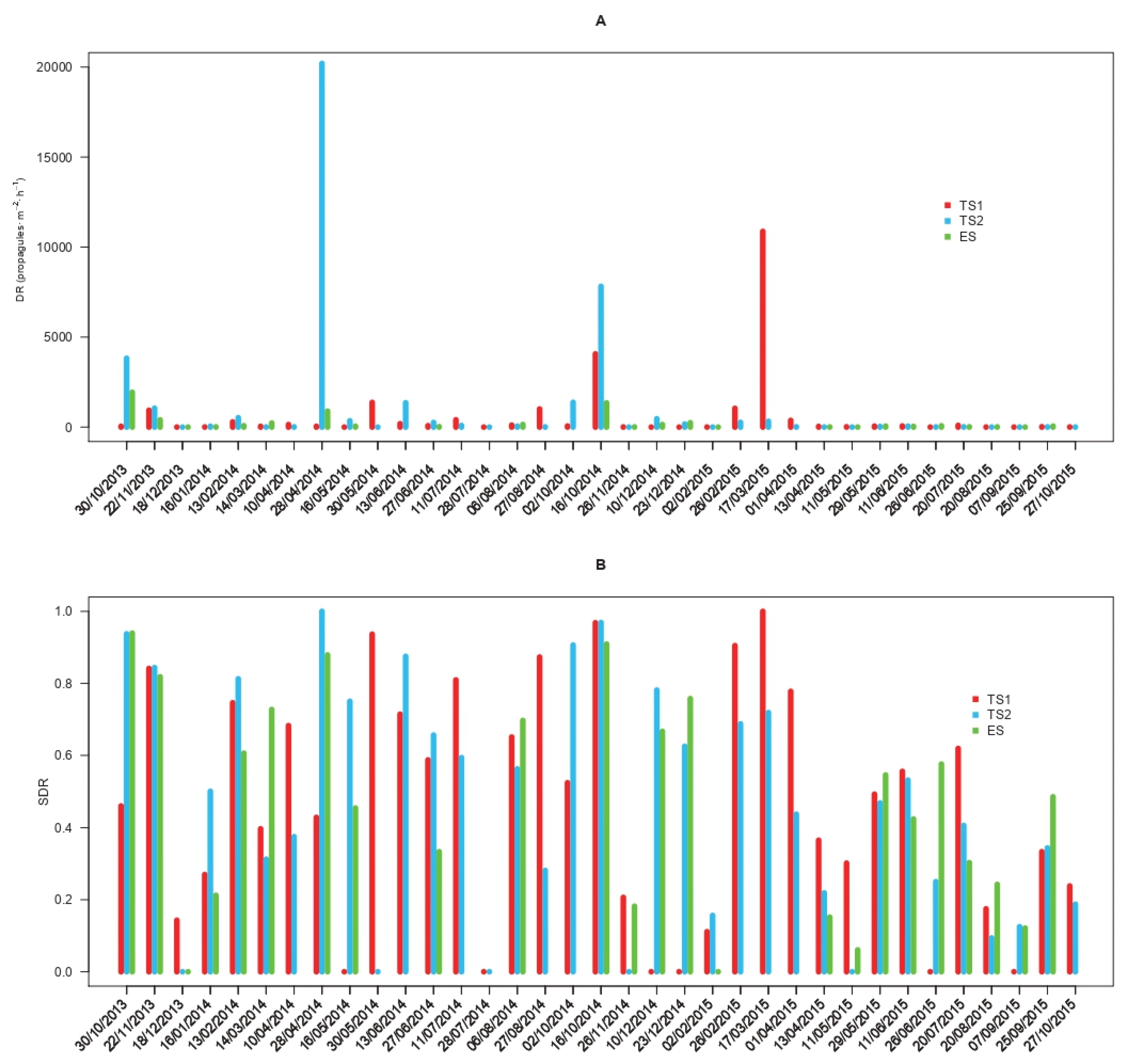
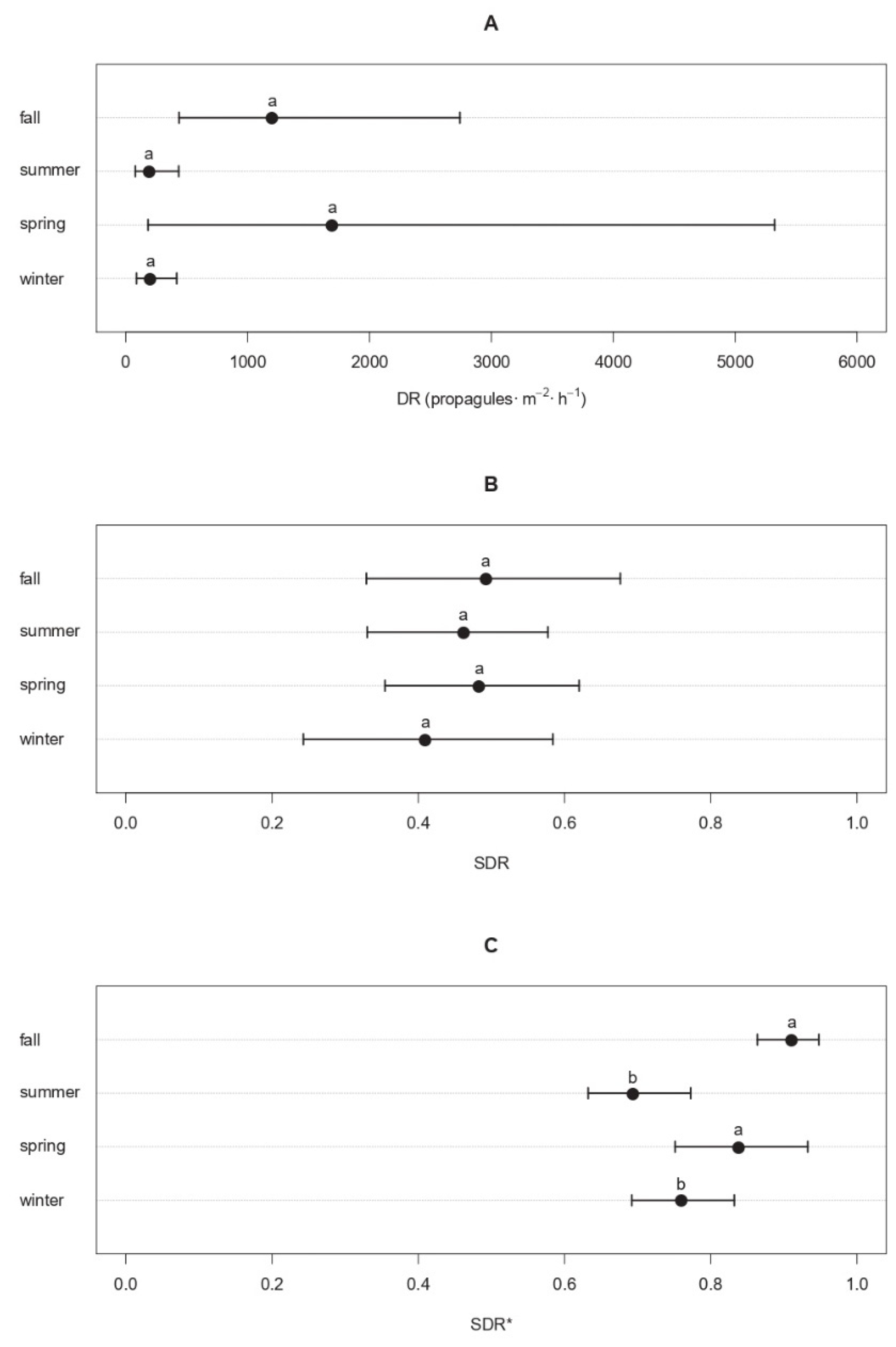
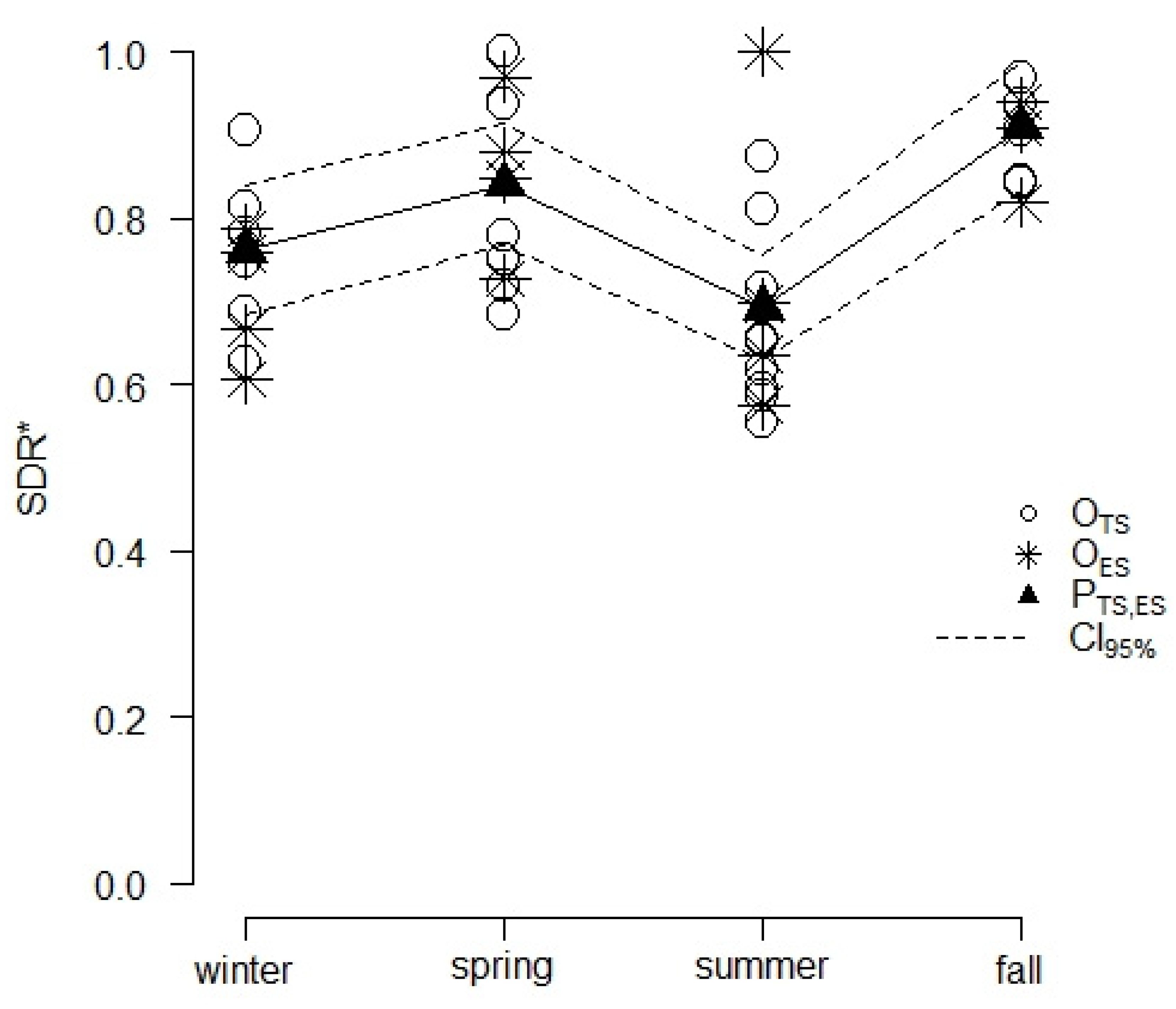
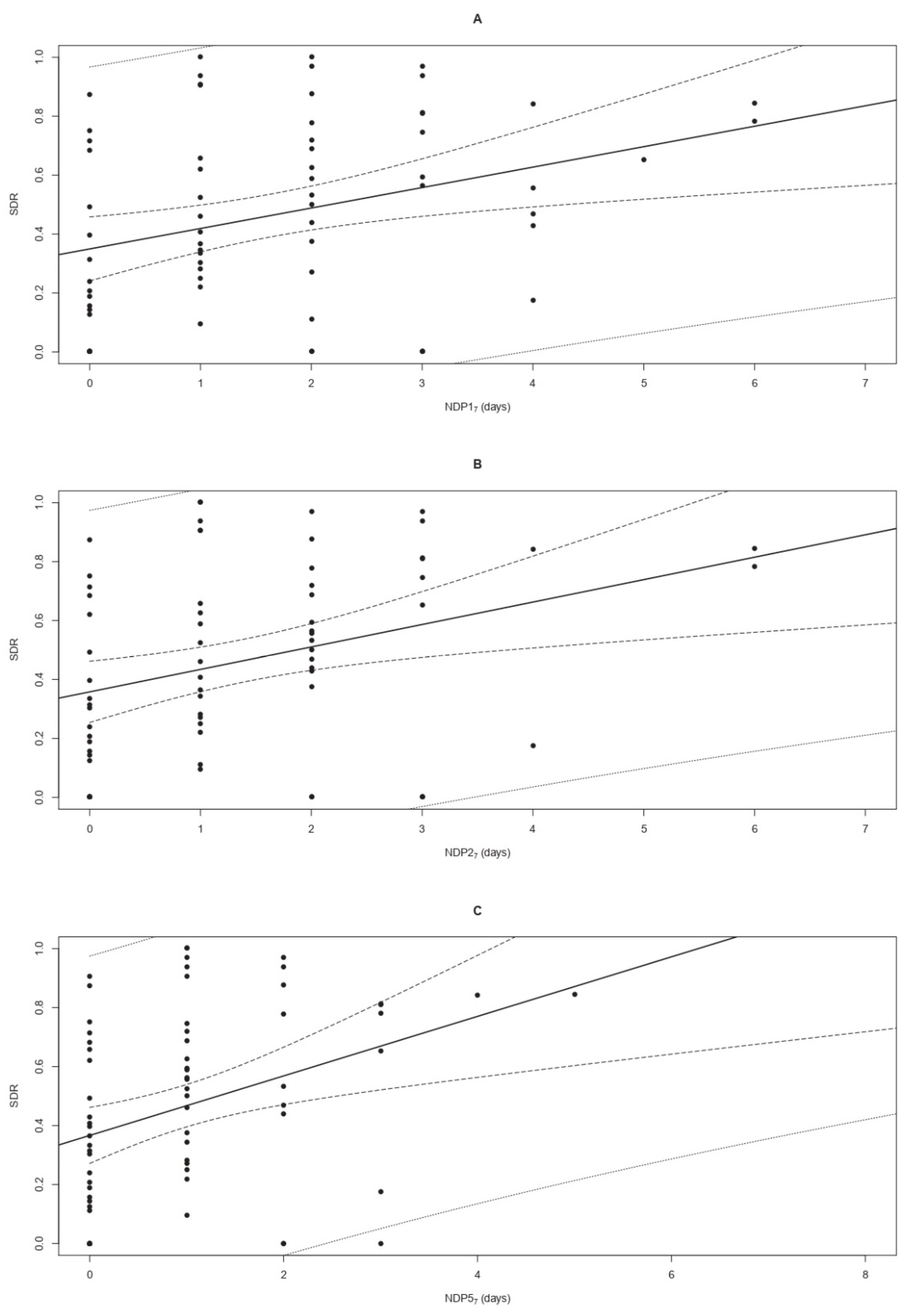
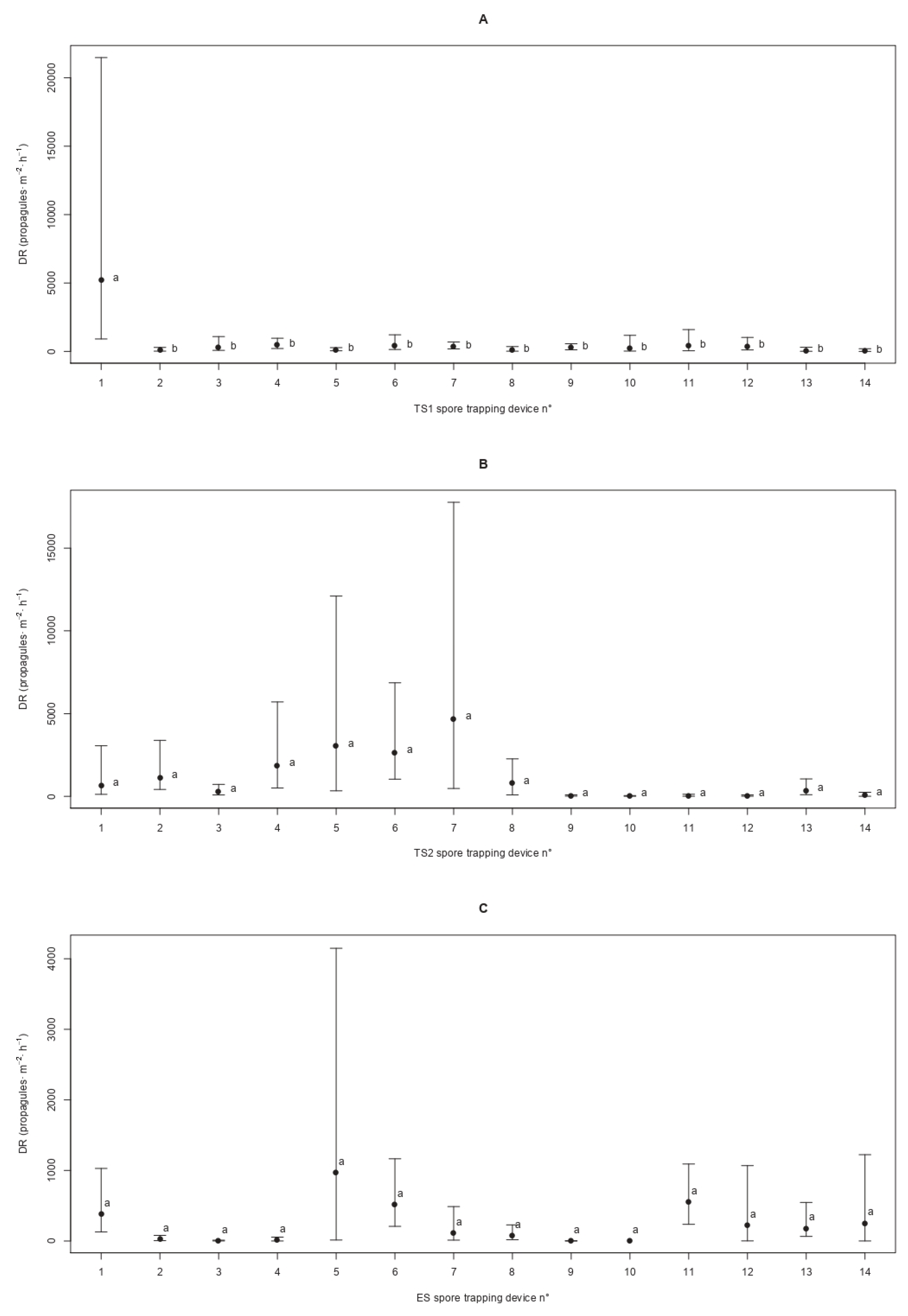
Publisher’s Note: MDPI stays neutral with regard to jurisdictional claims in published maps and institutional affiliations. |
© 2022 by the authors. Licensee MDPI, Basel, Switzerland. This article is an open access article distributed under the terms and conditions of the Creative Commons Attribution (CC BY) license (https://creativecommons.org/licenses/by/4.0/).