Simulating Growth and Evaluating the Regional Adaptability of Cotton Fields with Non-Film Mulching in Xinjiang

Abstract

Planting with non-film mulching is the fundamental means to eliminate the pollution of residual film in cotton fields. However, this planting approach should have regional adaptability. Therefore, the calibrated WOFOST model and an early mature cultivar CRI619 (Gossypium hirsutum Linn) were employed to simulate the cotton growth, and regions were then evaluated for planting in Xinjiang. A field experiment was conducted in 2019–2020 at the experimental irrigation station of Alar City, and the data were used to calibrate and validate the WOFOST model. The field validation results showed that the errors of the WOFOST simulation for emergence, flowering, and maturity were +1 day, +2 days, and +1 day, respectively, with good simulation accuracy of phenological development time. The simulated WLV, WST, WSO, and TAGP agreed well with measured values, with R² = 0.96, 0.97, 0.99, and 0.99, respectively. The RMSE values of simulated versus measured WLV, WST, WSO, and TAGP were 175, 210, 199, and 251 kg ha⁻¹, and showed high accuracy. The simulated soil moisture (SM) agreed with the measured value, with R² = 0.87. The calibration model also showed high SM simulation accuracy, with RMSE = 0.022 (cm³ cm⁻³). Under all treatments, the simulated TAGP and yield agreed well with the measured results, with R² of 0.76 and 0.70, respectively. RMSE of simulated TAGP and yield was 465 and 200 kg ha⁻¹, and showed high accuracy. The percentage RMSE values (ratio of RMSE to the average measured value, NRMSE) of $E{T}_a$ and WUE were 9.8% and 11.7%, indicating extremely high precision (NRMSE < 10%) and high precision (10% < NRMSE ≤ 20%), respectively. The simulated results for phenology length at the regional scales showed that the effective accumulation temperature in counties such as Yingjisha and Luntai was not enough for the phenological maturity of the studied cotton cultivar. The southern area of Xinjiang had a generally higher yield than the northern area but required more irrigation. This research can provide a method for evaluating the adaptability of filmless cultivation techniques for cotton in different counties.

1. Introduction

Cotton is among the essential economic fiber crops and raw materials for the textile industry. China is one of the major cotton lint-producing countries, producing 6,102,800 t, and accounting for about 25% of global cotton production (FAO, 2018). As China’s most significant growth and production region, Xinjiang Uygur Autonomous Region contributes almost 85% of the national cotton fiber production (National Bureau of Statistics of China).

However, the long-term and large-scale use of plastic agricultural film has become a significant factor constraining many aspects of the sustainable development of the Chinese cotton industry. Although other studies have explored many methods in treating mulch film pollution and achieved specific results, the problem is still severe. In 2017, the Cotton Research Institute of the Chinese Academy of Agricultural Sciences successfully bred a new extra-early maturing cotton cultivar (CRI619), suitable for planting without membranes, and conducted a large-scale demonstration application in Shaya County, Aksu Prefecture, that achieved good results. However, whether this cultivar can be demonstrated in other regions of Xinjiang has yet to be proven.

In addition, regional cotton yield assessment in Xinjiang is an indicator for cotton trade and devising planting policies, which have become crucial for ensuring the sustainable development of the cotton industry. However, climate fluctuations in different regions and years can lead to significant variability in yield and water consumption, especially against the background of global warming and climate stress [1,2]. Crop models use mathematical equations to simulate how crop growth and development, photosynthetic production, organ construction, and yield formation are affected by the meteorological environment and agricultural management, and have become an essential means to analyze the climate changes response to crop yields [3].

The development and application of the cotton simulation system began in the United States in the 1960s, and have now expanded to the major cotton production regions worldwide. Mature cotton growth models include GOSSYM [4], COTCO2 [5], OZCOT [6], and CROPGRO-Cotton [7,8]. In addition, some general crop growth models are also used to simulate cotton growth, such as Environmental Policy Integrated Climate (EPIC) [9], World Food Studies (WOFOST) [10], Cropping Systems Simulation Model (CropSyst) [11], and AquaCrop (a crop-water productivity model) [12]. Although there are some differences in the simulated methods, details, and yield components of existing cotton models, the main processes include phenology, light energy interception, carbon (C) assimilation, respiration, organ formation, biomass accumulation and distribution, and stress factor simulation [13]. These models have been used in irrigation management [14,15,16,17,18,19,20,21] and water use efficiency evaluation [22,23,24], assessment of effects of deficit irrigation on cotton growth and yield [25,26,27,28], evaluation of saline water irrigation on cotton growth and yield [29], nitrogen and phosphorus dynamics and fertilization management [14,30,31], fiber quality, embryo oil and protein accumulation simulation [32,33,34], and topping management [35].

These models estimate crop yields by simulating the contribution of meteorology, soil moisture, nutrients, and management to plant growth and development, and have been widely used for simulating climate change impacts on cotton production [36]. The GOSSYM model was employed for estimating US cotton yields and climate stresses from 1979 to 2005, such as water, carbon, and nitrogen stress [37]. The CSM-CROPGRO-Cotton model integrated into DSSAT was used to optimize the cultivars and identify optimum planting dates for optimum cotton growth at all key phenological development stages by utilizing optimal weather conditions [38]. APSIM, AquaCrop, and CROPGRO-Cotton, combined with meteorological prediction models, have been used to quantify and predict the climate change response of cotton growth and yields, and seed cotton yield, in eastern Australia, Greece, the Texas High Plains, and Pakistan [1,39,40,41]. Attempts have also been made to use the COZCOT model to evaluate the performance of different management strategies in dealing with climate change impacts on cotton growth and yield in Australia [42]. CROPGRO-Cotton was also employed to simulate the effects of agronomic practices and climate change on cotton growth and evapotranspiration [43], and to evaluate the climate change impact on water use efficiency [44]. CROPGRO-Cotton can help cotton managers make management decisions to minimize risks associated with environmental changes and optimize the effective use of limited resources [14,19,45]. The World Food Studies (WOFOST) model, jointly developed by Wageningen Agricultural University and the World Food Research Center, is the earliest application-oriented dynamic and mechanistic explanatory model for simulating annual crop growth under specific climate and soil conditions. The WOFOST model simulates the biomass of crop roots, stems, leaves, and storage organs; and the soil moisture according to meteorological and soil conditions. In detail, it simulates the ecological and physiological processes of one-year-old crops with daily time steps. The simulation includes assimilation, respiration, transpiration, dry matter accumulation, and distribution, and how the environment affects these processes. In the past few decades, the WOFOST crop model has been used to examine many aspects, such as the analysis of yield risks, inter-annual yield changes, and the impact of soil conditions, meteorological conditions, crop varieties, and farming systems on yield [3].

However, few studies have focused on simulation studies of the cultivar CRI619 and the evaluation of the adaptability of this cultivar at regional scales. In addition, assessing cotton yield in this region is significant for understanding the global cotton production distribution, import and export trade, policy formulation, and production safety. There are significant differences in different regions between cultivars, and the input parameters of the cotton model need to be calibrated and validated for regional applications. The calibrated cotton model parameters in the literature may not be suitable for this cultivar. Therefore, the purpose of this study was to (i) analyze the significance of yield and total biomass under different irrigation treatments; (ii) calibrate the cultivar input parameters of WOFOST for CRI619 in Xinjiang, and validate the simulation performance in terms of final yield, total aboveground biomass, evapotranspiration, and water use efficiency; and (iii) use the calibrated WOFOST model to evaluate the regional adaptability of mulch-free cultivated cotton in Xinjiang based on the simulated phenology length, yield, and transpiration evapotranspiration.

2. Materials and Methods

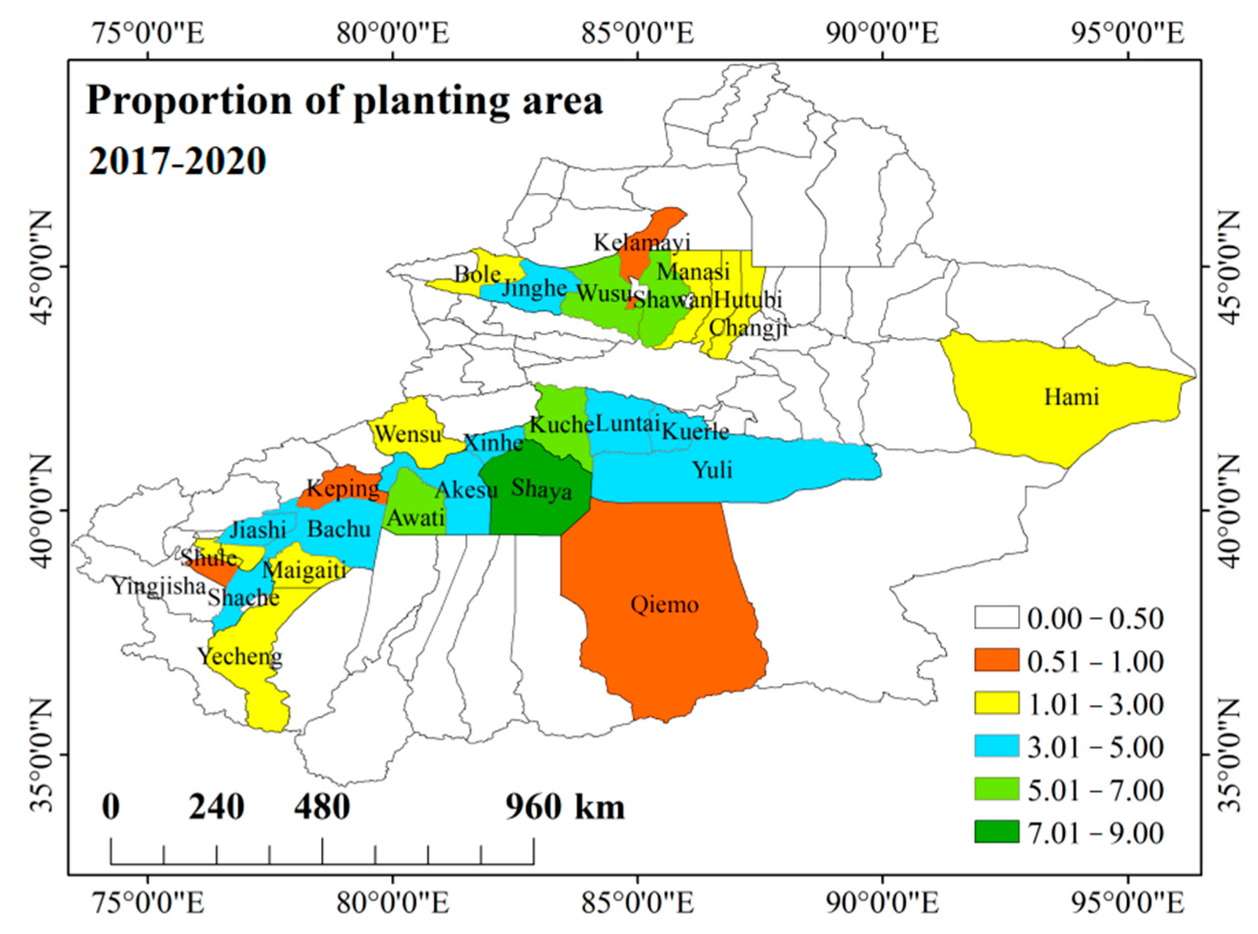
2.1. Study Area and Planting Area Distribution

This study investigated cotton-growing areas in Xinjiang (Figure 1). The cotton planting regions of Xinjiang include 28 major ecological zones (counties). The cotton planting area in each zone is greater than 0.5% of the total area of Xinjiang, ranging from 0.5% to 9%. The cotton planting area of 14 zones is greater than 3%, and that of 4 zones accounted for less than 1%. Shaya County had the highest planting area, followed by Awati, Wusu, and Shawan, at over 5%.

The cotton region of Xinjiang is a temperate continental climate with complex terrain, diverse climate features, and areas of less-cultivated land. The meteorological resources are conducive to cotton production, with sufficient heat, a significant temperature difference between day and night, long hours of sunshine, scarce precipitation, and a dry climate. In addition, the dry climate characteristics and significant temperature difference between day and night can effectively suppress the occurrence of insect pests. According to the water demand of cotton, artificial irrigation is used to ensure the water supply. The advantages of good climate resources have led to the rapid development of cotton production in this area, which has become the world’s main cotton production region.

2.2. Field Experiment

The WOFOST model was chosen to simulate cotton growth and estimate yield in this study. To calibrate and validate the model, field trials were carried out at the experimental irrigation station of Alar City (81°17′56″ E, 40°32′36″ N) in 2019 and 2020. Irrigation was carried out in drip mode with 6 irrigation treatments (W1–W6). The plot area was 166 m², with 3 replicates. In addition to the irrigation water at the time of seedling emergence, irrigation was carried out at the interval of 13 days for emergence and bud stages, every 7 days for flowering and boll stages, and every 9 days for the boll stage. The specific irrigation scheme for W1–W6 treatment is shown in

Table 1. Irrigation scheme (m³/666 m²).

Number	Date	W1	W2	W3	W4	W5	W6
1	2 June	8.0	9.0	10.0	11.0	12.0	13.0
2	15 June	12.0	13.5	15.0	16.5	18.0	19.5
3	28 June	16.0	18.0	20.0	22.0	24.0	26.0
4	5 July	28.0	31.5	35.0	38.5	42.0	45.5
5	12 July	36.0	40.5	45.0	49.5	54.0	58.5
6	19 July	32.0	36.0	40.0	44.0	48.0	52.0
7	26 July	28.0	31.5	35.0	38.5	42.0	45.5
8	2 August	16.0	18.0	20.0	22.0	24.0	26.0
9	9 August	16.0	18.0	20.0	22.0	24.0	26.0
10	18 August	16.0	18.0	20.0	22.0	24.0	26.0
11	27 August	8.0	9.0	10.0	11.0	12.0	13.0
12	5 September	8.0	9.0	10.0	11.0	12.0	13.0
Total		224.0	252.0	280.0	308.0	336.0	364.0

, and the irrigation date was appropriately adjusted according to rainfall and specific growth conditions.

2.3. Field-Observed Data

After sowing, the germination, budding, flowering, boll opening, and maturity dates of cotton were recorded. Photosynthetically active radiation (PAR) and leaf area index (LAI) were measured by a SunScan canopy analyzer (Delta company, Cambridge, UK) every 10 days. Net photosynthetic rate, stomatal conductance, intercellular CO₂ concentration, and transpiration rate were measured by Li6400xt portable photosynthesis tester every 10 days. Samples were taken every 10 days for biomass measurement and 10 times for the growing season. Three cotton plants were selected for each time. The roots, stems, leaves, and fruits were returned to the laboratory and dried to constant weight at 80 °C. The dry weight of each organ was measured. Before and after irrigation, soil samples were taken from 0–100 cm soil depth with a root drill every 20 cm, and soil volume moisture content was measured more than 20 times a year. Soil parameters such as soil holding capacity, bulk density, saturated soil moisture content, soil water response curve, and permeability coefficient were measured by the direct sampling method, and irrigation date and irrigation amount were recorded simultaneously. An automatic weather station was installed in the experimental field regions for long-term meteorological data observations, including measuring daily maximum and minimum temperatures, solar radiation, precipitation, relative humidity, and wind speed, which were used to drive the field-scale cotton growth model. The yield was observed around the middle of October every year.

2.4. Regional Meteorological Data

The spatial distribution of the mean value of the meteorological data used in the study is shown in Figure 2. Weather-driven data for the model were taken from surface weather observatories in the counties, including minimum temperature, maximum temperature, radiation, wind speed at 2 m height, and precipitation. The average temperature and radiation in southern Xinjiang are generally higher than those in northern Xinjiang, whereas the rainfall is lower than that in northern Xinjiang. Wind speed is unevenly distributed.

2.5. WOFOST Model Description and Calibration

The WOFOST model is a mechanism-based crop growth model jointly developed by Wageningen University in the Netherlands and the World Food Research Center [10]. This model uses light interception and CO₂ assimilation as a growth-driving process. A crop phenology development process is used to describe crop growth. The simulated growth process mainly includes crop carbon assimilation, respiration, transpiration, and dry matter distribution. The model has two main application modes [3]. In the latent mode, the crop growth is only determined by temperature and solar radiation, and other growth limiting factors are not considered; crop growth in the water-limited mode is restricted by water availability. The WOFOST model is a universal model that can simulate different types of crops by customizing different parameters. It has strong applicability and is a good tool for various crop simulations under various environmental conditions. Therefore, in this study, the WOFOST model was used for simulating growth and evaluating the regional adaptability of the mulch-free cultivated cotton in Xinjiang.

The WOFOST model requires each cell’s meteorological, soil, cultivar, and management parameters. Before a crop model is used in a given agro-ecological zone, it must be calibrated and evaluated to ensure that the model can accurately simulate the growth process of the crop by explaining the variability of local cultivars. Our study mainly calibrated cultivar parameters using cotton’s phenological development time and biomass parameters measured in the field during the growing season. Calibration and validation details for WOFOST have been reported previously [43]. In the study, field-measured phenological development stages (emergence, flowering, first pods, first seeds, and maturity dates), total aboveground biomass (TAGP), final yield, leaf area index (LAI), and soil moisture (SM) during the entire growing season in 2019 and 2020 were used to finely calibrate and validate the CRI619 cultivar parameters for the WOFOST model to improve model simulation performance, respectively.

2.6. Evaluation of Simulated Performance

The coefficient of determination (R²) and root mean square error (RMSE) were applied to evaluate the performance. In addition, the ratio of performance to deviation (RPD) [46] was determined as an additional evaluation of modeling utility. If the RPD value is more than 2, the model has good prediction ability and is considered adequate for analytical purposes [46].

Their values were calculated by Equations (1)–(3):

$${\mathrm{R}}^2=1-\frac{{{\displaystyle \sum }}_{i=1}^n{\left(y_i-{\tilde{y}}_i\right)}^2}{{{\displaystyle \sum }}_{i=1}^n{\left(y_i-{ \overline{y}}_{i }\right)}^2}$$

(1)

$$\mathrm{RMSE} =\sqrt{\frac{{{\displaystyle \sum }}_{i=1}^n{\left({\tilde{y}}_i-y_i\right)}^2}{n}}$$

(2)

$$\mathrm{RPD}=\frac{\mathrm{SD}}{\mathrm{RMSE}}$$

(3)

where ${\tilde{y}}_i$ represents simulated value,$y_i$ represents measured value, ${\overline{y}}_{i }$is the average value of the measured values, and $n$ is the number of samples. SD is the standard deviation of measured values.

3. Results

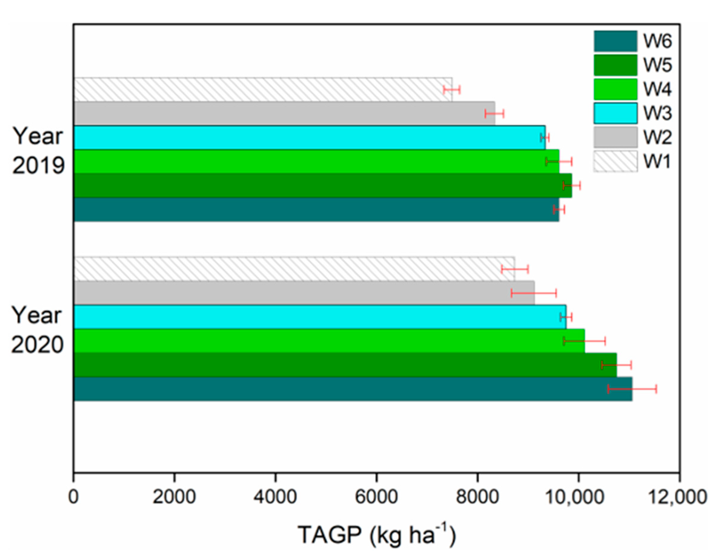
3.1. Significance of Yield and Total Biomass under Different Irrigation Treatments

The yield showed an increasing trend with the increase in irrigation amount in 2019 and 2020, see Figure 3. The highest yields occurred in the W5 treatment, indicating that cotton yield would not continue to increase when irrigation increased to a certain threshold. The yield of W1 and W2, W3 and W4, and W5 and W6 treatments in both years were not significantly different (p > 0.05); see Figure 4.

The TAGP also showed an increasing trend with the increase in irrigation amount in 2019 and 2020 (Figure 5). The highest TAGP appeared in the W5 treatment in 2019 and the W6 treatment in 2020. Higher total biomass was identified in the W6 treatment than in the W5 treatment in 2019, whereas this result was reversed in 2020. The results showed that the highest total biomass does not necessarily have the highest yield, which may be related to the length of cotton fiber growth and accumulation. TAGP of W3W4, W4W5, W4W6, and W5W6 treatments in both years were not significantly different (p > 0.05); see Figure 6.

It is worth noting that when the irrigation strategies and management modes are almost the same, the climate changes significantly impact the yield and TAGP [47]. The average daily temperature for the 2020 cotton growing season was 0.4 °C higher than in 2019, resulting in slightly shorter growing cycles. However, the average daily radiation in 2020 (21,635 kJ m⁻² d⁻¹) was significantly higher than in 2019 (18,168 kJ m⁻² d⁻¹), and the photosynthesis efficiency and organic matter accumulation were more significant in 2020 than in 2019. Hence, the total biomass and yield were slightly higher than in 2019 under the same irrigation treatment conditions.

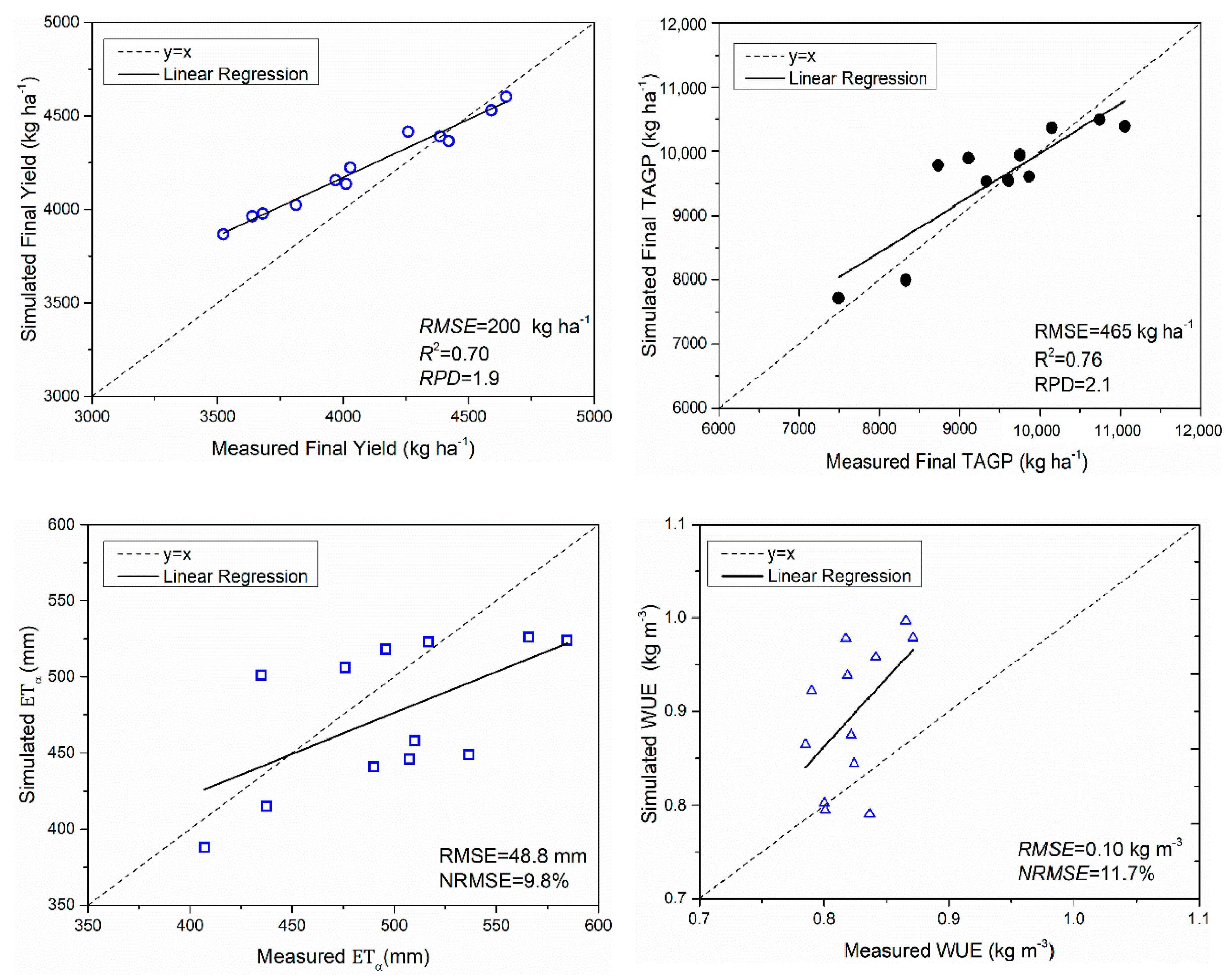
3.2. Calibration and Validation under W6 Treatment

The corrected cotton crop parameters are shown in

Table 2. Calibrated values of the main crop parameters used in the model.

Parameter Name	Description	Value	Units	Source
Emergence parameter
TBASEM	lower threshold temp. for emergence	12	°C
TEFFMX	upper threshold temp. for emergence	30	°C	e
TSUMEM	temperature sum from sowing to emergence	62	°C	m−c
Phenology parameter
TSUM1	temperature sum from emergence to anthesis	750	°C d−1	m−c
TSUM2	temperature sum from anthesis to maturity	1120	°C d−1	m−c
DTSMTB100	effective daily accumulated temperature at an average temperature of 10 °C	0	°C d−1
DTSMTB350	effective daily accumulated temperature at an average temperature of 35 °C	20	°C d−1
Initial parameters
TDWI	initial total crop dry weight	6	kg ha−1	m
LAIEM	leaf area index at emergence	0.004	ha ha−1	m
RGRLAI	maximum relative increase in LAI	0.05	ha ha−1 d−1	m
Green area
SLATB000	specific leaf area when DVS = 0	0.0016	ha kg−1	m−c
SLATB100	specific leaf area when DVS = 1	0.0021	ha kg−1	m−c
SLATB200	specific leaf area when DVS = 2	0.0014	ha kg−1	m−c
SPAN	life span of leaves growing at 35 °C	40	[d]	c
TBASE	lower threshold temp. for the aging of leaves	10	°C
CO2 assimilation
KDIFTB00	extinction coefficient for diffuse visible light when DVS = 0	0.6	\	m−c
KDIFTB200	extinction coefficient for diffuse visible light when DVS = 2	0.6	\	m−c
EFFTB19.5	leaf photosynthesis efficiency at 0 °C	0.40	kg ha−1 hr−1 J−1 m2 s	m−c
EFFTB355	leaf photosynthesis efficiency at 40 °C	0.40	kg ha−1 hr−1 J−1 m2 s	m−c
AMAXTB00	maximum carbon dioxide assimilation rate when DVS = 0	39.0	kg ha−1 hr−1	m−c
AMAXTB170	maximum carbon dioxide assimilation rate when DVS = 1.7	39.0	kg ha−1 hr−1	m−c
AMAXTB200	maximum carbon dioxide assimilation rate when DVS = 2	0	kg ha−1 hr−1	m−c
Conversion of assimilates into biomass
CVL	efficiency of conversion into leaves	0.720	kg kg−1	c
CVO	efficiency of conversion into storage organs	0.610	kg kg−1	c
CVR	efficiency of conversion into roots	0.720	kg kg−1	c
CVS	efficiency of conversion into stems	0.690	kg kg−1	c
Maintenance respiration
Q10	the relative growth rate of respiratory rate for every 10 °C increase in temperature	2	kg CH2O kg−1 d−1	m
RML	relative respiratory rate of leaves	0.0264	kg CH2O kg−1 d−1	m
RMO	relative respiratory rate of fruit	0.035	kg CH2O kg−1 d−1	m
RMR	relative respiratory rate of root	0.038	kg CH2O kg−1 d−1	m
RMS	relative respiratory rate of stem	0.006	kg CH2O kg−1 d−1	m
Partitioning parameters
FLTB	leaf partition coefficient at DVS = 0, 0.9, 1.03, 1.50, 1.85 and 2.00	0.6, 0.4, 0.5, 0.0, 0.0 and 0.0	kg kg−1	m−c
FSTB	stem partition coefficient at DVS = 0, 0.9, 1.03, 1.50, 1.85 and 2.00	0.4, 0.6, 0.5, 0.2, 0.0 and 0.0	kg kg−1	m−c
FOTB	fruit partition coefficient at DVS = 0, 0.9, 1.03, 1.50, 1.85 and 2.00	0.0, 0.0, 0.0, 0.8, 1.0 and 1.0	kg kg−1	m−c
Death rates
RDRSTB00	DVS = 0 relative stem mortality	0.0	\	e
RDRSTB150	DVS = 1.5 relative stem mortality	0.0	\	e
RDRSTB15001	DVS = 1.5001 relative stem mortality	0.02	\	e
RDRSTB200	DVS = 2.0 relative stem mortality	0.02	\	e
Water use
CFET	correction factor transpiration rate	1.0	\	c
DEPNR	crop group number for soil water depletion	1.5	\	c
RDI	initial rooting depth	3	cm	m−c
RRI	the maximum daily increase in rooting depth	0.35	cm d−1	c
RDMCR	maximum rooting depth	60	cm	m−c

based on W6. The parameters were taken from the measured value (m), the corrected value based on the measured value (m−c), the estimated value (e), the corrected value (c), and the reference value from the literature.

Field validation showed that the WOFOST-simulated emergence, flowering, and maturity errors were +1 days, +2 days, and +1 days, respectively, showing good simulation accuracy for phenology development time. The field-verified results of the simulated dry weight of leaves (WLV), stems (WST), storage organs (WSO), and total aboveground production (TAGP) are shown in Figure 7.

Table 3. Validated results for WLV, WST, WSO, and TAGP based on the calibrated model.

	Simulated WLV kg ha−1	Simulated WST kg ha−1	Simulated WSO kg ha−1	Simulated TAGP kg ha−1
RMSE	175	210	199	251
R2	0.96	0.97	0.99	0.99
RPD	5.2	6.3	9.5	16.6

shows that the simulated WLV, WST, WSO, and TAGP agreed well with measured values, with R² = 0.96, 0.97, 0.99, and 0.99, respectively. The RMSE values of simulated versus measured WLV, WST, WSO, and TAGP were 175, 210, 199, and 251 kg ha⁻¹, showing high model accuracy. All RPD values were more than 2, which means that the model had good simulation ability and was considered adequate for analytical purposes [46].

The simulated soil moisture (SM) was in good agreement with the measured value, with R² = 0.89 (Figure 8). The calibration model also showed high simulation accuracy, with RMSE = 0.021 (cm³ cm⁻³). The ratio of RMSE to the mean measured value was approximately 8.6%. The model has good prediction and analytical abilities, with RPD = 3.1, which is higher than 2 [46].

3.3. Validated Results under All Treatments

Measured final yield, TAGP, $E{T}_a$, and WUE for all the treatments were used to evaluate the simulation performance. The scatter plots of the simulated yield, TAGP, $E{T}_a$, and WUE versus measured values were shown in Figure 9. The simulated TAGP and yield agreed well with the measured results, with R² of 0.76 and 0.70, respectively. RMSE values of simulated TAGP and yield were 465 and 200 kg ha^–1, respectively, showing high accuracy. Although the agreement between simulated and measured ETA and WUE was less than 0.1, the percentage RMSE values (ratio of RMSE to the average measured value) of $E{T}_a$ and WUE were, respectively, 9.8% and 11.7%, indicating extremely high precision (NRMSE < 10%) and high precision (10% < NRMSE ≤ 20%), respectively.

In addition, the range of relative bias error (RBE) for the simulated TAGP was from −6.0% to 12.1%, with an average of 1.2% (Figure 10). RBE was almost uniformly distributed. RBE of the simulated yield ranged from −1.3% to 9.7%, with an average of 3.76%. Although most of the samples were slightly overestimated, the errors of the simulated output of different treatments were all within 10%, showing a good yield simulation accuracy. RBE of the simulated $E{T}_a$ ranged from −16.3% to 15.2%, with an average of −4.1%. Most of the samples were slightly underestimated. WUE of the simulated yield ranged from −5.4% to 19.6%, with an average of 8.8%. More samples were slightly overestimated, and the simulation accuracy was slightly lower than that of the other three indexes.

3.4. Evaluation of the Regional Adaptability for Mulch-Free Cultivated Cotton

In this section, the calibrated and validated models are used to evaluate the phenological length, yield, and evapotranspiration of mulch-free cultivated cotton in the main cotton planting regions of Xinjiang, and then to evaluate the adaptability in different regions.

3.4.1. Phenology Length Estimation in Different Regions

The growth period is the growth response of plants to the influence of external ecological factors. The sowing time of CRI619 is usually mid-to-late April. Figure 11 shows the duration of phenological development at different stages in the cotton region of Xinjiang. The development stage (DVS) is an important index to judge whether cotton is mature. The DVS values of Yingjisha and Luntai were lower than 2, so the cotton in these two areas could not mature. Figure 11a shows the phenology time required for cotton from sowing to the emergence of seedlings in various regions. The average seedling emergence time in Keping County was 7.75 days, the average seedling emergence time in Wusu City was 12.75 days, and the seedling emergence time in other counties and cities was within 8–12 days. Figure 11b shows the phenology time required from emergence to flowering. Except for Manasi and Kelamayi, which required 53.25 and 52.75 days, respectively, emergence to flowering was within 54–63 days for other regions. Figure 11c shows the phenology time from flowering to maturity. Wensu and Shule required a longer period for growth and development—101.25 days and 102 days, respectively. In other regions, flowering to maturity was within 62.5–92.5 days. The main reason for the significant differences is probably the meteorological factors in each region. Figure 11d shows the phenology time from emergence to maturity. Wensu and Shule took 162.25 and 165 days, followed by Kuche, Qiemo, Shache, and Xinhe, which took 153.25, 153, 152.25, and 152.25 days, respectively. In other regions, emergence to maturity was between 115.25–149.25 days.

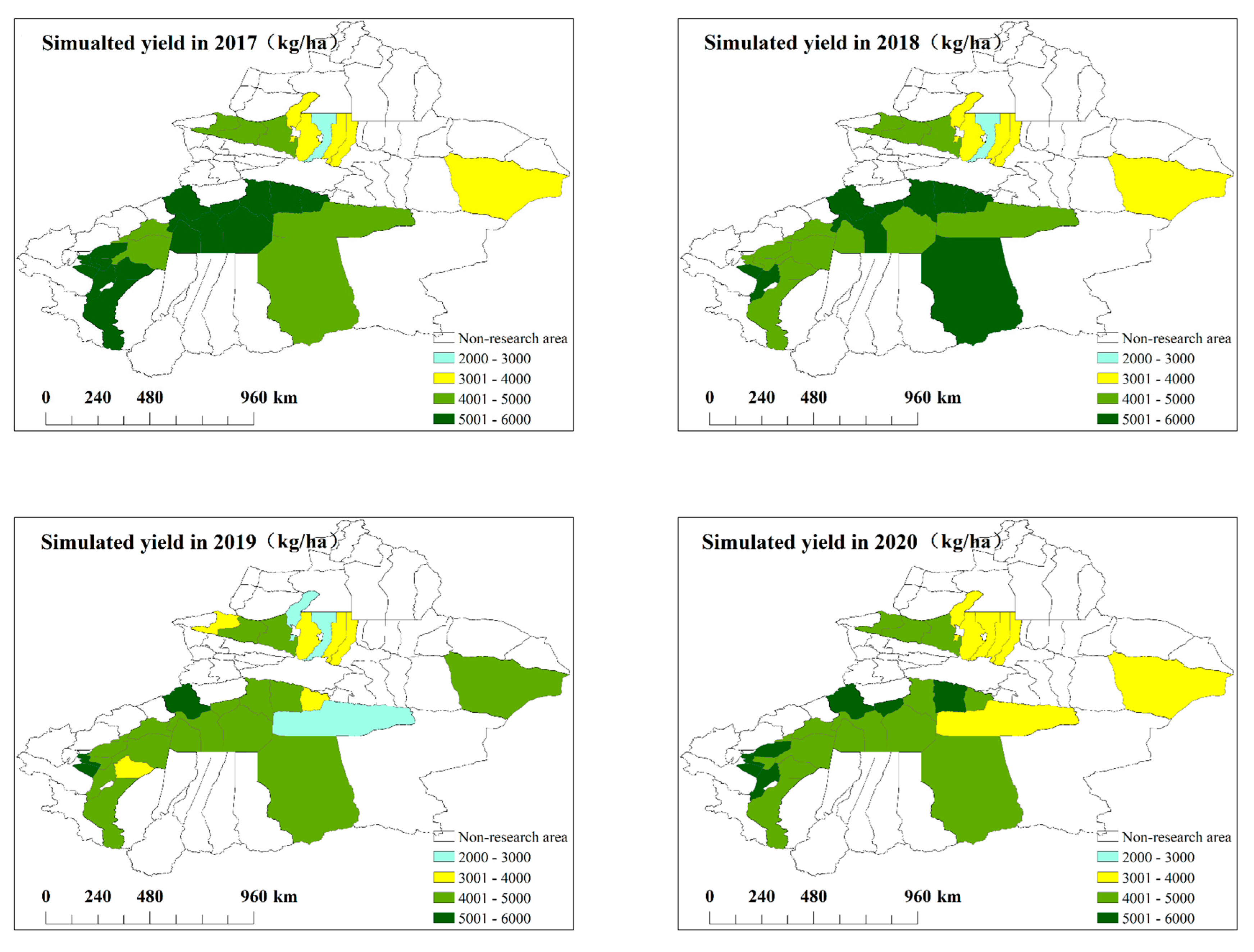
3.4.2. Yield Estimation in Different Regions

Figure 12 provides the geographic distribution of cotton yield from 2017 to 2020 in response to the impact of regional climate variations. Figure 12 shows that, except for the four regions of Bole, Jinghe, Wusu, and Yuli, the output of the southern region of Xinjiang was higher than that of the northern region of Xinjiang. The most critical factors affecting cotton growth are temperature, solar radiation, water, and nutrient supply. In the north, lower solar radiation and temperature are not conducive to cotton growth, but rainfall and irrigation water are sufficient. In the southern region, sufficient sunshine radiation and high temperature can promote the growth of cotton, but the extremely dry and hot weather may cause severe water and heat stress, and rainfall and irrigation water are less abundant than in the northern region.

3.4.3. Evapotranspiration Estimation during the Growth Period in Different Regions

Figure 13 shows the average evapotranspiration for each growth period in the study area from 2017 to 2020. For the Xinjiang cotton region, the evapotranspiration in the south is higher than that in the north. The main reason for this is that the temperature and radiation in the south are generally higher than those in the north (Figure 2), indicating that more irrigation water is needed to ensure the normal growth and development of CRI619 in the southern area.

4. Discussion

4.1. Simulation Performance Analysis of the Calibrated WOFOST Model for Cotton

In the research, the simulated errors of the calibrated WOFOST for emergence, flowering, and maturity were +1 days, +2 days, and +1 days, respectively, showing good simulation accuracy (2.74% error). Existing studies have shown that the average error of phenological development time simulated by calibrated CROPGRO-Cotton in southern Xinjiang is 2.52% [48], which is close to the simulation accuracy of this study. Other research results show that calibrated CROPGRO-Cotton fairly predicts phenological events such as anthesis and physiological maturity with RMSE of ≤2.27 and ≤4.98 d, respectively, in northwestern India [49], and absolute relative errors of 1.7%, 1.1%, and 1.1% based on modified CROPGRO-Cotton. These differences might result from the effects of cotton cultivar and cultivation.

The simulated TAGP and yield agree well with the measured results, with R² of 0.76 and 0.70, and RMSE of 465 and 200 kg ha⁻¹, respectively (Figure 9). AquaCrop is a valuable tool in predicting cotton yield under different irrigation scenarios. The coefficient of determination (R²) in this research is lower than that in the research results of [28] (R² = 0.976 and 0.950), [29] (R² = 0.92 and 0.90), and [21] (R² = 0.92 and 0.90). However, the modeling accuracy is higher than that in the research results of [28] (RMSE = 666 and 999 kg ha⁻¹), [29] (RMSE = 1.19 and 0.25 kg ha⁻¹) and [21] (RMSE = 810 and 751 kg ha⁻¹). CROPGRO-Cotton also shows good prediction performance for TAGP and yield. TAGP and yield exhibit the RMSE of ≤706 and ≤126 kg ha⁻¹, respectively [50].

The simulated soil moisture (SM) is accurate and in good agreement with the measured value, with R² = 0.89 and RMSE = 0.021 (cm³ cm⁻³) (Figure 8), which is higher than the estimation result of the calibrated AquaCrop model, with R² of 0.65 and RMSE of 30.88 mm [29], and the calibrated CROPGRO-Cotton model, with R² of 0.72 and RMSE of 0.087 (cm³ cm⁻³) [51]. However, this result is lower than the research result of [25] based on calibrated AquaCrop, with R² ≥ 0.93 and RMSE ≤ 16.23 mm for the six cotton crop files.

4.2. Uncertainty of the WOFOST Model

When using crop growth models for yield assessment, the uncertainties of input parameters, meteorological driving data, and the simplification of model simulation processes will affect the accuracy of yield estimation [52]. This study simulated the potential crop growth conditions, in which the simulated crops are not affected by water stress, nutrient stress, pests, weeds and other factors, which is very difficult to achieve in the actual planting process. Some studies have confirmed that the TDWI and SPAN parameters strongly influence the initial growth rate of crops and show a high degree of uncertainty, which can affect the growth rate of the initial LAI and the maximum LAI [53]. Although SPAN, which determines the rate and timing of leaf senescence, is a characteristic of crop variety, this parameter may be influenced by nitrogen shortage and pests and diseases [54]. However, the WOFOST model cannot simulate the effects of these factors on SPAN [50].

In addition, the input crop parameters, meteorological parameters, and soil parameters are also uncertain. In the study, the model parameters for the new cotton cultivar CRI619 were calibrated and verified by field experiments. The results show that the corrected model predicted the plant growth and development processes well. Therefore, we used the correction model to simulate the growth and yield formation of CRI619 in different cotton regions. In future research, we can use remote sensing to assimilate the state variables such as soil moisture and leaf area index to correct the soil attribute parameters and crop parameters at a regional scale, and thereby provide a rational simulation model for regional-scale analysis of the effects of non-film cultivation on cotton growth and yield.

4.3. The Influence of Temperature on Phenological Development Length

The phenological development length of cotton is mainly affected by temperature [2]. Figure 11 also confirms that temperature differences in different cotton growing areas lead to significant differences in emergence to maturity dates, and even some areas cannot reach the accumulated temperature for cotton maturities, such as Yingjisha and Luntai counties.

The suitable temperature index for cotton planting is such that the average daily temperature for five consecutive days is above 15 °C [55]. Below this temperature, conditions are not suitable for cotton planting. The average temperatures in April for the seven regions of Bole, Changji, Jinghe, Luntai, Qiemo, and Wusu are below 15 °C. Therefore, it is better to postpone planting to the end of April or the beginning of May.

The higher the daily average temperature after sowing cotton, the shorter the period of seedling emergence. When encountering freezing weather, the intensity and duration of the low temperatures are closely related to the length of time from sowing to the emergence period. When the day’s minimum temperature drops below 10 °C, cold damage will occur, and the emergence time will increase significantly [56]. The lowest temperatures in Akesu, Bole, Changji, Hami, Jinghe, Kuqa, Qiemo, Shaya, Wensu, Wusu, Xinhe, and Yingjisha are all below 10 °C, and cold damage is likely to occur. The average temperature in the five regions of Hami, Hutubi, Kuqa, Shule, and Yingjisha is between 15–16 °C. Therefore, the development is prolonged, as the optimum temperature is 25–30 °C.

Cotton must go through two periods: emergence to budding and budding to flowering. The minimum temperature for development from emergence to budding is 12 °C, the optimum temperature is about 25 °C, and the upper limit temperature is 35 °C [55]. The development time is usually late April or early May to early mid-June. The average temperature in May in all regions is above 19 °C, the highest temperature is around 27 °C, the average temperature in June is around 25 °C, and the highest temperature is around 31 °C. The temperature is highly suitable for the growth and development of cotton. From budding to blooming (usually from mid-to-late June to mid-to-late July), the optimum average temperature is about 25 °C. When the average daily temperature is ≤15 °C, the growth and development of cotton will slow. Similarly, when the daily maximum temperature is ≥35 °C, it will not only cause the shedding of young buds but also reduce the vigor of pollen, affect normal pollination, and reduce the rate of boll setting. The average temperature in June and July is around 25 and 27 °C, respectively. Except for the five areas of Hami, Kelamayi, Manasi, Qiemo, and Shawan, the daily maximum temperature is less than 35 °C.

Cotton must go through a boll-splitting period from flowering to maturity. The period from flowering to splitting usually occurs from mid-to-late July to mid-to-early September. The minimum, maximum, and average temperatures from July to September show a downward trend. The mean average temperature in September dropped to about 19 °C, the mean minimum temperature dropped to about 13 °C, the mean maximum temperature dropped to about 26 °C, and the lowest minimum temperature was 8.6 °C in Qiemo. This reduction in average temperatures usually starts from mid-to-early September to mid-to-early October. The mean minimum temperature in October dropped below 8 °C, and the lowest temperature reached −2.3 °C in Qiemo.

4.4. Simulated Cotton Yield in Different Regions

For the adaptability of CRI619 (Gossypium hirsutum Linn) in different regions, yield is one of the critical evaluation indicators. In this study, we mainly explored the impact of meteorological changes on cotton yield and evaluated the yield changes of the CRI619 cultivar in different planting regions using a calibrated model (Figure 12). The yield of the southern region of Xinjiang is higher than that of the northern region of Xinjiang, which is mainly affected by temperature and solar radiation. Temperature mainly affects phenological developmental length [57], as shown in Figure 11. Generally, a longer phenological time can accumulate more biomass; in particular, the phenological length of the fruit development period is more beneficial to yield accumulation [47]. Average daily radiation directly affects photosynthesis efficiency and organic matter accumulation, and high radiation levels usually contribute positively to yield [36]. In addition, improved crop management techniques and varieties may increase yields in many regions. In practice, soil properties, fertilization, and production management will have essential effects on yield, and these factors are not considered in the simulation process.

4.5. Simulated Evapotranspiration in Different Regions

In the arid and semi-arid regions of Xinjiang, water consumption is also an important indicator for evaluating the adaptability of CRI619. Meteorological factors have a significant influence on the evapotranspiration of cotton. The most influential factors include total solar radiation, temperature, and wind speed, of which total solar radiation is the most critical [40]. Figure 13 shows that the evapotranspiration in the south is higher than that in the north, and is mainly determined by temperature, radiation, and wind speed, as shown by the analysis of the model mechanism [3]. Although the yield in southern Xinjiang is relatively high, the water consumption is also relatively large. In arid regions, the balance between yield and water use should be considered in practice to improve water use efficiency and promote sustainable agricultural development.

4.6. Improvement in Cotton Growth Simulation and Yield, Evapotranspiration Evaluation Performance

Remote sensing assimilation is an optimization method that addresses the regional applicability and versatility of crop modeling, scale issues, application fields, and mechanism and application improvements [52]. Remote sensing can provide essential information about meteorology, vegetation, and soil conditions to simulate crop growth within a region. The data of phenological information, LAI, biomass, leaf nitrogen accumulation, evapotranspiration, and soil moisture can be obtained over a large area [58]. These canopy and soil state variables can be integrated into the crop growth model to reduce the uncertainty of the key input parameters of the crop model and improve the simulation results. According to the cotton growth simulation and yield evaluation method carried out in this study, the initial input parameters having large regional uncertainty in the WOFOST model (such as initial dry weight, phenological development parameters, and photosynthesis parameters) are expected to be corrected. The state variables observed by remote sensing can be used to optimize the accuracy of cotton growth simulation and regional yield evaluation. In addition, it is also expected that deep learning methods can be used to further analyze and improve the uncertainty of the input parameters of crop models [59]. Remote sensing assimilation is also a potential method to improve the uncertainty of model input parameters.

In addition, since the simulation parameters of the model are obtained by adjusting the data of an experimental field, there is still some instability. In the future, crop phenology research will comprise a combination of field test observations, crop models, statistical analysis, and other research methods to further improve research results’ reliability. The response mechanism of crop phenology to climate change effects in different regions is variable; according to the characteristics of phenological changes in different regions, corresponding management measures should be adopted to deal with climate change, which is likely to be one of the main directions for future crop phenology research.

5. Conclusions

In this study, the main crop parameter files and simulation processes of the WOFOST model were corrected and improved, and the daily growth and development processes of cotton’s stem, leaf and storage organ biomass, leaf area index, and transpiration were simulated. After calibrating the model, the simulated results agreed well with measured field data for biomass and soil moisture. The corrected model was used to simulate and analyze the phenological development length, yield distribution, and water demand of cotton growing areas in Xinjiang. The simulated phenological development length and yield distribution well reflected the influence of meteorological factors on the growth and development process and the final yield of CRI619. The simulated water demand thoroughly explained the water demand of CRI619 in different cotton regions. The results showed that, in the Xinjiang cotton region, southern Xinjiang had the more suitable temperature and radiation for the growth and development of CRI619, and more water demand during the whole growth period, and the final yield was significantly higher in the south than in the north. Cotton cannot mature in Yingjisha and Luntai, so CRI619 is unsuitable for planting in these two areas. This research is a promising method for evaluating the adaptability of filmless cultivated cotton in different regions.

References

1. ur Rahman, M.H.; Ahmad, A.; Wang, X.; Wajid, A.; Nasim, W.; Hussain, M.; Ahmad, B.; Ahmad, I.; Ali, Z.; Ishaque, W.; et al. Multi-model projections of future climate and climate change impacts uncertainty assessment for cotton production in Pakistan. Agric. For. Meteorol. 2018, 253–254, 94–113. [Google Scholar] [CrossRef]
2. Jans, Y.; Von Bloh, W.; Schaphoff, S.; Müller, C.; Jans, Y. Global cotton production under climate change-Implications for yield and water consumption. Hydrol. Earth Syst. Sci. 2021, 25, 2027–2044. [Google Scholar] [CrossRef]
3. de Wit, A.; Boogaard, H.; Fumagalli, D.; Janssen, S.; Knapen, R.; van Kraalingen, D.; Supit, I.; van der Wijngaart, R.; van Diepen, K. 25 years of the WOFOST cropping systems model. Agric. Syst. 2019, 168, 154–167. [Google Scholar] [CrossRef]
4. McKinion, J.M.; Baker, D.N.; Whisler, F.D.; Lambert, J.R. Application of the GOSSYM/COMAX system to cotton crop management. Agric. Syst. 1989, 31, 55–65. [Google Scholar] [CrossRef]
5. Wall, G.W.; Amthor, J.S.; Kimball, B.A. COTCO2: A cotton growth simulation model for global change. Agric. For. Meteorol. 1994, 70, 289–342. [Google Scholar] [CrossRef]
6. Hearn, A.B. OZCOT: A simulation model for cotton crop management. Agric. Syst. 1994, 44, 257–299. [Google Scholar] [CrossRef]
7. Pathak, T.B.; Fraisse, C.W.; Jones, J.W.; Messina, C.D.; Hoogenboom, G. Use of global sensitivity analysis for CROPGRO cotton model development. Trans. ASABE 2007, 50, 2295–2302. [Google Scholar] [CrossRef]
8. Jones, J.W.; Hoogenboom, G.; Porter, C.H.; Boote, K.J.; Batchelor, W.D.; Hunt, L.A.; Wilkens, P.W.; Singh, U.; Gijsman, A.J.; Ritchie, J.T. The DSSAT cropping system model. Eur. J. Agron. 2003, 18, 235–265. [Google Scholar] [CrossRef]
9. Williams, J.R.; Jones, C.A.; Kiniry, J.R.; Spanel, D.A. EPIC crop growth model. Trans. Am. Soc. Agric. Eng. 1989, 32, 497–511. [Google Scholar] [CrossRef]
10. van Diepen, C.A.; Wolf, J.; van Keulen, H.; Rappoldt, C. WOFOST: A simulation model of crop production. Soil Use Manag. 1989, 5, 16–24. [Google Scholar] [CrossRef]
11. Stöckle, C.O.; Donatelli, M.; Nelson, R. CropSyst, a cropping systems simulation model. Eur. J. Agron. 2003, 18, 289–307. [Google Scholar] [CrossRef]
12. Steduto, P.; Hsiao, T.C.; Raes, D.; Fereres, E. Aquacrop-the FAO crop model to simulate yield response to water: I. concepts and underlying principles. Agron. J. 2009, 101, 426–437. [Google Scholar] [CrossRef] [Green Version]
13. Thorp, K.R.; Ale, S.; Bange, M.P.; Barnes, E.M.; Hoogenboom, G.; Lascano, R.J.; McCarthy, A.C.; Nair, S.; Paz, J.O.; Rajan, N.; et al. Development and application of process-based simulation models for cotton production: A review of past, present, and future directions. J. Cotton Sci. 2014, 18, 10–47. [Google Scholar]
14. Amin, A.; Nasim, W.; Mubeen, M.; Nadeem, M.; Ali, L.; Hammad, H.M.; Sultana, S.R.; Jabran, K.; ur Rehman, M.H.; Ahmad, S.; et al. Optimizing the phosphorus use in cotton by using CSM-CROPGRO-cotton model for semi-arid climate of Vehari-Punjab, Pakistan. Environ. Sci. Pollut. Res. 2017, 24, 5811–5823. [Google Scholar] [CrossRef]
15. Thorp, K.R.; Hunsaker, D.J.; Bronson, K.F.; Andrade-Sanchez, P.; Barnes, E.M. Cotton irrigation scheduling using a crop growth model and FAO-56 methods: Field and simulation studies. Trans. ASABE 2017, 60, 2023–2039. [Google Scholar] [CrossRef] [Green Version]
16. Li, F.; Yu, D.; Zhao, Y. Irrigation Scheduling Optimization for Cotton Based on the AquaCrop Model. Water Resour. Manag. 2019, 33, 39–55. [Google Scholar] [CrossRef]
17. Abbas, G.; Fatima, Z.; Tariq, M.; Ahmed, M.; ur Rahman, M.H.; Nasim, W.; Rasul, G.; Ahmad, S. Applications of crop modeling in cotton production. In Cotton Production and Uses: Agronomy, Crop Protection, and Postharvest Technologies; Springer: Berlin/Heidelberg, Germany, 2020; ISBN 9789811514722. [Google Scholar]
18. Mahadevappa, S.G.; Sreenivas, G.; Raji Reddy, D.; Madhavi, A.; Rao, S.S. Application of cropgro-cotton model to optimize irrigation scheduling in bt cotton on alfisols of southern telangana. J. Agrometeorol. 2020, 22, 390–393. [Google Scholar] [CrossRef]
19. Ale, S.; Omani, N.; Himanshu, S.K.; Bordovsky, J.P.; Thorp, K.R.; Barnes, E.M. Determining optimum irrigation termination periods for cotton production in the Texas high plains. Trans. ASABE 2020, 63, 105–115. [Google Scholar] [CrossRef]
20. Thorp, K.R.; Thompson, A.L.; Bronson, K.F. Irrigation rate and timing effects on Arizona cotton yield, water productivity, and fiber quality. Agric. Water Manag. 2020, 234, 106146. [Google Scholar] [CrossRef]
21. Wang, X.; Jiang, F.; Wang, H.; Cao, H.; Yang, Y.; Gao, Y. Irrigation Scheduling Optimization of Drip-irrigated without Plastic Film Cotton in South Xinjiang Based on AquaCrop Model. Nongye Jixie Xuebao/Trans. Chin. Soc. Agric. Mach. 2021, 52, 293–301. [Google Scholar] [CrossRef]
22. Shukr, H.H.; Pembleton, K.G.; Zull, A.F.; Cockfield, G.J. Impacts of effects of deficit irrigation strategy on water use efficiency and yield in cotton under different irrigation systems. Agronomy 2021, 11, 231. [Google Scholar] [CrossRef]
23. Amouzou, K.A.; Naab, J.B.; Lamers, J.P.A.; Borgemeister, C.; Becker, M.; Vlek, P.L.G. CROPGRO-Cotton model for determining climate change impacts on yield, water- and N- use efficiencies of cotton in the Dry Savanna of West Africa. Agric. Syst. 2018, 165, 85–96. [Google Scholar] [CrossRef]
24. Luo, Q.; Bange, M.; Johnston, D.; Braunack, M. Cotton crop water use and water use efficiency in a changing climate. Agric. Ecosyst. Environ. 2015, 202, 126–134. [Google Scholar] [CrossRef]
25. Tsakmakis, I.D.; Kokkos, N.P.; Gikas, G.D.; Pisinaras, V.; Hatzigiannakis, E.; Arampatzis, G.; Sylaios, G.K. Evaluation of AquaCrop model simulations of cotton growth under deficit irrigation with an emphasis on root growth and water extraction patterns. Agric. Water Manag. 2019, 213, 419–432. [Google Scholar] [CrossRef]
26. Wang, K.; Su, L.; Wang, Q. Cotton growth model under drip irrigation with film mulching: A case study of Xinjiang, China. Agron. J. 2021, 113, 2417–2436. [Google Scholar] [CrossRef]
27. Himanshu, S.K.; Fan, Y.; Ale, S.; Bordovsky, J. Simulated efficient growth-stage-based deficit irrigation strategies for maximizing cotton yield, crop water productivity and net returns. Agric. Water Manag. 2021, 250, 106840. [Google Scholar] [CrossRef]
28. Aziz, M.; Rizvi, S.A.; Sultan, M.; Bazmi, M.S.A.; Shamshiri, R.R.; Ibrahim, S.M.; Imran, M.A. Simulating Cotton Growth and Productivity Using AquaCrop Model under Deficit Irrigation in a Semi-Arid Climate. Agriculture 2022, 12, 242. [Google Scholar] [CrossRef]
29. Zhang, J.; Li, K.; Gao, Y.; Feng, D.; Zheng, C.; Cao, C.; Sun, J.; Dang, H.; Hamani, A.K.M. Evaluation of saline water irrigation on cotton growth and yield using the AquaCrop crop simulation model. Agric. Water Manag. 2022, 261, 107355. [Google Scholar] [CrossRef]
30. Zurweller, B.A.; Rowland, D.L.; Mulvaney, M.J.; Tillman, B.L.; Migliaccio, K.; Wright, D.; Erickson, J.; Payton, P.; Vellidis, G. Optimizing cotton irrigation and nitrogen management using a soil water balance model and in-season nitrogen applications. Agric. Water Manag. 2019, 216, 306–314. [Google Scholar] [CrossRef]
31. Arshad, M.N.; Ahmad, A.; Wajid, S.A.; Cheema, M.J.M.; Schwartz, M.W. Adapting dssat model for simulation of cotton yield for nitrogen levels and planting dates. Agron. J. 2017, 109, 2639–2648. [Google Scholar] [CrossRef] [Green Version]
32. Lokhande, S.; Reddy, K.R. Quantifying temperature effects on cotton reproductive efficiency and fiber quality. Agron. J. 2014, 106, 1275–1282. [Google Scholar] [CrossRef]
33. Lokhande, S.; Reddy, K.R. Reproductive and fiber quality responses of upland cotton to moisture deficiency. Agron. J. 2014, 106, 1060–1069. [Google Scholar] [CrossRef]
34. Chen, M.; Zhao, W.; Meng, Y.; Chen, B.; Wang, Y.; Zhou, Z.; Oosterhuis, D.M. A model for simulating the cotton (Gossypium hirsutum L.) embryo oil and protein accumulation under varying environmental conditions. F. Crop. Res. 2015, 183, 79–91. [Google Scholar] [CrossRef]
35. Aydın, İ.; Arslan, S. Mechanical properties of cotton shoots for topping. Ind. Crops Prod. 2018, 112, 396–401. [Google Scholar] [CrossRef]
36. Hou, T.Y.; Hao, T.L.; Wang, H.J.; Zhang, Z.; Lü, X. Advances in cotton growth and development modelling and its applications in China. Sci. Agric. Sin. 2021, 54, 1112–1126. [Google Scholar] [CrossRef]
37. Liang, X.Z.; Xu, M.; Gao, W.; Raja Reddy, K.; Kunkel, K.; Schmoldt, D.L.; Samel, A.N. Physical modeling of U.S. cotton yields and climate stresses during 1979 to 2005. Agron. J. 2012, 104, 675–683. [Google Scholar] [CrossRef] [Green Version]
38. ur Rahman, M.H.; Ahmad, A.; Wajid, A.; Hussain, M.; Rasul, F.; Ishaque, W.; Islam, M.A.; Shelia, V.; Awais, M.; Ullah, A.; et al. Application of CSM-CROPGRO-Cotton model for cultivars and optimum planting dates: Evaluation in changing semi-arid climate. F. Crop. Res. 2019, 238, 139–152. [Google Scholar] [CrossRef]
39. Williams, A.; White, N.; Mushtaq, S.; Cockfield, G.; Power, B.; Kouadio, L. Quantifying the response of cotton production in eastern Australia to climate change. Clim. Chang. 2015, 129, 183–196. [Google Scholar] [CrossRef]
40. Voloudakis, D.; Karamanos, A.; Economou, G.; Kalivas, D.; Vahamidis, P.; Kotoulas, V.; Kapsomenakis, J.; Zerefos, C. Prediction of climate change impacts on cotton yields in Greece under eight climatic models using the AquaCrop crop simulation model and discriminant function analysis. Agric. Water Manag. 2015, 147, 116–128. [Google Scholar] [CrossRef]
41. Adhikari, P.; Ale, S.; Bordovsky, J.P.; Thorp, K.R.; Modala, N.R.; Rajan, N.; Barnes, E.M. Simulating future climate change impacts on seed cotton yield in the Texas High Plains using the CSM-CROPGRO-Cotton model. Agric. Water Manag. 2016, 164, 317–330. [Google Scholar] [CrossRef]
42. Luo, Q.; Bange, M.; Braunack, M.; Johnston, D. Effectiveness of agronomic practices in dealing with climate change impacts in the Australian cotton industry—A simulation study. Agric. Syst. 2016, 147, 1–9. [Google Scholar] [CrossRef]
43. Bai, T.; Zhang, N.; Wang, T.; Wang, D.; Yu, C.; Meng, W.; Fei, H.; Chen, R.; Li, Y.; Zhou, B. Simulating on the effects of irrigation on jujube tree growth, evapotranspiration and water use based on crop growth model. Agric. Water Manag. 2021, 243, 106517. [Google Scholar] [CrossRef]
44. Mubeen, M.; Ahmad, A.; Hammad, H.M.; Awais, M.; Farid, H.U.; Saleem, M.; Ul Din, M.S.; Amin, A.; Ali, A.; Fahad, S.; et al. Evaluating the climate change impact on water use efficiency of cotton-wheat in semi-arid conditions using dssat model. J. Water Clim. Chang. 2020, 11, 1661–1675. [Google Scholar] [CrossRef]
45. Himanshu, S.K.; Ale, S.; Bordovsky, J.P.; Kim, J.J.; Samanta, S.; Omani, N.; Barnes, E.M. Assessing the impacts of irrigation termination periods on cotton productivity under strategic deficit irrigation regimes. Sci. Rep. 2021, 11, 20102. [Google Scholar] [CrossRef]
46. Fleming, A.; Schenkel, F.S.; Chen, J.; Malchiodi, F.; Bonfatti, V.; Ali, R.A.; Mallard, B.; Corredig, M.; Miglior, F. Prediction of milk fatty acid content with mid-infrared spectroscopy in Canadian dairy cattle using differently distributed model development sets. J. Dairy Sci. 2017, 100, 5073–5081. [Google Scholar] [CrossRef] [PubMed] [Green Version]
47. Li, N.; Lin, H.; Wang, T.; Li, Y.; Liu, Y.; Chen, X.; Hu, X. Impact of climate change on cotton growth and yields in Xinjiang, China. F. Crop. Res. 2020, 247, 107590. [Google Scholar] [CrossRef]
48. Wang, X.; Wang, H.; Si, Z.; Gao, Y.; Duan, A. Modelling responses of cotton growth and yield to pre-planting soil moisture with the CROPGRO-Cotton model for a mulched drip irrigation system in the Tarim Basin. Agric. Water Manag. 2020, 241, 106378. [Google Scholar] [CrossRef]
49. Mishra, S.K.; Kaur, V.; Singh, K. Evaluation of DSSAT-CROPGRO-cotton model to simulate phenology, growth, and seed cotton yield in northwestern India. Agron. J. 2021, 113, 3975–3990. [Google Scholar] [CrossRef]
50. Curnel, Y.; de Wit, A.J.W.; Duveiller, G.; Defourny, P. Potential performances of remotely sensed LAI assimilation in WOFOST model based on an OSS Experiment. Agric. For. Meteorol. 2011, 151, 1843–1855. [Google Scholar] [CrossRef]
51. Li, M.; Du, Y.; Zhang, F.; Bai, Y.; Fan, J.; Zhang, J.; Chen, S. Simulation of cotton growth and soil water content under film-mulched drip irrigation using modified CSM-CROPGRO-cotton model. Agric. Water Manag. 2019, 218, 124–138. [Google Scholar] [CrossRef]
52. Huang, J.; Gómez-Dans, J.L.; Huang, H.; Ma, H.; Wu, Q.; Lewis, P.E.; Liang, S.; Chen, Z.; Xue, J.H.; Wu, Y.; et al. Assimilation of remote sensing into crop growth models: Current status and perspectives. Agric. For. Meteorol. 2019, 276–277, 107609. [Google Scholar] [CrossRef]
53. Huang, J.; Ma, H.; Su, W.; Zhang, X.; Huang, Y.; Fan, J.; Wu, W. Jointly Assimilating MODIS LAI and et Products into the SWAP Model for Winter Wheat Yield Estimation. IEEE J. Sel. Top. Appl. Earth Obs. Remote Sens. 2015, 8, 4060–4071. [Google Scholar] [CrossRef]
54. Huang, J.; Tian, L.; Liang, S.; Ma, H.; Becker-Reshef, I.; Huang, Y.; Su, W.; Zhang, X.; Zhu, D.; Wu, W. Improving winter wheat yield estimation by assimilation of the leaf area index from Landsat TM and MODIS data into the WOFOST model. Agric. For. Meteorol. 2015, 204, 106–121. [Google Scholar] [CrossRef] [Green Version]
55. Li, N.; Li, Y.; Biswas, A.; Wang, J.; Dong, H.; Chen, J.; Liu, C.; Fan, X. Impact of climate change and crop management on cotton phenology based on statistical analysis in the main-cotton-planting areas of China. J. Clean. Prod. 2021, 298, 126750. [Google Scholar] [CrossRef]
56. Luo, Q.; Bange, M.; Clancy, L. Cotton crop phenology in a new temperature regime. Ecol. Modell. 2014, 285, 22–29. [Google Scholar] [CrossRef]
57. Dhir, A.; Pal, R.K.; Kingra, P.K.; Mishra, S.K.; Sandhu, S.S. Cotton Phenology and production response to sowing time, row orientation and plant spacing using Cropgro-cotton model. Mausam 2021, 72, 627–634. [Google Scholar] [CrossRef]
58. Jin, X.; Kumar, L.; Li, Z.; Feng, H.; Xu, X.; Yang, G.; Wang, J. A review of data assimilation of remote sensing and crop models. Eur. J. Agron. 2018, 92, 141–152. [Google Scholar] [CrossRef]
59. Elavarasan, D.; Durairaj Vincent, P.M. Crop Yield Prediction Using Deep Reinforcement Learning Model for Sustainable Agrarian Applications. IEEE Access 2020, 8, 86886–86901. [Google Scholar] [CrossRef]
Figure 1. Major ecological planting zones for cotton and % area proportion in Xinjiang, China.
Agriculture 12 00895 g001
Figure 2. Mean values of the key meteorological data for major cotton planting zones in Xinjiang from 2017 to 2020.
Agriculture 12 00895 g002
Figure 3. Measured final cotton yield for all irrigation treatments (W1−W6) in 2019 and 2020.
Agriculture 12 00895 g003
Figure 4. Significance of yield under 6 irrigation treatments in 2019 (a) and 2020 (b) (p < 0.05).
Agriculture 12 00895 g004
Figure 5. Measured final total aboveground biomass for all irrigation treatments (W1–W6) in 2019 and 2020.
Agriculture 12 00895 g005
Figure 6. Significance of TAGP under 6 irrigation treatments in 2019 (a) and 2020 (b) (p < 0.05).
Agriculture 12 00895 g006
Figure 7. Verified cotton growth dynamics during the 2019 growth period under W6 irrigation treatment, including the dry weight of leaves (WLV), stems (WST), storage organs (WSO), and total aboveground production (TAGP).
Agriculture 12 00895 g007
Figure 8. Simulated versus measured soil moisture (SM) during the 2019 growth period under W6 irrigation treatment.
Agriculture 12 00895 g008
Figure 9. Simulated versus measured TAGP, yield, E T a , and WUE for six irrigation treatments.
Agriculture 12 00895 g009
Figure 10. Frequency distribution of relative bias error for simulated yield, TAGP ,   E T a , and WUE.
Agriculture 12 00895 g010
Figure 11. Cotton growth period length for different development stages in different regions of Xinjiang, China. (a), from sowing to emergence, (b), from emergence to flowering, (c), from flowering to maturity, (d), from emergence to maturity.
Agriculture 12 00895 g011
Figure 12. Simulated cotton yield in different regions of Xinjiang, China.
Agriculture 12 00895 g012
Figure 13. Simulated evapotranspiration in the main cotton growth period in different regions of Xinjiang, China.
Agriculture 12 00895 g013