
Weed Detection in Maize Fields by UAV Images Based on Crop Row Preprocessing and Improved YOLOv4

 , , , , and
Abstract
:1. Introduction
2. Materials and Methods
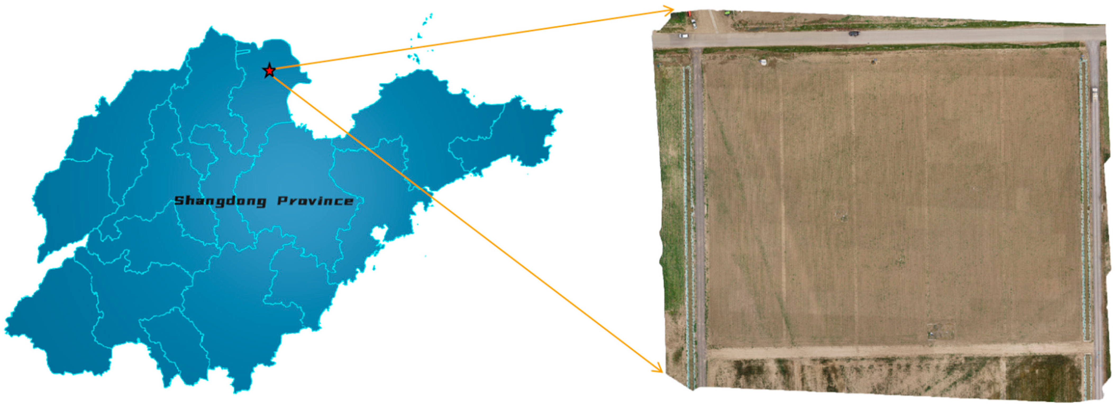
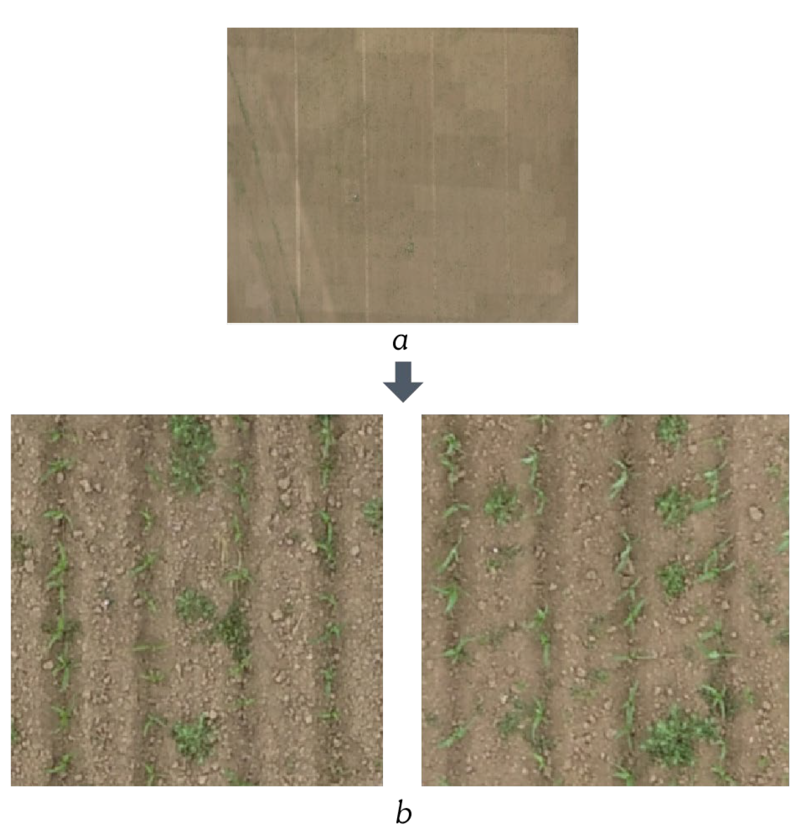
2.1. Data Collection
2.2. YOLOv4 and YOLOv4-Tiny
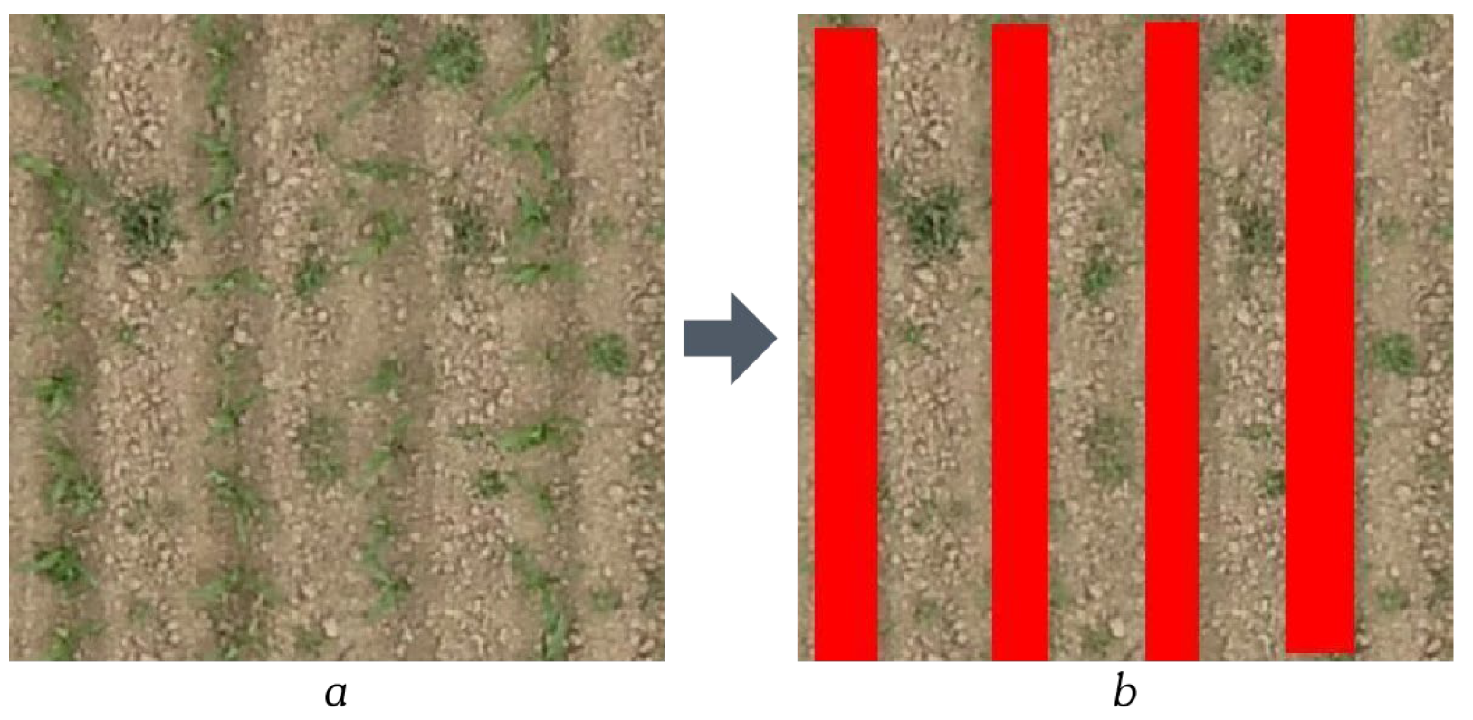
2.3. Crop Row Detection and Mask
2.3.1. Crop Row Detection Model Dataset
2.3.2. Crop Row Detection Model
2.4. Weed Detection Model Dataset
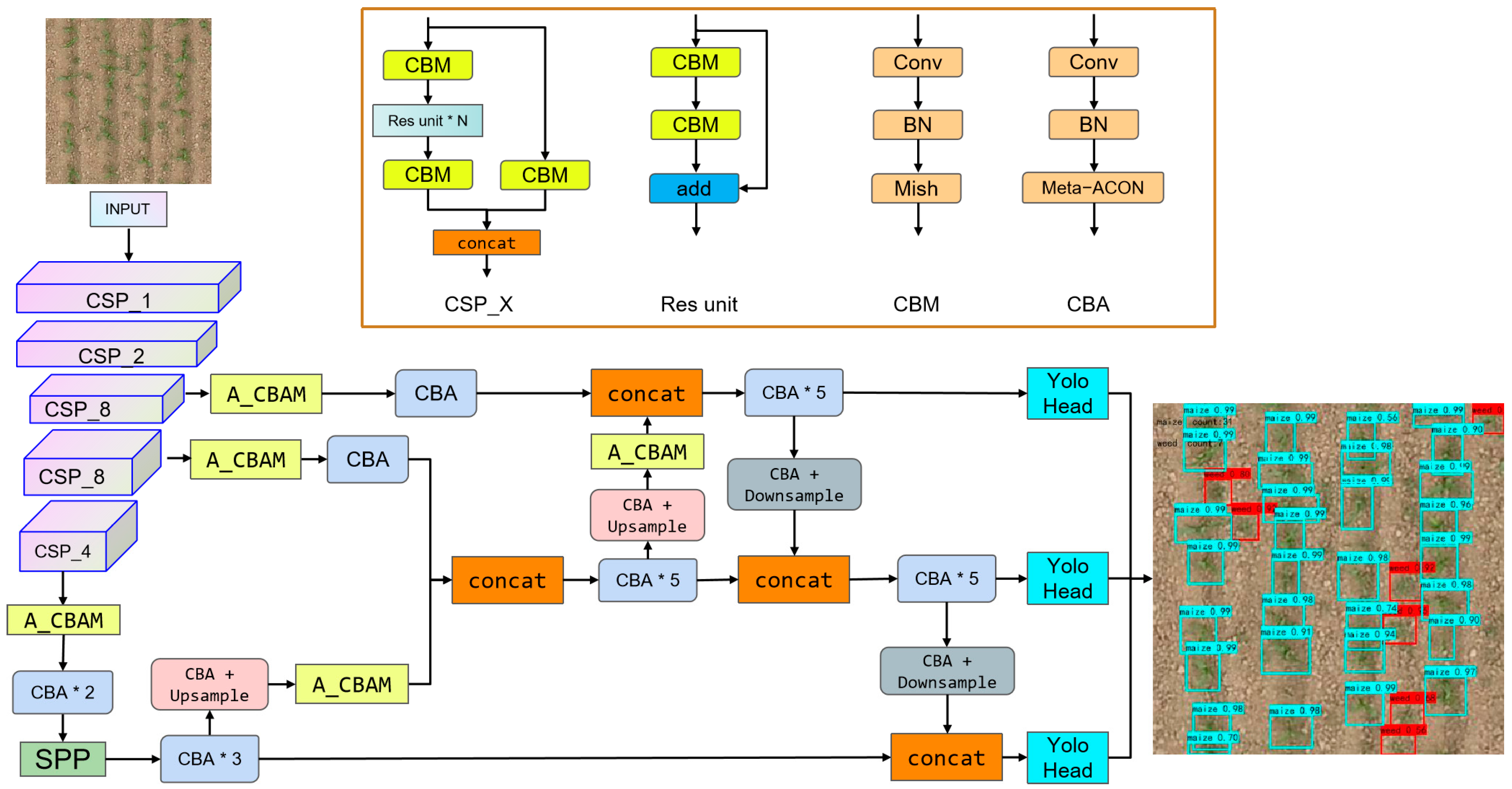
2.5. Weed Detection Model
2.5.1. CBA Module
2.5.2. CBAM
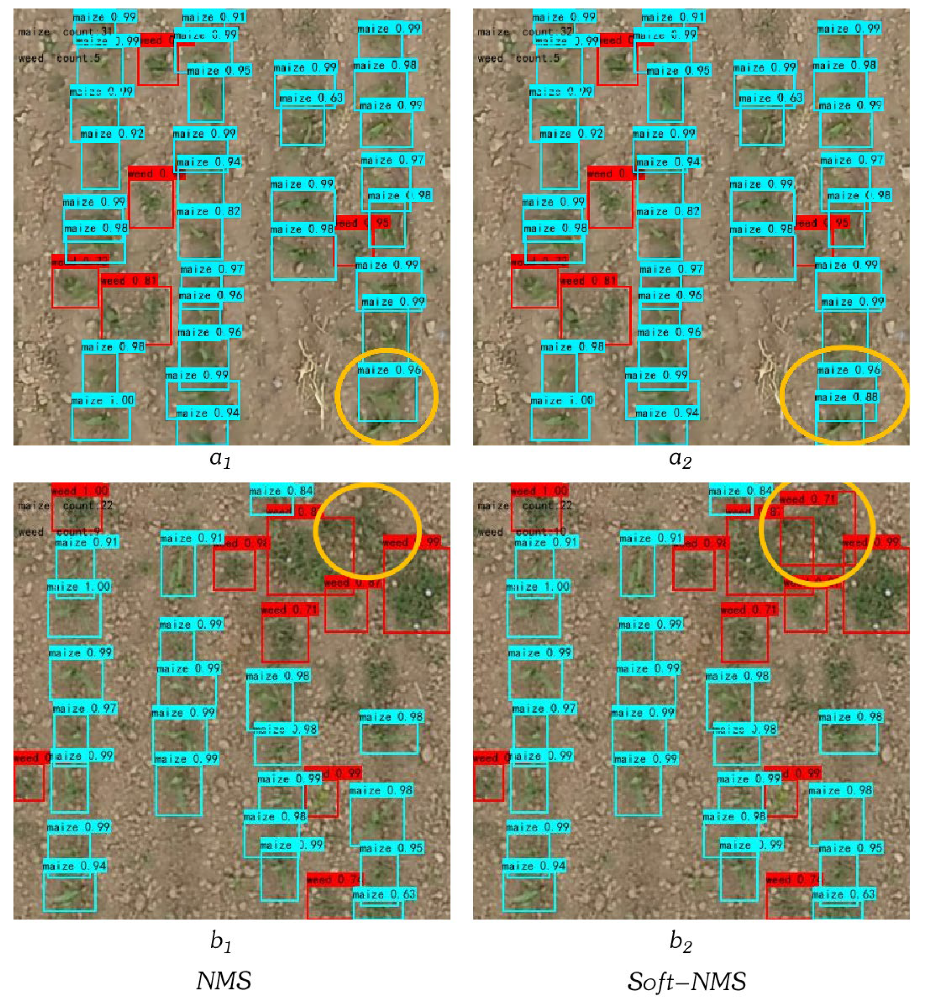
2.5.3. Soft-NMS
2.6. Methods Evaluation Indicator
3. Results and Discussion
3.1. Crop Row Detection Model Experiment
3.2. Weed Detection Model Ablation Experiment
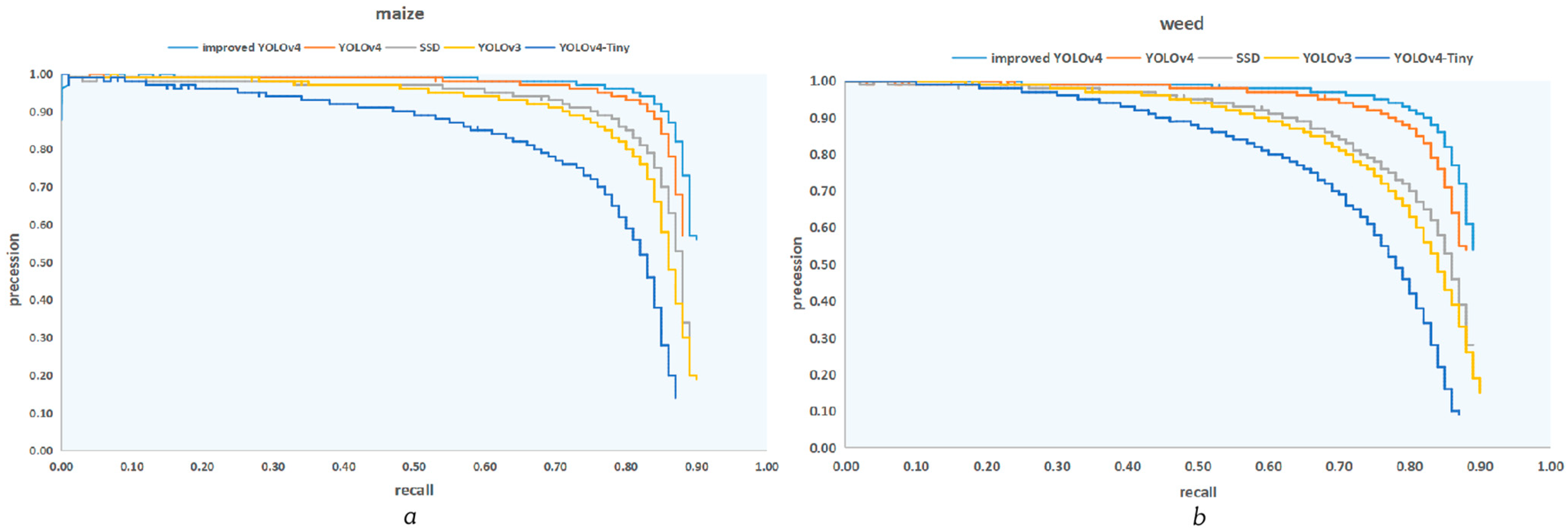
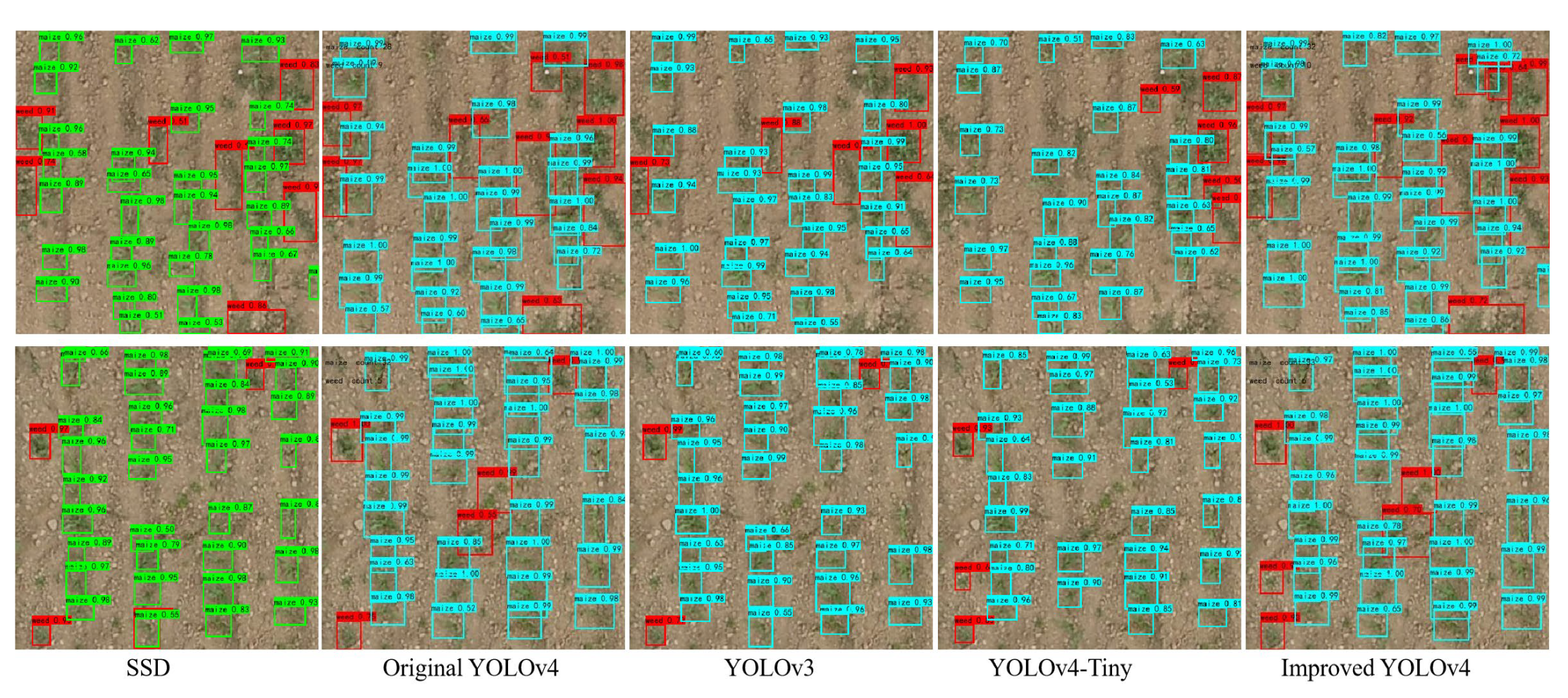
3.3. Weed Detection Model Comparison Experiment
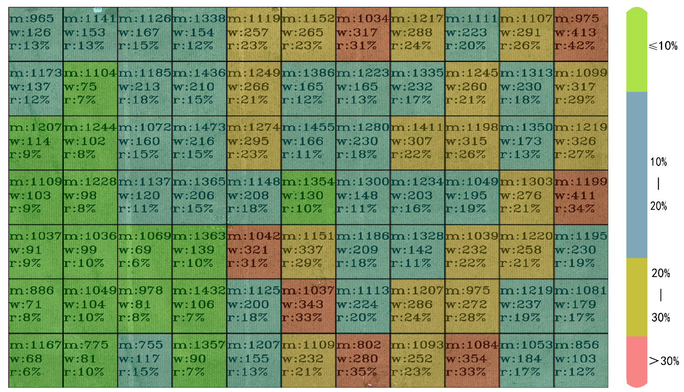
3.4. Maize and Weed Distribution and Counts
3.5. Regional Data Analysis
4. Conclusions
Author Contributions
Funding
Institutional Review Board Statement
Informed Consent Statement
Data Availability Statement
Conflicts of Interest
Appendix A
- (a)
- Meta-ACON
- (b)
- CBAM
- (c)
- Soft-NMS
References
- Zheng, Y.; Zhu, Q.; Huang, M.; Guo, Y.; Qin, J. Maize and weed classification using color indices with support vector data description in outdoor fields. Comput. Electron. Agric. 2017, 141, 215–222. [Google Scholar] [CrossRef]
- Hasan, A.S.M.M.; Sohel, F.; Diepeveen, D.; Laga, H.; Jones, M.G. A survey of deep learning techniques for weed detection from images. Comput. Electron. Agric. 2021, 184, 106067. [Google Scholar] [CrossRef]
- Mohidem, N.A.; Che’Ya, N.N.; Juraimi, A.S.; Ilahi, W.F.F.; Roslim, M.H.M.; Sulaiman, N.; Saberioon, M.; Noor, N.M. How Can Unmanned Aerial Vehicles Be Used for Detecting Weeds in Agricultural Fields? Agriculture 2021, 11, 1004. [Google Scholar] [CrossRef]
- Ramirez, W.; Achanccaray, P.; Mendoza, L.F.; Pacheco, M.A.C. Deep convolutional neural networks for weed detection in agricultural crops using optical aerial images. In Proceedings of the 2020 IEEE Latin American GRSS & ISPRS Remote Sensing Conference (LAGIRS), Santiago, Chile, 22–26 March 2020. [Google Scholar] [CrossRef]
- Etienne, A.; Ahmad, A.; Aggarwal, V.; Saraswat, D. Deep Learning-Based Object Detection System for Identifying Weeds Using UAS Imagery. Remote Sens. 2021, 13, 5182. [Google Scholar] [CrossRef]
- Ahmad, A.; Ordoñez, J.; Cartujo, P.; Martos, V. Remotely Piloted Aircraft (RPA) in Agriculture: A Pursuit of Sustainability. Agronomy 2020, 11, 7. [Google Scholar] [CrossRef]
- Olson, D.; Anderson, J. Review on unmanned aerial vehicles, remote sensors, imagery processing, and their applications in agriculture. Agron. J. 2021, 113, 971–992. [Google Scholar] [CrossRef]
- Ganesan, R.; Raajini, X.M.; Nayyar, A.; Sanjeevikumar, P.; Hossain, E.; Ertas, A.H. BOLD: Bio-Inspired Optimized Leader Election for Multiple Drones. Sensors 2020, 20, 3134. [Google Scholar] [CrossRef]
- Yayli, U.C.; Kimet, C.; Duru, A.; Cetir, O.; Torun, U.; Aydogan, A.C.; Padmanaban, S.; Ertas, A.H. Design optimization of a fixed wing aircraft. Adv. Aircr. Spacecr. Sci. 2017, 4, 65–80. [Google Scholar] [CrossRef]
- De Castro, A.; Shi, Y.; Maja, J.; Peña, J. UAVs for Vegetation Monitoring: Overview and Recent Scientific Contributions. Remote Sens. 2021, 13, 2139. [Google Scholar] [CrossRef]
- Guo, X.; Liu, Q.; Sharma, R.P.; Chen, Q.; Ye, Q.; Tang, S.; Fu, L. Tree Recognition on the Plantation Using UAV Images with Ultrahigh Spatial Resolution in a Complex Environment. Remote Sens. 2021, 13, 4122. [Google Scholar] [CrossRef]
- Huang, Y.; Reddy, K.N.; Fletcher, R.S.; Pennington, D. UAV low-altitude remote sensing for precision weed management. Weed Technol. 2017, 32, 2–6. [Google Scholar] [CrossRef]
- Somerville, G.J.; Mathiassen, S.K.; Melander, B.; Bøjer, O.M.; Jørgensen, R.N. Analysing the number of images needed to create robust variable spray maps. Precis. Agric. 2021, 22, 1377–1396. [Google Scholar] [CrossRef]
- Kamath, R.; Balachandra, M.; Prabhu, S. Crop and weed discrimination using laws’ texture masks. Int. J. Agric. Biol. Eng. 2020, 13, 191–197. [Google Scholar] [CrossRef]
- Lottes, P.; Khanna, R.; Pfeifer, J.; Siegwart, R.; Stachniss, C. UAV-based crop and weed classification for smart farming. In Proceedings of the 2017 IEEE International Conference on Robotics and Automation (ICRA), Singapore, 3 June 2017. [Google Scholar]
- Islam, N.; Rashid, M.; Wibowo, S.; Xu, C.-Y.; Morshed, A.; Wasimi, S.; Moore, S.; Rahman, S. Early Weed Detection Using Image Processing and Machine Learning Techniques in an Australian Chilli Farm. Agriculture 2021, 11, 387. [Google Scholar] [CrossRef]
- Wang, D.; He, D. Channel pruned YOLO V5s-based deep learning approach for rapid and accurate apple fruitlet detection before fruit thinning. Biosyst. Eng. 2021, 210, 271–281. [Google Scholar] [CrossRef]
- Jabir, B.; Falih, N. A New Hybrid Model of Deep Learning ResNeXt-SVM for Weed Detection. Int. J. Intell. Inf. Technol. 2022, 18, 1–18. [Google Scholar] [CrossRef]
- Hu, K.; Coleman, G.; Zeng, S.; Wang, Z.; Walsh, M. Graph weeds net: A graph-based deep learning method for weed recognition. Comput. Electron. Agric. 2020, 174, 105520. [Google Scholar] [CrossRef]
- Redmon, J.; Farhadi, A. Yolov3: An incremental improvement. arXiv 2018, arXiv:1804.02767. [Google Scholar]
- Bochkovskiy, A.; Wang, C.Y.; Liao, H. Yolov4: Optimal speed and accuracy of object detection. arXiv 2020, arXiv:2004.10934. [Google Scholar]
- Liu, W.; Anguelov, D.; Erhan, D.; Szegedy, C.; Reed, S.E.; Fu, C.; Berg, A.C. SSD: Single Shot MultiBox Detector. arXiv 2015, arXiv:1512.02325. [Google Scholar]
- Ren, S.; He, K.; Girshick, R.; Sun, J. Faster R-CNN: Towards Real-Time Object Detection with Region Proposal Networks. IEEE Trans. Pattern Anal. Mach. Intell. 2017, 39, 1137–1149. [Google Scholar] [CrossRef] [Green Version]
- Sun, J. Activate or Not: Learning Customized Activation [DB/OL]. 2020. Available online: https://doc.paperpass.com/foreign/arXiv200904759.html (accessed on 26 April 2022).
- Kweon, I.S. CBAM: Convolutional Block Attention Module [DB/OL]. 2018. Available online: https://doc.paperpass.com/foreign/arXiv180706521.html (accessed on 26 April 2022).
- Bodla, N.; Singh, B.; Chellappa, R.; Davis, L.S. Soft-NMS—Improving Object Detection with One Line of Code. In Proceeding of the 2017 IEEE International Conference on Computer Vision (ICCV), Venice, Italy, 22–29 October 2017; pp. 5562–5570. [Google Scholar]
- Pix4d. Available online: https://www.pix4d.com/ (accessed on 26 April 2022).
- Junsong, R.; Yi, W. Overview of Object Detection Algorithms Using Convolutional Neural Networks. J. Comput. Commun. 2022, 10, 115–132. [Google Scholar] [CrossRef]
- Li, X.; Du, Y.; Yao, L.; Wu, J.; Liu, L. Design and Experiment of a Broken Corn Kernel Detection Device Based on the Yolov4-Tiny Algorithm. Agriculture 2021, 11, 1238. [Google Scholar] [CrossRef]
- Li, X.; Pan, J.; Xie, F.; Zeng, J.; Li, Q.; Huang, X.; Liu, D.; Wang, X. Fast and accurate green pepper detection in complex backgrounds via an improved Yolov4-tiny model. Comput. Electron. Agric. 2021, 191, 106503. [Google Scholar] [CrossRef]
- Howard, A.G. MobileNets: Efficient Convolutional Neural Networks for Mobile Vision Applications [DB/OL]. 2017. Available online: https://doc.paperpass.com/foreign/arXiv170404861.html (accessed on 26 April 2022).
- Howard, A.; Sandler, M.; Chu, G.; Chen, L.; Chen, B.; Tan, M.; Adam, H. Searching for MobileNetV3. In Proceedings of the IEEE/CVF International Conference on Computer Vision (ICCV), Seoul, Korea, 27 October–2 December 2019. [Google Scholar]
- Han, K.; Wang, Y.; Tian, Q.; Guo, J.; Xu, C.; Xu, C. GhostNet: More features from cheap operations. In Proceedings of the IEEE/CVF Conference on Computer Vision and Pattern Recognition (CVPR), Seattle, WA, USA, 14–19 June 2020. [Google Scholar] [CrossRef]
- LabelImg. Available online: https://github.com/tzutalin/labelImg (accessed on 26 April 2022).
- Neubeck, A.; Van Gool, L. Efficient Non-Maximum Suppression. International Conference on Pattern Recognition. IEEE Comput. Soc. 2006, 3, 850–855. [Google Scholar]
- Djaman, K.; Allen, S.; Djaman, D.S.; Koudahe, K.; Irmak, S.; Puppala, N.; Darapuneni, M.K.; Angadi, S.V. Planting date and plant density effects on maize growth, yield and water use efficiency. Environ. Chall. 2021, 6, 100417. [Google Scholar] [CrossRef]
- Kiss, T.; Balla, K.; Bányai, J.; Veisz, O.; Karsai, I. Associations between plant density and yield components using different sowing times in wheat (Triticum aestivum L.). Cereal Res. Commun. 2018, 46, 211–220. [Google Scholar] [CrossRef]
- Jocher, G.; Stoken, A.; Borovec, J.; Liu, C.; Hogan, A.; Diaconu, L.; Poznanski, J.; Ferriday, R.; Sullivan, T.; Wang, X.; et al. Ul-tralytics/yolov5: v4.0. 2020. Available online: https://zenodo.org/record/3983579#.YsVRg4RBxPY (accessed on 26 April 2022).


| Model | AP | Precision | Recall | FPS | Weight | Parameter |
|---|---|---|---|---|---|---|
| YOLOv4-Mobilenet v1 | 90.19% | 98.03% | 89.52% | 20.78 | 53.6 MB | 48.42 MB |
| YOLOv4-Mobilenet v3 | 92.81% | 98.12% | 89.16% | 18.91 | 56.4 MB | 44.74 MB |
| YOLOv4-Ghost | 92.56% | 98.59% | 90.28% | 16.04 | 44.5 MB | 43.60 MB |
| YOLOv4 | 93.15% | 98.06% | 90.77% | 18.53 | 256.3 MB | 245.53 MB |
| YOLOv4-Tiny | 92.97% | 99.28% | 89.74% | 42.24 | 23.6 MB | 23.10 MB |
| Parameters | YOLOv4- Mobilenet v1 | YOLOv4- Mobilenet v3 | YOLOv4- Ghost | YOLOv4 | YOLOv4-Tiny |
|---|---|---|---|---|---|
| Batch size = 4 Epochs = 50 | 39 m 48 s | 49 m 48 s | 56 m 48 s | 92 m 08 s | 10 m 45 s |
| Batch size = 4 Epochs = 100 | 78 m 37 s | 102 m 31 s | 113 m 26 s | 181 m 19 s | 21 m 29 s |
| Batch size = 4 Epochs = 200 | 154 m 47 s | 204 m 48 s | 215 m 39 s | 349 m 48 s | 42 m 23 s |
| Batch size = 8 Epochs = 50 | 11 m 30 s | 13 m 17 s | 14 m 45 s | 19 m 43 s | 8 m 36 s |
| Batch size = 8 Epochs = 100 | 22 m 31 s | 25 m 28 s | 29 m 30 s | 38 m 35 s | 17 m 08 s |
| Batch size = 8 Epochs = 200 | 48 m 29 s | 48 m 09 s | 48 m 14 s | 75 m 57 s | 33 m 05 s |
| Batch size = 16 Epochs = 50 | 11 m 05 s | 11 m 30 s | 12 m 08 s | 17 m 10 s | 8 m 18 s |
| Batch size = 16 Epochs = 100 | 22 m 13 s | 22 m 30 s | 24 m 01 s | 34 m 15 s | 16 m 33 s |
| Batch size = 16 Epochs = 200 | 48 m 30 s | 47 m 45 s | 47 m 20 s | 67 m 33 s | 32 m 31 s |
| Model | mAP | AP | Recall | Precision | |||
|---|---|---|---|---|---|---|---|
| Maize | Weed | Maize | Weed | Maize | Weed | ||
| Original YOLO-v4 | 84.96% | 85.97% | 83.94% | 81.49% | 73.80% | 92.60% | 92.71% |
| YOLOv4+CBA | 85.75% | 86.67% | 84.83% | 83.25% | 77.95% | 92.51% | 92.69% |
| Model | Position | mAP | AP | Recall | Precision | |||
|---|---|---|---|---|---|---|---|---|
| Maize | Weed | Maize | Weed | Maize | Weed | |||
| Original YOLOv4 | 84.96% | 85.97% | 83.94% | 81.49% | 73.80% | 92.60% | 92.71% | |
| CBAM | effective feature layers | 85.10% | 86.13% | 84.07% | 81.53% | 74.69% | 92.59% | 92.53% |
| A_CBAM | 85.31% | 86.18% | 84.45% | 82.42% | 74.58% | 90.97% | 92.78% | |
| CBAM | upsampling | 85.32% | 86.52% | 84.12% | 81.87% | 72.03% | 92.09% | 93.86% |
| A_CBAM | 85.49% | 86.44% | 84.55% | 82.23% | 75.59% | 92.17% | 93.46% | |
| CBAM | effective feature layers +upsampling | 85.77% | 86.82% | 84.72% | 81.44% | 72.09% | 93.73% | 94.63% |
| A_CBAM | 86.08% | 87.08% | 85.08% | 82.37% | 73.77% | 93.15% | 94.25% | |
| Model | mAP | AP | Recall | Precision | F1 | ||||
|---|---|---|---|---|---|---|---|---|---|
| Maize | Weed | Maize | Weed | Maize | Weed | Maize | Weed | ||
| Original YOLOv4 | 84.96% | 85.97% | 83.94% | 81.49% | 73.80% | 92.60% | 92.71% | 87% | 82% |
| SSD | 81.76% | 83.42% | 80.10% | 78.59% | 69.36% | 87.55% | 85.07% | 83% | 76% |
| YOLOv3 | 80.55% | 82.32% | 78.79% | 72.77% | 63.05% | 89.13% | 87.53% | 80% | 73% |
| YOLOv4-Tiny | 73.24% | 74.56% | 71.93% | 67.97% | 56.02% | 79.39% | 83.98% | 73% | 67% |
| Improved YOLOv4 | 86.89% | 87.49% | 86.28% | 83.55% | 78.02% | 93.50% | 93.98% | 88% | 85% |
Publisher’s Note: MDPI stays neutral with regard to jurisdictional claims in published maps and institutional affiliations. |
© 2022 by the authors. Licensee MDPI, Basel, Switzerland. This article is an open access article distributed under the terms and conditions of the Creative Commons Attribution (CC BY) license (https://creativecommons.org/licenses/by/4.0/).
Share and Cite
Pei, H.; Sun, Y.; Huang, H.; Zhang, W.; Sheng, J.; Zhang, Z. Weed Detection in Maize Fields by UAV Images Based on Crop Row Preprocessing and Improved YOLOv4. Agriculture 2022, 12, 975. https://doi.org/10.3390/agriculture12070975
Pei H, Sun Y, Huang H, Zhang W, Sheng J, Zhang Z. Weed Detection in Maize Fields by UAV Images Based on Crop Row Preprocessing and Improved YOLOv4. Agriculture. 2022; 12(7):975. https://doi.org/10.3390/agriculture12070975
Chicago/Turabian StylePei, Haotian, Youqiang Sun, He Huang, Wei Zhang, Jiajia Sheng, and Zhiying Zhang. 2022. "Weed Detection in Maize Fields by UAV Images Based on Crop Row Preprocessing and Improved YOLOv4" Agriculture 12, no. 7: 975. https://doi.org/10.3390/agriculture12070975