Abstract
Plant disease detection is essential for optimizing agricultural productivity and crop quality. With the recent advent of deep learning and large-scale plant disease datasets, many studies have shown high performance of supervised learning-based plant disease detectors. However, these studies still have limitations due to two aspects. First, labeling cost and class imbalance problems remain challenging in supervised learning-based methods. Second, plant disease datasets are either unstructured or weakly-unstructured and the shapes of leaves and diseased areas on them are variable, rendering plant disease detection even more challenging. To overcome these limitations, we propose an instance-aware unsupervised plant disease detector, which leverages normalizing flows, a visual saliency map and positional encodings. A novel way to explicitly combine these methods is the proposed model, in which the focus is on reducing background noise. In addition, to better fit the model to the plant disease detection domain and to enhance feature representation, a feature extractor is pre-trained in a self-supervised learning manner using only unlabeled data. In our extensive experiments, it is shown that the proposed approach achieves state-of-the-art performance on widely-used datasets, such as BRACOL (Weakly-unstructured) and PlantVillage (Unstructured), regardless of whether the dataset is weakly-structured or unstructured.
1. Introduction
Plant disease management [1,2,3] plays an important role in optimizing agricultural productivity and increasing quality of crops. However, it is almost impossible to prevent diseases in the early stages owing to numerous potential reasons for diseases, such as pests, insects, pathogens, contaminated soil, and abiotic factors (weed growth, salinity, drought, waterlogging, etc.). Therefore, cultivators are encouraged to periodically monitor crops [4,5] to prevent significant losses caused by plant diseases; however, monitoring farmland is usually labor-intensive and must be conducted on a daily basis. For this reason, approaches to adequately automate the process [6,7,8], namely plant disease detection, have been actively discussed among scientists.
In recent years, there have been many attempts to apply deep learning to plant disease detection [9,10,11,12]; these approaches mainly use a convolutional neural network (CNN), which can effectively take spatial and semantic information into account at the image level. To be precise, they use a CNN-based feature extractor to obtain n-dimensional feature vectors that can explicitly represent spatial and semantic information of input images; the feature extractor is trained in such a way as to maximize distinctions among embedding vectors from different classes. In other words, the feature extractor learns to optimize learnable parameters to reduce error between predictions and corresponding ground truth labels. These CNN-based methods achieve promising performance on plant disease datasets, such as BRACOL [13] and PlantVillage [14], and show the potential of autonomous plant disease detection.
However, these methods are based on supervised learning. This makes them difficult to use in real-world conditions because they are not only dependent on the number of training data but on data quality [15,16]. For example, there are numerous types of plant diseases, such as mildew, wilt, mosaic virus, and rust, and their shapes vary greatly depending on circumstances. In addition, ambiguous boundaries of diseased areas on plants and long growth cycles render plant disease detection even more challenging [17,18,19]. Even if a dataset considering all these cases is acquired, supervised-learning-based CNN models tend to be overfitted to a dominant class due to the class imbalance problem [20,21] between class categories, which deteriorates the ability of feature presentation and may result in redundant performance for classes with relatively fewer training data than that of the dominant class. Therefore, research on unsupervised-learning-based plant disease detection that does not require a labeling process and has the advantage of detecting unseen diseases in the training phase has been in high demand.
Unsupervised plant disease detection can also be referred to as unsupervised anomaly detection for plants because its objective is to identify anomalous areas on plants; and unsupervised anomaly detection can be largely categorized into three groups depending on the characteristics of the dataset, as follows: (1) structured; (2) weakly-unstructured; (3) unstructured. One example of a structured dataset is MVTec-AD [22] which comprises zoomed-in images of fixed shape objects with and without defects that can be commonly found in the manufacturing industry; there has been a lot of research, actively conducted on this benchmark dataset. Thomas D. et al. propose PaDiM [23], which uses a pre-trained feature extractor to obtain embedding vectors at a patch level and clusters the embedding vectors to determine whether they are anomalous. Rudolph et al. [24] introduce a novel way to leverage normalizing flows with multi-scale features. They first apply some augmentation techniques to obtain multi-scale inputs and feed them into a pre-trained feature extractor. Then the extracted embedding vectors are fed into normalizing flows to determine whether the image contains anomalous areas. This approach achieved impressive results on the MVTec-AD dataset. However, the previously mentioned approaches use only structured data, whilst datasets for plant disease detection, such as BRACOL and PlantVillage, to some extent contain unstructured data, in which the shapes of leaves vary even in the same class category. Therefore, directly applying methods that are used in the MVTec-AD dataset to plant disease detection may result in performance degradation.
In this paper, we address the aforementioned problems and propose a novel instance-aware plant disease detector (IA-PDD). Specifically, we propose a novel way to exploit spatial information by combining a saliency map and positional encodings using combined vectors as conditional vectors of normalizing flows. This allows the flow model to achieve an instance-aware property. In addition, we adopt a self-supervised pre-training strategy to overcome the problem that occurs in ImageNet pre-trained feature extractors. That is, ImageNet pre-trained feature extractors tend to be overly sensitive to general changes, such as illumination changes, shadows, etc., rather than only focusing on plant diseases. In our extensive experiments, it is shown that the proposed approach outperforms state-of-the-art methods, such as PaDiM, PatchCore, and CFLOW-AD [25], and achieves the best performance with respect to AUROC on widely used datasets, such as BRACOL (Weakly-unstructured) and PlantVillage (Unstructured), regardless of the characteristic of the datasets.
The contributions of the paper are three-fold, as follows: (1) We propose a novel instance-aware unsupervised plant disease detector, that adaptively leverages normalizing flows, a visual saliency map, and positional encodings; (2) The proposed approach achieves state-of-the-art performance on widely-used datasets, such as BRACOL (Weakly-unstructured) and PlantVillage (Unstructured), regardless of the dataset characteristic; (3) In extensive experiments, we show the efficacy of the proposed method by comparing results depending on methods to pre-train the feature extractor and the number of coupling and pooling layers.
2. Related Works
In this section, we will discuss related works ranging from normalizing flows, which is the main concept used in the paper, to anomaly detection in general. Following a discussion of anomaly detection in an industrial setting, we will focus on anomaly detection for plant disease detection, which is the primary topic of this paper.
2.1. Normalizing Flows
Normalizing flows (NF) [26] are neural networks designed for constructing complex distributions; they work by transforming a probability density through a sequence of invertible and differentiable mappings. The notable characteristic of NFs is that mappings are bijective and reversible. In other words, mappings can be conducted in both forward and backward paths. In addition, unlike commonly-used deterministic generative models, such as generative adversarial networks (GANs) [27], NF has a stochastic characteristic that maps complex data distribution to simple distribution, which enables flexible representation. As a result, NF can learn the distribution of data in a relatively stable and efficient manner as it only takes the optimization of posterior probability into account, whilst GAN suffers from problems such as mode collapse, poster collapse, vanishing gradients, and training instability [28,29]. Laurent, D. et al. [30] introduce an approach called Real-NVP, which enables more flexible manifold expression by adding a learning scale and translation network to a coupling layer, also known as an affine coupling layer. Diederik, P.K. and Prafulla, D. [31] leveraged the affine coupling layer with the use of an additional invertible 1x1 convolution layer and achieved promising results. To sum up, these methods enable reversible and efficient differential computation and overcome the non-linearity of deep learning models.
2.2. Anomaly Detection
2.2.1. Unsupervised Anomaly Detection
Unsupervised-learning-based methods [15,16] do not require any labeled data during training, so they are more suitable when it is difficult to collect labeled data [17,18,19]. Furthermore, they can eliminate labeling error [32] and can be trained on relatively larger datasets than those used in supervised learning. In addition, they have an advantage when handling unseen data, whereas supervision-based methods tend to be overfitted to the dominant class in a dataset, which is known as the class imbalance problem [20,21]. Due to these characteristics, unsupervised-learning-based methods [23,24,33] have been widely used in industrial fields where it is difficult to accurately obtain correct labels; MVTec-AD [22] is a representative benchmarking dataset for unsupervised learning methods. The dataset includes zoomed-in images with pixel-level annotations that provide locations of anomalous pixels; it has been used for industrial purposes by many anomaly detection studies. These studies can be mainly categorized into reconstruction-based methods and representation-based methods.
2.2.2. Reconstruction Based Methods
In reconstruction-based methods, generative models are used, such as the generative adversarial network (GAN) and variational autoencoder (VAE) [34]; they aim to obtain an anomaly score for each image or pixel by calculating the reconstruction error between input and output images or pixels. For example, SCADN [35] applies multi-scale striped masks to each unlabeled normal training image; it then generates 12 multiple incomplete images per training image, and then calculates the anomaly score by comparing the input image and the reconstructed image. Dehaene et al. [36] proposed a way to optimize the energy defined in the reconstruction loss of an autoencoder by using a gradient descent method to overcome the performance degradation that occurs when local defects are included in training images.
2.2.3. Representation Based Methods
In representation-based methods, features are extracted from input images and are used to analyze their distribution in a latent space to classify out-of-distribution data as anomalies. Hou et al. [37] reinterpreted the existing image reconstruction problem from the perspective of division and assembly of feature maps and argued that the gap of reconstruction errors between normal and abnormal data, which varies according to the granularity of the building blocks, is an important factor in anomaly detection. Rudolph et al. [24] obtained multi-scale features using a CNN-based feature extractor, and concatenated the features to feed them into normalizing flows to estimate the density of image features. Based on the estimated density and the fact that anomalous data would have lower likelihoods than those of normal samples, they classified the anomalous data after calculating the likelihoods. In other words, they took only the likelihoods of several transformations for each image into account to obtain pixel-level anomaly scores. Therefore, the approach does not require a large number of training samples, allowing the method to achieve impressive results on the MVTec-AD dataset.
2.3. Plant Disease Detection
Although the aforementioned methods have shown successful results on the MVTec-AD dataset [22], this does not necessarily mean that the tendency will be the same for plant disease datasets, such as BRACOL [13] and Plant-Village [14], because there is a large domain gap in these latter datasets. Specifically, plant disease datasets are more complex and challenging for several reasons [17,18]: (1) Shapes of leaves are extremely variable in most plant disease datasets, while shapes of objects are almost always consistent and only slight defects appear on fixed shape objects in the MVTec-AD dataset; (2) In plant disease datasets, the boundary between normal and diseased areas on plants is ambiguous. Due to these challenging factors, to the best of our knowledge, most successful approaches to plant disease detection use a color reconstruction network [38,39] without considering geometric transformations and classify anomalous pixels based on color reconstruction errors. Specifically, Ryoya K. et al. and Ryoya K. et al. [38,39] converted training color images to grayscale and fed them into the color reconstruction network. Then, the network was trained in such a way as to minimize error between reconstructed color images (i.e., the output of the model) and original input color images. For inference, the CIEDE2000 [38] difference between a reconstructed color image and an original color image is calculated and is used as the final anomaly score for each pixel to determine whether the pixel is normal or anomalous. However, these approaches do not take geometric transformation into account; rather, they only colorize grayscale images that have the same geometrical property, which limits the capability of detecting plant diseases with geometric transformations. In addition, training is unstable when color differences among training samples is severe, and models tend to misclassify background pixels as anomalies when the background changes often. In this paper, to address these issues, we propose a novel approach to detecting plant diseases by adequately combining several techniques, such as a visual saliency map, self-supervised pre-training, normalizing flows, and positional encoding. Unlike previous plant disease detection methods, the proposed approach uses a saliency map as an attention map to explicitly tell the model where to focus in the image; this alleviates the ambiguity of boundaries between normal and diseased areas on plant leaves. In addition, in contrast to color-reconstruction-based methods, the proposed method does not have any assumptions regarding geometric transformation, which improves the overall feature representation.
3. Materials and Methods
In this section, we will discuss the fundamental notion of normalizing flows, how we pre-train the feature extractor, and instance-aware positional encodings. Inspired by CFLOW-AD and the aforementioned methodologies, the suggested model is a combination of these approaches. To learn more about implementation-specific information for each component. Please see Section 4.3.
3.1. How Normalizing Flows Work
Normalizing flows (NF) [40] is a stochastic generative model and can be used to effectively predict complex probability distribution of real data. The idea of NF is simple yet effective. NF uses a bijective invertible flow model to convert the manageable distribution of random variable (e.g., a standard normal distribution) to a complex distribution of data (). NF can perform an inverse transformation but three conditions should be satisfied as follows: (1) f needs to be an injective function; (2) the inverse function of f should exist; (3) f needs to be easy to differentiate, and no massive computation can be required during the process. If these three conditions are satisfied, a change of variables theorem can be applied between the two probability density functions and , and the corresponding equation between these two density functions can be defined as follows:
where is the multivariate differentiation matrix of , a.k.a. the Jacobian matrix. In Equation (1), f moves (flows) in a direction that normalizes the given variable . In other words, it transforms a complex and irregular initial data distribution to a simpler and more regular (normal) form of base density function , which gives f the name “normalizing flows” since f basically “normalizes” the data distribution. However, it can be extremely difficult to construct a bijective invertible function due to the nonlinearity of f. One approach to alleviating the problem is to reduce complexity by constructing a composite function, taking advantage of the fact that the construction of the inverse function is reversible and that the Jacobian matrix has a definite format to some extent.
Based on the following prior knowledge that (1) the characteristic of composite functions defined in Equation (2); (2) the inverse function theorem, and; (3) the Jacobians of invertible functions, Equation (1) can be expanded as follows:
According to Equation (3), the problem is interpreted as a maximizing of likelihood . The complex multiplications in Equation (3) can be simplified into the addition of a sequence of simplified terms by taking the log of both sides, as follows:
As a result, it can be defined as a minimization problem of negative log-likelihood, as shown in Equation (4). In other words, the training process aims to maximize the likelihood objective, which is equivalent to minimizing the loss term, defined as follows:
where represents the learnable parameters of the flow model f. During training, the parameters are optimized to map all x passing through flow model f as close to as possible. After the training process and after applying a change of variables theorem, distributions of training data are mapped to distributions that are easy to handle, where z is close to 0. In other words, the flow model learns how to map a complex distribution of normal data to a simple one. Therefore, the flow model is expected to output a low likelihood when anomalous data are fed into the model, which indicates whether the given input is anomalous. However, directly using raw images without extracting meaningful features from them requires a massive amount of calculation. Therefore, in this work, a CNN-based deep learning feature extractor is used to extract features from images; that will be discussed in the following section.
3.2. Feature Extractor with Various Training Strategies
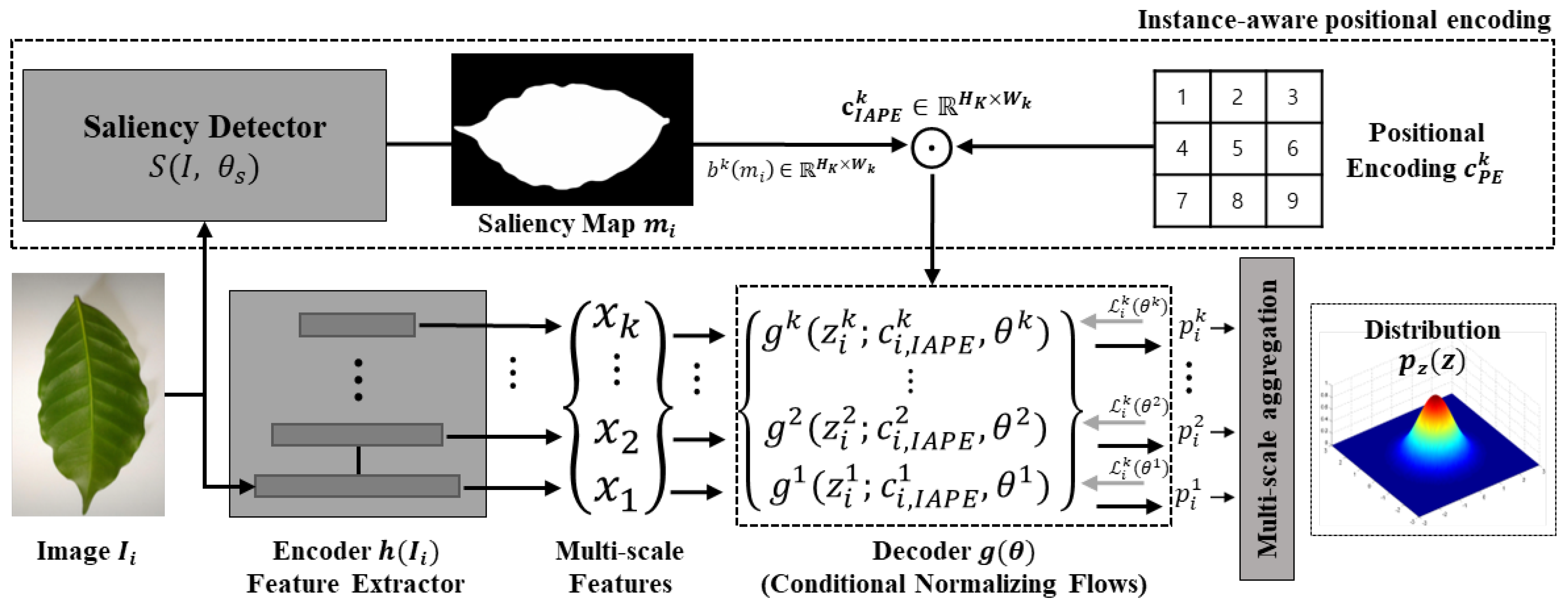
In the proposed pipeline shown in Figure 1, a CNN model is used as a feature extractor h to reduce the complexity of raw images and to extract meaningful features from them. Specifically, the feature extractor takes features from N layers in the CNN model; the N feature maps are used when constructing k multi-scale feature maps . Each layer in the CNN model has different structural and semantic properties, and the receptive field increases as the layer becomes deeper, which makes the model more capable of handling scale changes of diseased plants. Therefore, in this work, multi-scale features are used to robustly detect diseases on plants in real-world conditions.
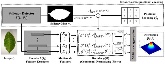
Figure 1.
Architecture of proposed approach IA-PDD. In this pipeline, RGB images are inputs to saliency detector and feature extractor . The saliency detector and feature extractor output a saliency map and multi-scale features, accordingly. Then, the saliency map, multi-scale features, and a positional encoding are fed into the set of decoders , a.k.a. conditional normalizing flows, independently. The outputs of the flow network are aggregated and then used to estimate multi-scale likelihoods . Finally, multi-scale likelihoods are used to calculate an anomaly score.
Most previous methods that used a CNN model as a feature extractor pre-trained the CNN model on ImageNet for generalized feature representation. However, due to the generalized characteristic learned from ImageNet, the pre-trained model tends to be too sensitive to semantic changes, such as leaf shadows and strong lighting, instead of focusing on diseased areas on plants. Therefore, the feature extractor needs to be re-trained to reduce the domain gap between generalized and specific domains, i.e., plant disease detection. However, pre-training the feature extractor in a supervised learning scheme requires labeled data, but the labeling process of plant diseases is hard due to shape changes of leaves and scarcity of images of diseased plants. Therefore, this work leverages self-supervised learning (SSL) to pre-train the feature extractor by using only unlabeled data , so that does not require any extra labeling process but uses only images of healthy plants and a few images of unhealthy plants.
3.3. Instance-Aware Positional Encoding
In this paper, we propose a method of instance-aware positional encoding (IAPE) using a visual saliency map—derived from the concept of human vision—as a visual attention map, which helps the proposed model to focus on plant leaves while casting aside background noise to efficiently detect diseased areas on unstructured plant leaves. The proposed approach, IAPE, can adaptively utilize spatial information of instances, which makes the model more aware of where the instances are located; this characteristic helps the model work robustly regardless of shape changes of plant leaves or background noise. The proposed method IAPE—instance-aware positional encoding—can be formulated as follows:
where S, , , and ⊙ refer to the saliency detector, visual saliency map, bilinear interpolation function, and elemental-wise product, respectively. denotes the combination of cos and sin terms used, to assign spatial information to the given feature map, a.k.a. sinusoidal positional encoding [41]. The saliency detector S receives input images and outputs the saliency map corresponding to the given image. Then is resized to the same resolution of each feature map from the proposed feature extractor by using a nearest-neighbor interpolation . In other words, the total number of resized should be equal to the number of feature maps taken from the feature extractor. Finally, the element-wise product ⊙ is applied between and the corresponding feature map, and the result is used as a conditional vector of the decoder in the proposed pipeline, to adaptively assign spatial information to the decoder and allow the proposed model to focus on where the instances are.
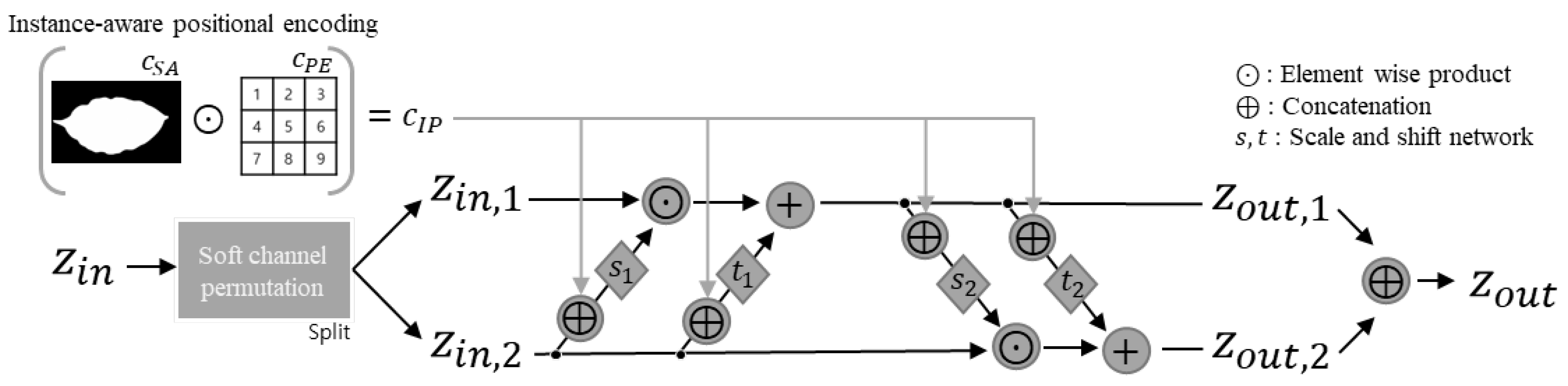
In addition, K independent decoders are used to estimate the density of multi-scale feature , which includes layer-specific information. The structures of these blocks are shown in Figure 2. The overall structure of g is basically a chain of blocks based on affine coupling layers [30]; g consists of three different operations, as follows: (1) soft-channel permutations [31]; (2) scaling; and (3) shifting. To apply scaling and shifting operations, the inputs are split into and using soft-channel permutations that adaptively generate permutations of the given inputs using a convolution layer. It then becomes a problem of multiplication and addition of subnetworks s and t, and this kind of operation is repeated. The shifting and scaling operations are defined as follows:
where ⊙ is the element-wise product. It is guaranteed that coefficients are always greater than 0 when applying a linear transformation (scaling), which preserves the affine properties. The internal functions s and t are differentiable functions, both of which are implemented in the fully connected and learnable network. The output and are concatenated, and the concatenated output is fed into a coupling layer . Furthermore, as is explained in Real-NVP [30], the logarithm of the Jacobian determinant for each matching block is simply defined as the summation of and . To train the proposed model, a maximum likelihood objective is employed, that is equivalent to minimizing the loss defined as follows:
where is the number of training samples. Furthermore, the random variable is equal to , and the Jacobian for the decoder of the proposed method. Detailed explanations of the loss are given in CFLOW-AD.
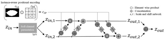
Figure 2.
Conditional affine coupling block with proposed instance-aware positional encoding.
4. Experiment and Results
4.1. Datasets
BRACOL (Weakly-unstructured). The BRACOL dataset has been mainly used for plant disease classification and segmentation of Arabica coffee leaves. The shapes of leaves are almost consistent, so we define this dataset as “weakly-unstructured”. The dataset consists of a total of 1747 images comprising 500 labeled data and 1247 unlabeled data. The labeled data include 100 images of healthy Arabica coffee leaves and 400 diseased leaves. The resolution of the original images is 1024 × 2048, which is scaled down to 256 × 256 using bilinear interpolation for the input size of the proposed model. In the labeled dataset, there are three classes, such as background, leaf, and symptom, where the symptom class is divided into 5 sub-classes: (1) Healthy; (2) Leaf miner; (3) Rust; (4) Brown leaf spot; and (5) Cercospora leaf spot. All images in the labeled dataset are manually pixel-level annotated, meaning that all pixels have their category labels, a.k.a. segmentation mask. The labeled dataset is used to test the performance of models, whereas the unlabeled dataset is used for pre-training the feature extractor.
PlantVillage (Unstructured). The PlantVillage dataset consists of a total of 54,303 images with 256 × 256 resolution, including 12 different types of crops. In this work, only 8 classes (tomatoes, apples, cherries, grapes, potatoes, peaches, peppers, strawberries) with both healthy and diseased leaves with corresponding labels are used. We exclude other classes due to the absence of the disease labels. We also randomly sample 100 images for each of the three cases, as follows: (1) normal training images; (2) normal test images; and (3) diseased test images. Therefore, a total of 2400 images is used for training and testing the proposed method, where the remaining group of images (i.e., 51,903 images) is used for self-supervised pre-training of the feature extractor.
4.2. Evaluation Metric
In this work, the image-level AUROC is used to evaluate the binary classification performance of models at an image-level, while pixel-level AUROC is used to evaluate the ability of models to localize diseased areas on plant leaves. For image-level AUROC, a single anomaly score and the ground truth class label of each test image are used. Likewise, in order to evaluate the performance of localizing anomalous areas on plant leaves at a pixel level, anomaly scores corresponding to each pixel are required. In other word, pixel-level AUROC enables a pixel-level evaluation using a binary ground truth mask for diseased areas on plant leaves and a score map of detection results. The pixel-level AUROC metric is only used for the BRACOL dataset, which contains ground truth labels for each pixel indicating whether the pixel is diseased or healthy. Predicted anomaly scores for each image or pixel are classified into four groups, such as true positive (TP), false positive (FP), true negative (TN), or false negative (FN), depending on whether they exceed a predetermined threshold and whether the predicted label matches the ground truth label. A true positive rate (TPR), indicating the sensitivity of models, and a false positive rate (FPR), indicating the specificity of models, can then be calculated as follows:
where TP, FP, FN, and TN refer to true positive, false positive, false negative, and true negative, respectively. Here, TPR and FPR are usually used as indicators of the sensitivity and specificity of models, respectively. However, taking only TPR and FPR into account may lead to unreliable results, as these values can change depending on the decision threshold. As a result, AUROC is selected as the metric for evaluation, as follows:
Since the evaluation metric, AUROC, is not only threshold-agnostic, but has also been employed in various other works, we used the same metric for all subsequent experiments.
4.3. Implementation Details
In this section, we explain the implementation details of the experiments from the feature extractor to the saliency detection network. All implementations and visualization are conducted in Pytorch and Anomallib [42] with a single NVIDIA DGX A100 GPU. For fair comparison and consistency, we used the same parameters for all experiments; the parameters mainly follow the same setting used in CFLOW-AD. First, as a feature extractor, we employ Wide-ResNet-50-2 [43] which, compared to ResNet [44], has a larger number of channels (by a factor of 2) for the bottleneck layer in every block. Then, the feature extractor is pre-trained on BRACOL and PlantVillage datasets in a self-supervised manner following the same learning strategy used in Simsiam [45]. During the pre-training process, the SGD optimizer is used with learning rate, weight decay, and 0.9 momentum where the batch size and epoch are set to 64 and 800, respectively. Second, during the training process, the pre-trained feature extractor is used to extract multi-scale features comprising features from layer2, layer3, and layer4, where the input images are resized to 224 × 224 by a bilinear interpolation. In addition, normal samples are used only for training and updating all learnable parameters except for the feature extractor, i.e., the freezing technique, whilst the evaluation dataset contains both normal and anomaly samples. Third, we leverage BASNet [46] pre-trained on the SOD [47] dataset to obtain a saliency map of mask-based feature encoding. All input images are resized to 256 × 256 and are used as inputs to estimate the saliency map. The saliency map is resized to be the same size as the multi-scale feature map; the resized saliency map is then used as a conditional vector of k decoders.
4.4. Experimental Results
To demonstrate the efficacy of the proposed approach, we compare the proposed model with state-of-the-art methods, such as PaDiM, PatchCore, and CFLOW-AD, on the BRACOL and PlantVillage datasets. These methods are all based on one-class classification which uses a single model for each class; the datasets have different characteristics. More specifically, the PlantVillage dataset includes more variable shape changes of leaves whereas the shapes of leaves in BRACOL are almost consistent. The evaluation is conducted at both image- and pixel-levels to observe the capability of detecting diseases and localizing areas of disease. To be precise, image-level plant disease detection aims to classify a given image into binary categories as follows: (1) Normal, when no disease appears in the image; and (2) Diseased, when the image contains any type of disease at the image-level. On the other hand, pixel-level plant disease detection aims to obtain corresponding categorical labels for every pixel, so that it can localize diseased areas on plants. Therefore, pixel-level plant disease detection is much more challenging but more useful in real-world conditions.
All tests are performed on two test datasets with distinct properties, as stated in Section 4.1 with respect to the AUROC evaluation metric. Specifically, shapes of plant leaves and viewpoints are nearly consistent on the BRACOL dataset (Weakly-unstructured), whereas they vary significantly on the PlantVillage dataset (Unstructured). First, as shown in Table 1, the performance differences between the proposed approach, IA-PDD, and the baseline model, CFLOW-AD, are only 0.10 and −0.34 at the image-level and pixel-level, respectively, on the weakly-unstructured BRACOL dataset. On the other hand, the proposed method outperforms CFLOW-AD by a large margin of 2.24 at the image-level on the unstructured PlantVillage dataset, as shown in Table 2. According to the results, there are variations in performance depending on the characteristics of the datasets used for evaluation. Specifically, it is demonstrated that the proposed model tends to have a higher performance on the unstructured dataset in which plant shapes and viewpoints vary significantly, whereas its performance on the weakly-unstructured dataset is only marginally different. The experimental result confirms that the combination of a saliency map, which is designed to simulate the human vision system, and positional encodings, which is designed to exploit spatial information in imagery, can improve the model’s performance in unstructured settings for plant disease detection.

Table 1.
Quantitative results for BRACOL [13] dataset at image- and pixel-levels with respect to AUROC, where “w/SSL” means “with self-supervised pretraining of feature extractor”.
Table 2.
Quantitative results for PlantVillage [14] dataset at image-level with respect to AUROC, where “w/SSL” means “with self-supervised pretraining of feature extractor”.
Plant disease detection models must be robust not only to the aforementioned issues, such as shape and viewpoint changes, but also to semantic noises, such as shadow and background changes. In this paper, we therefore propose the use of self-supervised learning (SSL) to pre-train the feature extractor without incurring any labeling cost in order to make the proposed model more robust to semantic noises and to improve the feature representation. After evaluation, it is determined that the performance of the proposed method achieves 99.96 and 99.99 at the image-level and pixel-level, respectively, with self-supervised pre-training, which is a 1.02 and 1.99 improvement over the performance without self-supervised pre-training, as shown in Table 1. Similarly, it is shown that the proposed model obtains a 98.25 image-level performance on the PlantVillage dataset with self-supervised pre-training, which is a 14.3 improvement over the performance without self-supervised pre-training, as shown in Table 2. In addition to the quantitative results, we also conducted qualitative analysis to confirm the validity and efficacy of the presented approaches.
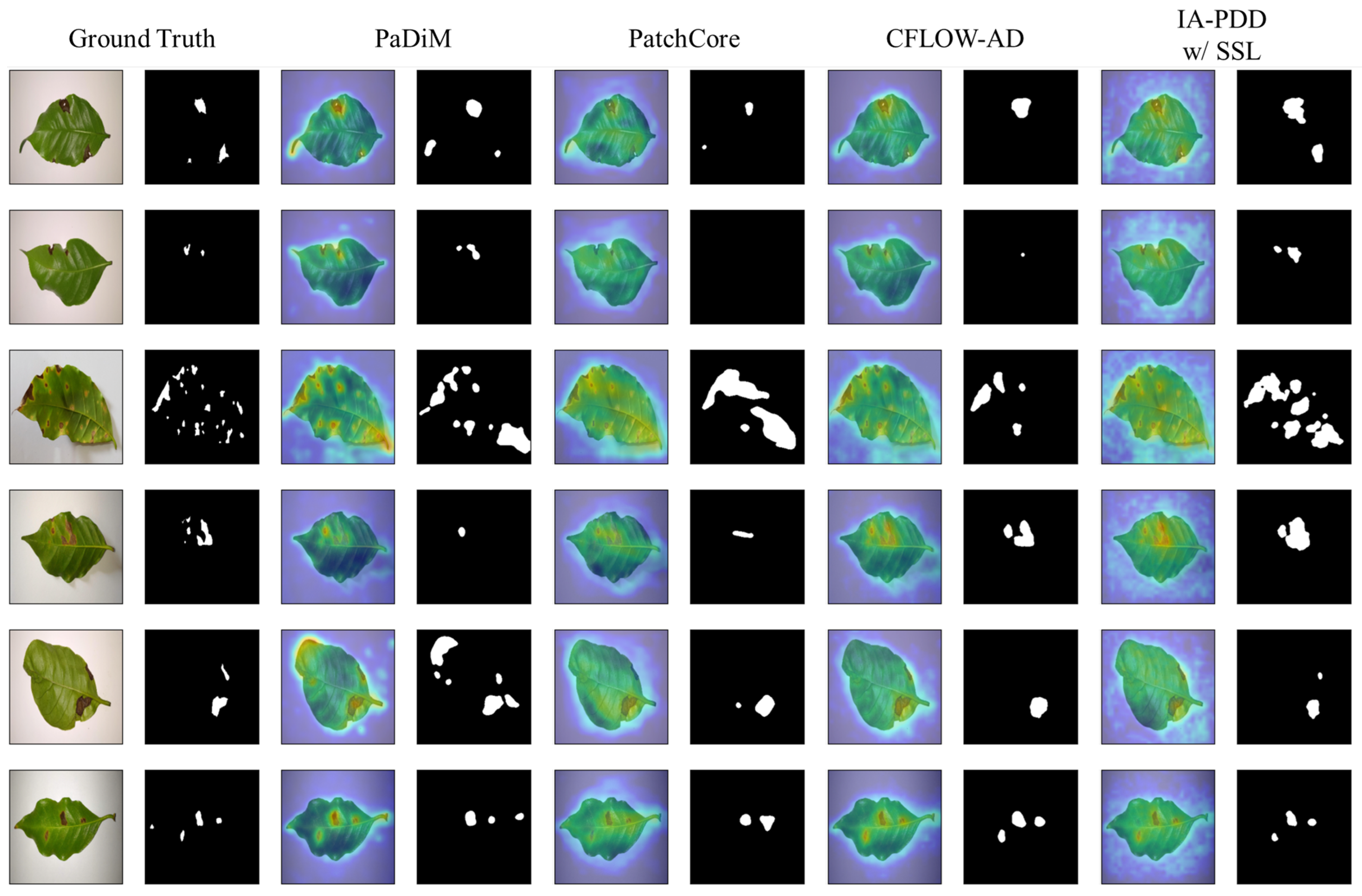
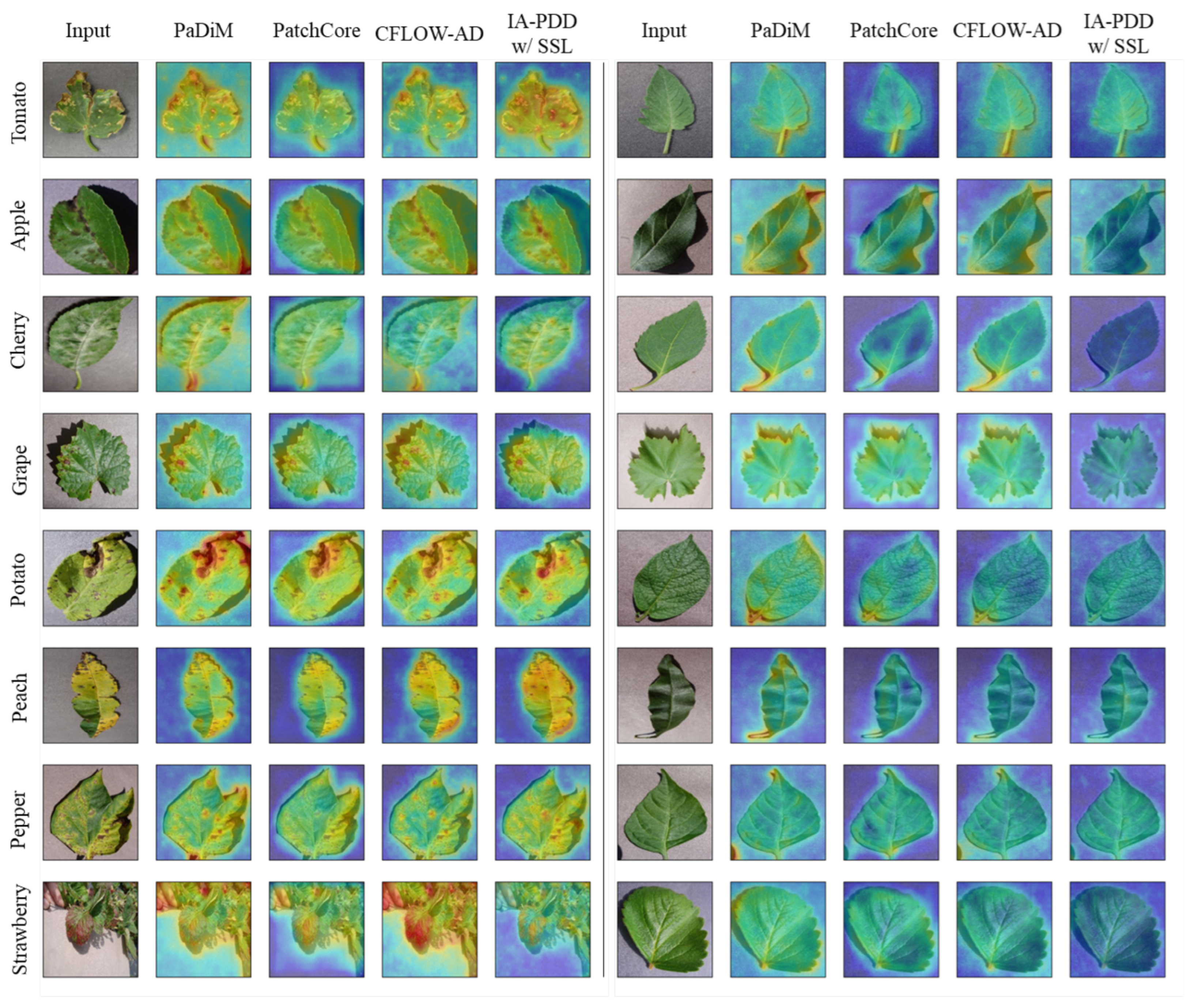
First, qualitative results on the BRACOL dataset demonstrate that the proposed model, IA-PDD, can identify tiny diseased areas that other models cannot detect when IAPE and SSL pre-training are used, as shown in Figure 3, the first and second rows. Second, the qualitative results of the PlantVillage dataset reveal a number of intriguing details. For instance, for particular classes of healthy leaves, such as tomato, cherry, potato, and peach, it is shown that the proposed model has generally lower uncertainty than other approaches, which tend to have high anomaly scores near pixels containing petioles with varying shapes. Moreover, for some classes, such as apple, grape, pepper, and strawberry, it is shown that the proposed approach continues to work robustly, but other methods incorrectly classify shadows as diseases. In addition, it is demonstrated that the proposed method obtains low anomaly scores for diseased plant leaves, such as apple, cherry, grape, and potato, whereas the other methods yield high anomaly scores near shadowing areas and petioles. Furthermore, it is proved that the proposed model can identify diseased areas even when they are ambiguous, whereas other models cannot perform well in certain cases in the figure, including apple, peach, and pepper. Lastly, in relation to the strawberry image in Figure 4, other methods tend to have high anomaly scores for background pixels but low anomaly scores for diseased pixels, whereas the proposed method works flawlessly.
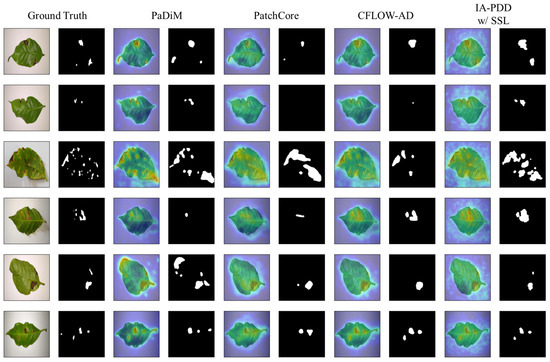
Figure 3.
Qualitative results on BRACOL dataset. The first two columns show input images and corresponding ground truth mask, respectively. The remaining group of columns represents the heat maps and corresponding predicted masks of the other state-of-the-art methods. In addition, each row shows qualitative results for randomly selected cases from the BRACOL dataset.
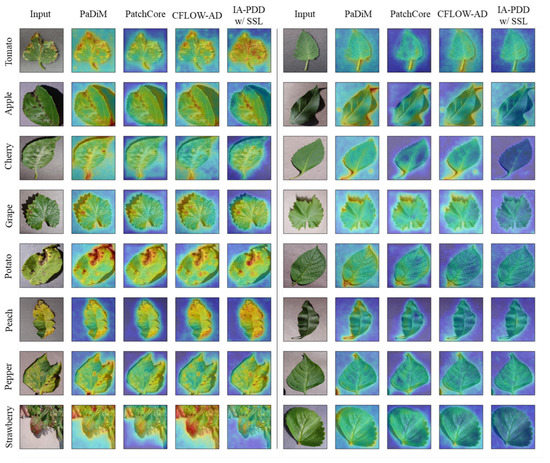
Figure 4.
Qualitative results on PlantVillage dataset. The first five columns show the results of diseased leaves; the remaining columns show results of healthy leaves. Unlike the BRACOL dataset, there are 8 class categories of plant leaves, and no ground truth mask exists in the PlantVillage dataset. Therefore, we provide only heat maps for each class (rows) in comparison with the other state-of-the-art methods (columns).
4.5. Ablation Study
Ablation studies were conducted to show how each component used in this work affects the others; this study was mainly divided into two parts: (1) performance difference depending on pre-training strategy of feature extractor; and (2) performance difference depending on structural changes in flow models. For consistency, we use the same backbone network Wide-ResNet-50-2 and 51,903 tomato images from PlantVillage, then compare the results with respect to image-level AUROC. The dataset is divided into training, test, and validation sets, with a ratio of 3:1:1. For supervised learning, the SGD optimizer is used with learning rate, weight decay, and 0.9 momentum where the batch size and epoch are set to 256 and 100, respectively.
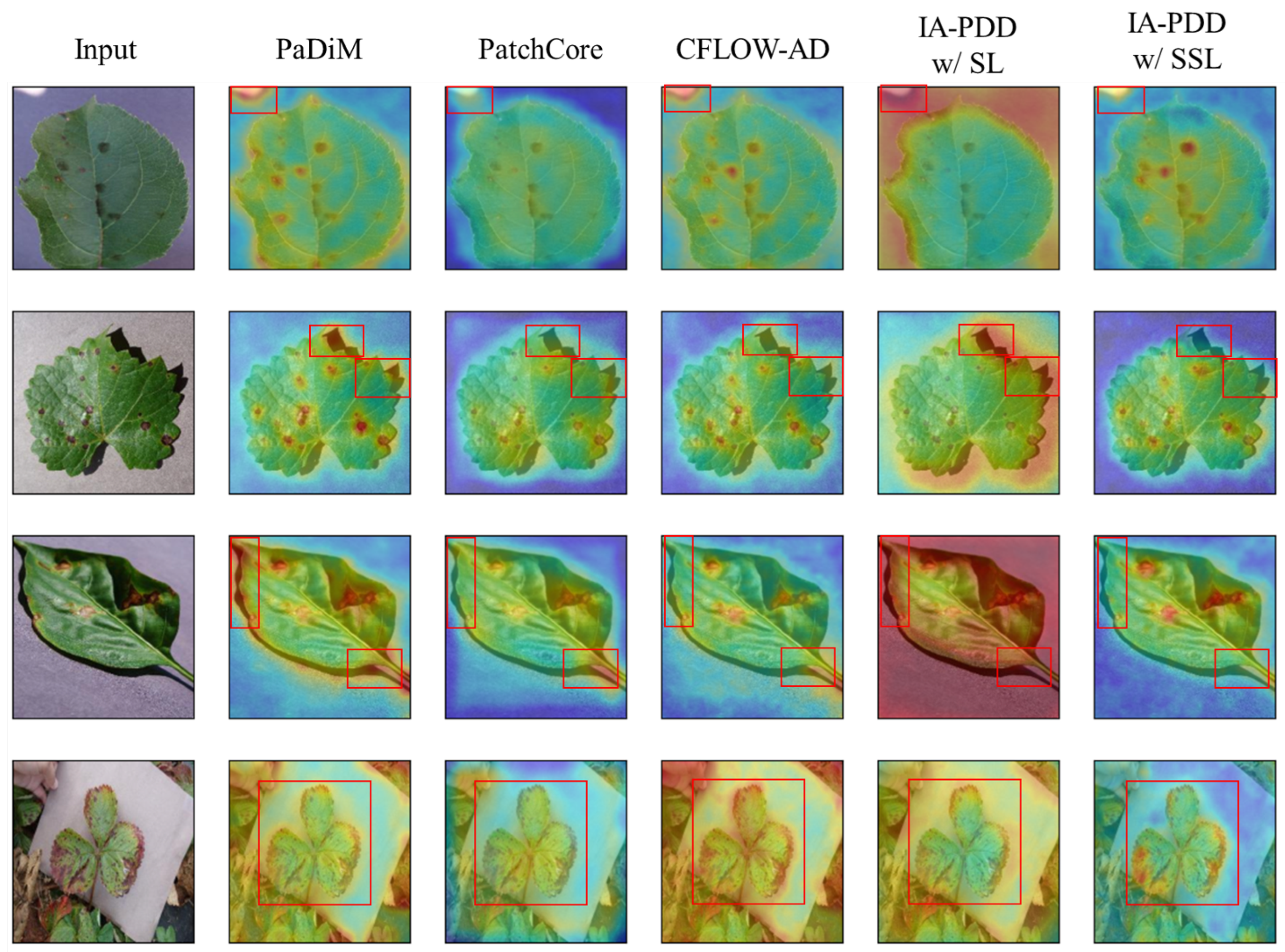
First, the experimental setup of the former case is subdivided into three categories to find the performance difference depending on the pre-training method of the feature extractor as follows: (1) supervised learning (SL) that uses labeled data; (2) ImageNet pretraining; (3) self-supervised learning (SSL) that only uses unlabeled data. It is shown that the average values of AUROC for each pre-training strategy achieved are 61.84, 80.23, and 94.55, respectively. Notably, a 28.95% performance increase is observed between SL and SSL, as shown in Figure 5. The qualitative result shown in Figure 5 also indicates that SSL is more capable than SL at detecting diseased areas on plant leaves. For example, the fifth column in the figure shows that SL tends to be too sensitive to semantic changes whereas the sixth column shows that SLL is not easily affected by background noise but only focuses on instances and diseased areas of those instances. Based on these results, it is verified that SSL achieves the best results in all cases.
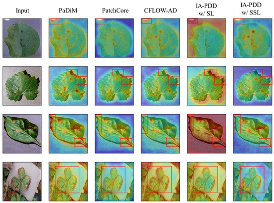
Figure 5.
Qualitative results of ablation study. The first two rows from the top are example cases of background noise; the two rows from the bottom correspond to example cases of unstructured data. We indicate areas where diseases are found with red boxes.
Second, the latter case is used to show performance differences depending on structural changes in decoders, i.e., flow models; results are summarized in Table 3. In the experiment, we increase the number of pooling layers from 2 to 4 where the number of conditional coupling layer blocks (# of CL) is set to 4 or 8. The average gain of each pretraining strategy between 4 and 8 CL blocks shows values of −1.95%, 3.4%, and 0.78%. From these results, it can be observed that more CL blocks usually guarantee better performance except for the SL case. SL shows the best performance of 67.44% AUROC with the 4-scale feature map and 4-coupling blocks (layer1, layer2, layer3, layer4). However, IA-PDD with ImageNet pretraining and SSL achieves the best performance values of 82.27% and 95.24% AUROC with 3-scale feature maps and 8 coupling blocks (layer2, layer3, layer4).
Table 3.
Results of ablation study. The ablation study was conducted to visualize performance differences depending on pre-training strategy of feature extractor and number of pooling layers (# of PL) and coupling layers (# of CL). SL, ImageNet, and SSL represent ways to pre-train the feature extractor; these are explained in Section 4.5.
5. Conclusions
In this work, we have introduced an instance-aware plant disease detector that can be used for plant disease detection. The proposed approach aims to effectively combine a visual saliency map and positional encodings to explicitly take spatial information into account. Specifically, the combined vectors are used as conditional vectors to normalizing flows and impart an instance-aware property. The combined vectors help the flow model to pay more attention to instances in which diseases are found and to reduce performance degradation caused by background noise. In addition, self-supervised learning is adopted for pre-training the feature extractor, which accounts for the robustness against semantic information changes of background and the strong feature representation. In our extensive plant disease detection experiments, it is shown that the proposed approach outperforms all one-class-classification-based state-of-the-art methods on commonly used datasets, such as BRACOL (Weakly-unstructured) and PlantVillage (Unstructured).
Author Contributions
Conceptualization, T.K. and Y.C.; methodology, T.K. and H.K.; software, T.K.; validation, T.K., and H.K.; formal analysis, T.K.; investigation, T.K. and H.K.; resources, K.B.; data curation, K.B.; writing—original draft preparation, T.K. and H.K.; writing—review and editing, T.K. and H.K.; visualization, T.K. and H.K.; supervision, Y.C.; project administration, Y.C.; funding acquisition, K.B. and Y.C. All authors have read and agreed to the published version of the manuscript.
Funding
This work was partly supported by the Institute of Information & Communications Technology Planning & Evaluation (IITP) grant funded by the Korea government (MSIT) (No. 2021-0-00755, 50%) and Korea Institute of Planning and Evaluation for Technology in Food, Agriculture and Forestry (IPET) and Korea Smart Farm R&D Foundation (KosFarm) through Smart Farm Innovation Technology Development Program, funded by Ministry of Agriculture, Food and Rural Affairs (MAFRA) and Ministry of Science and ICT (MSIT), Rural Development Administration (RDA) (No. 421033-04, 50%).
Institutional Review Board Statement
Not applicable.
Informed Consent Statement
Not applicable.
Data Availability Statement
Not applicable.
Conflicts of Interest
The authors declare no conflict of interest. The funders had no role in the design of the study; in the collection, analyses, or interpretation of data; in the writing of the manuscript, or in the decision to publish the results.
References
- Fry, W. Principles of Plant Disease Management; Academic Press: Cambridge, MA, USA, 1982. [Google Scholar]
- Zadoks, J.; Schein, R. Epidemiology and Plant Disease Management; Oxford University Press Inc: Oxford, UK, 1980. [Google Scholar]
- Worrall, E.; Hamid, A.; Mody, K.; Mitter, N.; Pappu, H. Nanotechnology for plant disease management. Agronomy 2018, 8, 285. [Google Scholar] [CrossRef]
- Khattab, A.; Habib, S.; Ismail, H.; Zayan, S.; Fahmy, Y.; Khairy, M. An IoT-based cognitive monitoring system for early plant disease forecast. Comput. Electron. Agric. 2019, 166, 105028. [Google Scholar] [CrossRef]
- Hwang, Y.; Lee, S.; Kim, T.; Baik, K.; Choi, Y. Crop Growth Monitoring System in Vertical Farms Based on Region-of-Interest Prediction. Agriculture 2022, 12, 656. [Google Scholar] [CrossRef]
- Shi, Y.; Wang, Z.; Wang, X.; Zhang, S. Internet of things application to monitoring plant disease and insect pests. In Proceedings of the 2015 International Conference on Applied Science Furthermore and Engineering Innovation, Jinan, China, 30–31 August 2015; pp. 31–34. [Google Scholar]
- Pavel, M.; Kamruzzaman, S.; Hasan, S.; Sabuj, S. An IoT based plant health monitoring system implementing image processing. In Proceedings of the 2019 IEEE 4th International Conference on Computer and Communication Systems (ICCCS), Singapore, 23–25 February 2019; pp. 299–303. [Google Scholar]
- Nagasubramanian, G.; Sakthivel, R.; Patan, R.; Sankayya, M.; Daneshmand, M.; Gandomi, A. Ensemble classification and IoT-based pattern recognition for crop disease monitoring system. IEEE Internet Things J. 2021, 8, 12847–12854. [Google Scholar] [CrossRef]
- Nandhini, M.; Kala, K.; Thangadarshini, M.; Verma, S. Deep Learning model of sequential image classifier for crop disease detection in plantain tree cultivation. Comput. Electron. Agric. 2022, 197, 106915. [Google Scholar] [CrossRef]
- Buja, I.; Sabella, E.; Monteduro, A.; Chiriacò, M.; De Bellis, L.; Luvisi, A.; Maruccio, G. Advances in plant disease detection and monitoring: From traditional assays to in-field diagnostics. Sensors 2021, 21, 2129. [Google Scholar] [CrossRef]
- Bedi, P.; Gole, P. Plant disease detection using hybrid model based on convolutional autoencoder and convolutional neural network. Artif. Intell. Agric. 2021, 5, 90–101. [Google Scholar] [CrossRef]
- Bhujel, A.; Kim, N.; Arulmozhi, E.; Basak, J.; Kim, H. A lightweight Attention-based convolutional neural networks for tomato leaf disease classification. Agriculture 2022, 12, 228. [Google Scholar] [CrossRef]
- Esgario, J.; Krohling, R.; Ventura, J. Deep learning for classification and severity estimation of coffee leaf biotic stress. Comput. Electron. Agric. 2020, 169, 105162. [Google Scholar] [CrossRef]
- Hughes, D.; Salathé, M. Others An open access repository of images on plant health to enable the development of mobile disease diagnostics. arXiv 2015, arXiv:1511.08060. [Google Scholar]
- Nazki, H.; Yoon, S.; Fuentes, A.; Park, D. Unsupervised image translation using adversarial networks for improved plant disease recognition. Comput. Electron. Agric. 2020, 168, 105117. [Google Scholar] [CrossRef]
- Benfenati, A.; Causin, P.; Oberti, R.; Stefanello, G. Unsupervised deep learning techniques for powdery mildew recognition based on multispectral imaging. arXiv 2021, arXiv:2112.11242. [Google Scholar]
- Zhang, S.; You, Z.; Wu, X. Plant disease leaf image segmentation based on superpixel clustering and EM algorithm. Neural Comput. Appl. 2019, 31, 1225–1232. [Google Scholar] [CrossRef]
- Douarre, C.; Crispim-Junior, C.; Gelibert, A.; Tougne, L.; Rousseau, D. Novel data augmentation strategies to boost supervised segmentation of plant disease. Comput. Electron. Agric. 2019, 165, 104967. [Google Scholar] [CrossRef]
- Gurrala, K.; Yemineni, L.; Rayana, K.; Vajja, L. A new segmentation method for plant disease diagnosis. In Proceedings of the 2019 2nd International Conference On Intelligent Communication Furthermore, Computational Techniques (ICCT), Jaipur, India, 28–29 September 2019; pp. 137–141. [Google Scholar]
- Buda, M.; Maki, A.; Mazurowski, M. A systematic study of the class imbalance problem in convolutional neural networks. Neural Netw. 2018, 106, 249–259. [Google Scholar] [CrossRef]
- Johnson, J.; Khoshgoftaar, T. Survey on deep learning with class imbalance. J. Big Data 2019, 6, 1–54. [Google Scholar] [CrossRef]
- Bergmann, P.; Fauser, M.; Sattlegger, D.; Steger, C. MVTec AD–A comprehensive real-world dataset for unsupervised anomaly detection. In Proceedings of the IEEE/CVF Conference on Computer Vision and Pattern Recognition, Long Beach, CA, USA, 15–20 June 2019; pp. 9592–9600. [Google Scholar]
- Defard, T.; Setkov, A.; Loesch, A.; Audigier, R. PaDiM: A patch distribution modeling framework for anomaly detection and localization. In International Conference on Pattern Recognition; Springer: Cham, Switzerland, 2021; pp. 475–489. [Google Scholar]
- Rudolph, M.; Wandt, B.; Rosenhahn, B. Same same but differnet: Semi-supervised defect detection with normalizing flows. In Proceedings of the IEEE/CVF Winter Conference on Applications of Computer Vision, Waikoloa, HI, USA, 3–8 January 2021; pp. 1907–1916. [Google Scholar]
- Gudovskiy, D.; Ishizaka, S.; Kozuka, K. Cflow-ad: Real-time unsupervised anomaly detection with localization via conditional normalizing flows. In Proceedings of the IEEE/CVF Winter Conference on Applications Of Computer Vision, Waikoloa, HI, USA, 3–8 January 2021; pp. 98–107. [Google Scholar]
- Rezende, D.; Mohamed, S. Variational inference with normalizing flows. In Proceedings of the 32nd International Conference on Machine Learning, ICML 2015, Lille, France, 6–11 July 2015; pp. 1530–1538. [Google Scholar]
- Goodfellow, I.; Pouget-Abadie, J.; Mirza, M.; Xu, B.; Warde-Farley, D.; Ozair, S.; Courville, A.; Bengio, Y. Generative Adversarial Networks. arXiv 2014, arXiv:1406.2661. [Google Scholar] [CrossRef]
- Bowman, S.; Vilnis, L.; Vinyals, O.; Dai, A.; Jozefowicz, R.; Bengio, S. Generating sentences from a continuous space. arXiv 2015, arXiv:1511.06349. [Google Scholar]
- Kingma, D.; Salimans, T.; Jozefowicz, R.; Chen, X.; Sutskever, I.; Welling, M. Improved Variational Inference with Inverse Autoregressive Flow. In Proceedings of the Advances In Neural Information Processing Systems, Barcelona, Spain, 5–10 December 2016; Volume 29. [Google Scholar]
- Dinh, L.; Sohl-Dickstein, J.; Bengio, S. Density estimation using real nvp. arXiv 2016, arXiv:1605.08803. [Google Scholar]
- Kingma, D.; Dhariwal, P. Glow: Generative flow with invertible 1x1 convolutions. In Proceedings of the Advances In Neural Information Processing Systems, Montreal, QC, Canada, 3–8 December 2018; Volume 31. [Google Scholar]
- Song, H.; Kim, M.; Park, D.; Shin, Y.; Lee, J. Learning from noisy labels with deep neural networks: A survey. IEEE Trans. Neural Netw. Learn. Syst. 2022, 1–19. [Google Scholar] [CrossRef]
- Roth, K.; Pemula, L.; Zepeda, J.; Schölkopf, B.; Brox, T.; Gehler, P. Towards total recall in industrial anomaly detection. arXiv 2021, arXiv:2106.08265. [Google Scholar]
- Kingma, D.; Welling, M. Auto-encoding variational bayes. arXiv 2013, arXiv:1312.6114. [Google Scholar]
- Yan, X.; Zhang, H.; Xu, X.; Hu, X.; Heng, P. Learning semantic context from normal samples for unsupervised anomaly detection. Proc. Aaai Conf. Artif. Intell. 2021, 35, 3110–3118. [Google Scholar]
- Dehaene, D.; Frigo, O.; Combrexelle, S.; Eline, P. Iterative energy-based projection on a normal data manifold for anomaly localization. arXiv 2020, arXiv:2002.03734. [Google Scholar]
- Hou, J.; Zhang, Y.; Zhong, Q.; Xie, D.; Pu, S.; Zhou, H. Divide-and-assemble: Learning block-wise memory for unsupervised anomaly detection. In Proceedings of the IEEE/CVF International Conference on Computer Vision, Montreal, QC, Canada, 10–17 October 2021; pp. 8791–8800. [Google Scholar]
- Katafuchi, R.; Tokunaga, T. Image-based Plant Disease Diagnosis with Unsupervised Anomaly Detection Based on Reconstructability of Colors. arXiv 2020, arXiv:2011.14306. [Google Scholar]
- Katafuchi, R.; Tokunaga, T. LEA-Net: Layer-wise External Attention Network for Efficient Color Anomaly Detection. arXiv 2021, arXiv:2109.05493. [Google Scholar]
- Kobyzev, I.; Prince, S.; Brubaker, M. Normalizing flows: An introduction and review of current methods. IEEE Trans. Pattern Anal. Mach. Intell. 2020, 43, 3964–3979. [Google Scholar] [CrossRef]
- Dosovitskiy, A.; Beyer, L.; Kolesnikov, A.; Weissenborn, D.; Zhai, X.; Unterthiner, T.; Dehghani, M.; Minderer, M.; Heigold, G.; Gelly, S.; et al. An image is worth 16 × 16 words: Transformers for image recognition at scale. In Proceedings of the 9th International Conference on Learning Representations, Vienna, Austria, 3–7 May 2021. [Google Scholar]
- Akçay, S.; Ameln, D.; Vaidya, A.; Lakshmanan, B.; Ahuja, N.; Genc, E. Anomalib: A Deep Learning Library for Anomaly Detection. arXiv 2022, arXiv:2202.08341. [Google Scholar]
- Zagoruyko, S.; Komodakis, N. Wide Residual Networks. arXiv 2016, arXiv:1605.07146. [Google Scholar]
- He, K.; Zhang, X.; Ren, S.; Sun, J. Deep residual learning for image recognition. In Proceedings of the IEEE Conference on Computer Vision and Pattern Recognition, Las Vegas, NV, USA, 27–30 June 2016; pp. 770–778. [Google Scholar]
- Chen, X.; He, K. Exploring simple siamese representation learning. In Proceedings of the IEEE/CVF Conference on Computer Vision and Pattern Recognition, Nashville, TN, USA, 19–25 June 2021; pp. 15750–15758. [Google Scholar]
- Qin, X.; Zhang, Z.; Huang, C.; Gao, C.; Dehghan, M.; Jagersand, M. Basnet: Boundary-aware salient object detection. In Proceedings of the IEEE/CVF Conference on Computer Vision and Pattern Recognition, Long Beach, CA, USA, 16–20 June 2019; pp. 7479–7489. [Google Scholar]
- Movahedi, V.; Elder, J. Design and perceptual validation of performance measures for salient object segmentation. In Proceedings of the 2010 IEEE Computer Society Conference on Computer Vision and Pattern Recognition-Workshops, San Francisco, CA, USA, 13–18 June 2010; pp. 49–56. [Google Scholar]
Publisher’s Note: MDPI stays neutral with regard to jurisdictional claims in published maps and institutional affiliations. |
© 2022 by the authors. Licensee MDPI, Basel, Switzerland. This article is an open access article distributed under the terms and conditions of the Creative Commons Attribution (CC BY) license (https://creativecommons.org/licenses/by/4.0/).