Abstract
In this study, three digital, site-specific, yield-mapping methods for winter wheat were examined, and their precision was evaluated. The crop yields of heterogeneous fields at three locations were determined on a site-specific basis using a yield-recording system composed of a combine harvester and algorithms based on reflection measurements made via satellites, as well as a tractor-mounted sensor. As a reference, the yield was determined with a plot harvester (ground truth data). The precision of the three methods was evaluated via statistical indicators (mean, median, minimum, maximum, and standard deviation) and correlation analyses between the yield of the ground truth data and the respective method. The results show a yield variation of 4.5–10.9 t ha−1 in the trial fields. The yield of the plot harvester was strongly correlated with the yield estimate from the sensor data (R2 = 0.71–0.75), it was moderately correlated with the yield estimate from the satellite data (R2 = 0.53–0.68), and it ranged from strongly to weakly correlated with the yield map of the combine harvester (R2 = 0.30–0.72). The absolute yield can be estimated using sensor data. Slight deviations (<10%) in the absolute yield are observed with the combine harvester, and there are clear deviations (±48%) when using the satellite data. The study shows differences in the precision and accuracy of the investigated methods. Further research and optimization are urgently needed to determine the exactness of the individual methods.
1. Introduction
Yield is the most important target criterion in crop production [1]. The crop yield determines the resource efficiency (nitrogen efficiency and energy efficiency) [2,3], environmental impact [4,5], and profitability of crop production [6,7]. The literature shows enormous differences in yields among fields in different soil and/or climatic areas around the world [8,9]. Various studies on the yield of winter wheat show a variation of 6.3 to 12.9 t ha−1 in southern Germany [5], 3.8 to 6.9 t ha−1 in eastern Germany [10], and 0.6 to 4.9 t ha−1 in the wheatbelt of Western Australia [11]. The crop yield depends on numerous overlapping influencing factors (genetic potential of the variety, fertilization, crop protection, and yield potentials of the soil and climate) [12,13,14]. The major reasons for these strong yield fluctuations are the differences in the yield potential of the soil, the topography, and the complex interactions with the climate and weather [15,16,17]. Soil properties such as soil texture, available water capacity, humus content, nutrient content, and pH vary at very small scales, leading to yield variations [5,18,19]. This results in small-scale fluctuating nutrient balances and nutrient stocks in soil, resulting in high emissions and nitrate losses in areas with low yield potential and overfertilization [5,20]. Nitrate loss into groundwater is a major problem [21]. Therefore, systems that are adapted to small-scale yield variations in crop management and fertilization will be required in the future. Site-specific land management, especially site-specific nitrogen fertilization, is promising [22,23,24,25]. This method can reduce the N surplus while increasing the N efficiency [4,5,26,27]. A prerequisite for the successful use of these digital methods is the delineation of management zones. Various parameters, such as yield maps (combine harvester data and hand sampling), biomass maps (satellite data), and soil parameters (available nitrogen, soil organic carbon, pH, available potassium, and bulk density), can be used to define the management zones of a field [28,29]. These parameters can be determined using different modern technologies such as multi- or hyperspectral measurements by sensors, drones or satellites, and georeferenced soil sampling.
Yield maps are one of the most important data sources for the delineation of management zones for site-specific fertilization; they can be supplemented with current crop measurements (e.g., nitrogen uptake with sensors or satellites) [1,30,31,32]. Recording the relative yield variability and absolute yield is important for precise site-specific fertilization [33]. A prerequisite for the development and use of yield maps is the availability of georeferenced yield data, which can be determined using various digital technologies [30,34,35]. Yield maps that are modeled based on these technologies may tend to over- or underestimate yield [36]. Additionally, there are various methods of filtering yield data based on the presence of outliers. Filter functions based on yield limits, moisture limits, travel distance, and yield surges are often used for this [37].
In this study, three different site-specific yield-mapping methods (sensor, satellite, and combine harvester) for winter wheat were investigated to evaluate their precision and suitability as a data basis for the delineation of yield and management zones for site-specific land management. For this purpose, plot trials were conducted in 2018, 2020, and 2021 at three different locations in southern Germany. The trials analyzed the precision of individual methods when mapping the harvested yield in the partial area, which is important to ensure the accuracy of the yield maps generated by these methods. The following aspects were investigated: (a) how accurately can the relative yield variation in the field be identified by the methods, and (b) how accurately can the methods estimate the absolute yield. In the trial plots, the yield was determined using a plot combine harvester (ground truth data) and digital georeferenced methods (sensor, satellite, and combine harvester). Correlation analyses that were determined using different methods evaluated the relationships among. Based on the results, the tested methods’ accuracy, precision, and suitability as the data basis for the delineation of management zones are evaluated.
2. Materials and Methods
2.1. Site and Weather Conditions
Three fields were selected for the study: in 2018, a field at the Dürnast Research Station (48°40′66″ N 11°69′49″ E), 3 km west of Freising (485 m a. s. l.), was selected, and in 2020 and 2021, experiments were conducted in two fields of the Makofen Research Farm (48°81′55″ N 12°74′31″ E), 15 km southeast of Straubing (320 m a. s. l.) (Figure 1).
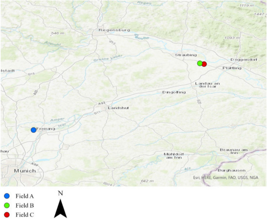
Figure 1.
Trial sites.
The trial field in Dürnast consists of medium-quality soil with hilly relief. The trial fields in Makofen are flat and characterized by very fertile loess soil. This classification is based on the soil fertility index [38]. Table 1 shows the most important soil parameters of the trial fields.

Table 1.
Soil data—Dürnast Research Station and Makofen.
An overview of temperature and precipitation at the trial sites is provided in Table 2. The 20-year mean annual precipitation is 789 mm, and the mean annual temperature is 8.7 °C at the Dürnast Research Station (Table 2). At the Makofen Research Farm, the 20-year mean annual precipitation is 781 mm, and the mean annual temperature is 9.5 °C (Table 2).
Table 2.
Mean temperature and precipitation—Dürnast Research Station and Makofen.
2.2. Crop Management
In 2018, the Reform winter wheat variety was grown on the trial field after grain corn. In 2020 and 2021, the Meister variety was grown on trial fields after sugar beet. In all trial years, the seedbed preparation was performed with plow and rotary harrow. Sowing, plant protection, and fertilization were uniformly conducted on the trial fields. Fertilization was conducted according to the fertilizer ordinance. Plant protection was conducted according to the infestation situation. Table 3 shows the crop management.
Table 3.
Crop management of the trial fields.
2.3. Experimental Design
The trial fields were divided into a grid of 15 m × 30 m plots. The outer 25 m of the trial fields were not included in the data analysis to avoid evaluating data from areas that did not belong to the field. This is important for methods based on satellite data in a 10 × 10 m grid to exclude measurement errors along the field edges [39]. The experimental setup was the same for all three experimental years, and only the number of plots differed (2018: n = 93; 2020: n = 106; 2021: n = 150) due to the different field sizes over the years. Figure 2 shows the experimental setup in 2020.
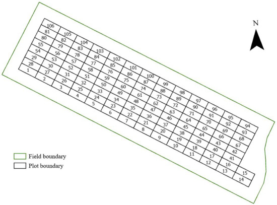
Figure 2.
Experimental setup (Field B, 2020).
2.4. Methods of Determining Yield
The wheat yield per plot was determined using the following methods:
- Plot harvester (ground truth data) [40];
- Combine harvester with yield mapping (mass flow sensor) [34];
- Process of Radiation, Mass, and Energy Transfer (PROMET) plant growth model based on satellite data (Sentinel-2) [41];
- Algorithm based on reflection measurements using a tractor-mounted multispectral sensor [42,43].
The winter wheat yield was determined with the plot harvester and the combine harvester with yield mapping (mass flow sensor) in the trial years on harvest dates of 27 July 2018, 30 July 2020, and 10 August 2021. A New Holland CX 8050 was used in 2018, and a John Deere S780 was used in 2020 and 2021 to map yields with a combine harvester. The PROMET estimate data were made available by the developer Vista GmbH. Depending on the availability, the PROMET plant growth model used satellite data shortly before the harvest date to estimate the yield [36]. Based on satellite data, the PROMET plant growth model calculated the yield considering further data [36]. The PROMET model requires four groups of model inputs that affect the spatial simulation of crop yield:
- Agricultural management (sowing date, fertilization events, harvest date);
- Crop specifications (variety, photoperiod sensitivity, assimilation rate);
- Dynamic environmental driver variables (temperature, precipitation, radiation, wind);
- Static environmental parameters (location, terrain, and soil properties) [36].
The reflection measurement for the algorithm by Maidl et al. [42] was conducted in the BBCH 65 growth stage. Based on this measurement, the REIP 700 vegetation index was calculated, and the algorithms used to estimate the yield were based on this index [42].
2.5. Data Processing
Considering the corresponding methodology, different digital methods were used to determine the yield for the entire field. Yield maps were generated based on point data. Next, these point data were visualized using geoinformation system software, ArcGIS [44], and assigned to the digitized plots via their coordinates. Data points on or outside the plot edges were eliminated. Depending on the method, the recorded yield data varied in terms of the spatial resolution and distribution in the plots. The plot combine harvester and combine harvester were driven immediately next to each other throughout the plot. Figure 3 shows the structure and data distribution of a plot in detail. The mean was calculated using all available yield values per plot. Thus, the yield per plot in t ha−1 was determined for each method for further analysis.
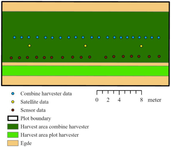
Figure 3.
Structure and data distribution in the plot.
2.6. Descriptive Statistics
The mean, median, minimum, maximum, and standard deviation were calculated for each method using R.
2.7. Correlation Analysis
Correlation analyses based on the yield per plot in t ha−1 determined the relationships between the yield values of the tested digital methods and the ground truth data. The coefficients of determination (R2) were classified as very strong (R2 > 0.9), strong (0.9 > R2 > 0.7), moderate (0.7 > R2 > 0.5), weak (0.5 > R2 > 0.3), or very weak (R2 < 0.3) [45].
3. Results
3.1. Spatial Variation in the Wheat Yield in 2018 (Field A)
Different site-specific yield mapping methods in 2018 led to different results for the yield distribution pattern, yield variation, and mean wheat yield in Field A (Figure 4, Table 4). The wheat yield, as determined by the plot harvester, varied between 6.1 and 10.9 t ha−1. The wheat yield measured by the mass flow sensor of the combine harvester (6.1–10.9 t ha−1) and the yield estimation made using algorithms based on sensor data (6.1–10.4 t ha−1) also varied, quite similarly to the ground truth data. The yield estimate made by the PROMET plant growth model based on satellite data (3.1–5.6 t ha−1) was also characterized by variability, but the yield variation of this method was not as great as those with the other methods, and a significantly lower yield level was noticeable (Figure 4). The mean wheat yield in field A, determined with the plot harvester, was 8.1 t ha−1, exactly corresponding to the sensor data yield; furthermore, when determined by the mass flow sensor of the combine harvester it was higher at 8.8 t ha−1 and when based on the satellite data it was lower at 4.2 t ha−1. This resulted in a deviation of +9% in the mean wheat yield of the combine harvester (mass flow sensor) and −48% when based on the satellite data compared to the ground truth data.
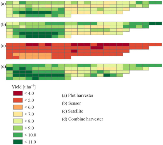
Figure 4.
Yield maps 2018, Field A. Yield determined from the plot harvester, sensor data, satellite data, and combine harvester.
Table 4.
Descriptive statistics of the yield data in t ha−1 analyzed in this study.
3.2. Spatial Variation in the Wheat Yield in 2020 (Field B)
The yields in 2020, determined using different digital methods, led to similar overall results. In contrast to 2018, the yield variability was significantly lower in 2020 (Figure 5, Table 4). The yield variation based on satellite data (8.3–10.1 t ha−1) and determined by the mass flow sensor of the combine harvester (8.4–10.2 t ha−1) corresponded to the ground truth data (8.4–10.1 t ha−1). The yield estimate based on the sensor data showed a slightly higher yield variability (6.8–10.4 t ha−1). However, the yield distribution pattern matched the ground truth data well (Figure 5). The mean wheat yield of the ground truth data for field B was 9.3 t ha−1 and corresponded with the yields based on the sensor and satellite data, while that determined by the mass flow sensor of the combine harvester (9.8 t ha −1) was slightly higher. Overall, the deviations in the mean wheat yields were small (<5%).
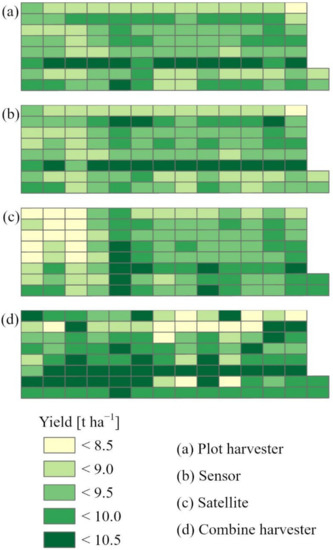
Figure 5.
Yield maps 2020, Field B. Yield determined from the plot harvester, sensor data, satellite data, and combine harvester.
3.3. Spatial Variation in the Wheat Yield in 2021 (Field C)
In 2021, there were differences in the results of various digital methods (Figure 6, Table 4). As in 2018, the yields determined using satellite data with the PROMET model clearly differed from the results of the other yield-mapping systems. However, the yields based on the satellite data were much higher in 2021 and much lower than the results of the other measurement systems in 2018 (Figure 4 and Figure 6). The yields of the combine harvester (3.7–7.8 t ha−1) and the sensor data (4.4–7.2 t ha−1) were very similar to the ground truth data (4.5–7.5 t ha−1) in terms of yield variation and distribution pattern. The yield estimate based on the satellite data (7.2–9.6 t ha−1) showed less yield variation at a significantly higher yield level (Figure 6), resulting in a deviation of +44% in the mean wheat yield of the satellite data (8.5 t ha−1) compared to the ground truth data (5.9 t ha−1) in field C. The mean wheat yields of the combine harvester and sensor data corresponded to the ground truth data.
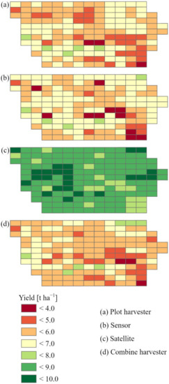
Figure 6.
Yield maps 2021, Field C. Yield determined from the plot harvester, sensor data, satellite data, and combine harvester.
3.4. Correlation between Variables
Table 5 shows the coefficients of determination (R2) of the linear and polynomial relationships (second degree) of the wheat yields, determined using various digital methods.
Table 5.
Coefficients of determination (R2): yield data for 2018 (n = 93), 2020 (n = 106), and 2021 (n = 150).
3.4.1. Field A (2018)
In 2018, the correlation analysis showed a strong relationship between the ground truth data and the yield estimate from the sensor data (R2 = 0.75). The yield estimate from the satellite data (R2 = 0.68) and the yield map from the combine harvester (R2 = 0.69) were moderately correlated with the ground truth data.
3.4.2. Field B (2020)
In 2020, the correlations between the yield data of the tested methods were very different. As in the previous year, there was a strong relationship between the ground truth data and the yield estimate based on sensor data (R2 = 0.71). The yield estimates from the satellite data and ground truth data showed a moderate correlation (R2 = 0.53), while that from the combine harvester only weakly correlated with the ground truth data (R2 = 0.30) (Table 5).
3.4.3. Field C (2021)
In 2021, all the methods resulted in moderate or strong relationships. Strong correlations were determined between the ground truth data and the yield data from the combine harvester (R2 = 0.72) as well as the sensor data (R2 = 0.71). The correlation between the ground truth data and the estimate from the satellite data (R2 = 0.56) was moderate (Figure 7 and Table 5).
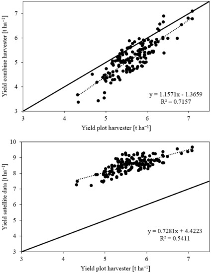
Figure 7.
The linear relationships between the yields of ground truth data (plot harvester) and combine harvester (above) as well as satellite data (below) in field C in 2021.
4. Discussion
4.1. Discussion of the Methods
In this study, three different site-specific yield-mapping methods for winter wheat were tested on heterogeneous fields at three locations in southern Germany. The precision of the methods was tested by comparing the statistical indicators (mean, median, minimum, maximum, and standard deviation), mapping the yield distribution patterns and investigating the correlative relationships. The aim was to identify the yield distribution patterns and analyze the absolute wheat yields.
4.1.1. Site Selection
The yield variability results were particularly influenced by the heterogeneity of the trial fields [46,47]. In homogeneous fields, a lower yield variation was expected; therefore, these fields were not suitable for a comparison of the methods [5,48]. As a result, heterogeneous fields were selected for this investigation. The heterogeneity was assessed based on soil properties, biomass maps, and the expertise of the farm managers. The expertise of the farm managers was a suitable basis for assessing the heterogeneity of a field [49]. Furthermore, the literature shows that small-scale variations in the soil parameters and yield are characteristic of the study region [50].
4.1.2. Ground Truth Data
The yield data were determined using various digital methods. Suitable ground truth data (yield measurements) were crucial in evaluating the various digital yield-mapping methods so that the modeled data could be compared with the measured data [5]. Therefore, in this study, all plots were harvested by a plot harvester with a weighing system [40]. The plot harvester facilitated the determination of the correct wheat yield per plot and the evaluation of the yield maps determined using digital methods. The plot harvester and combine harvester could not harvest the same area, resulting in minor deviations in their measured values. They drove next to each other through the plots. However, the variance in the difference decreases with the distance between two measurement points, which is the basis for the geostatistical methods (kriging interpolation) used in many studies on yield variability [5,51,52,53]. Therefore, this approach provided ground truth data with very high measurement accuracy.
Since the use of a plot harvester is labor-intensive and can hardly be implemented for large fields, similar studies compared the modeled yield data with the yield map data from a combine harvester [1,32,54]. However, this requires high precision when mapping yields with a combine harvester. Investigations showed considerable uncertainties in mapping yields using a combine harvester due to various error sources. Sensor errors, operating errors, errors due to operating conditions, and data processing were the most common causes of uncertainty [34,55,56]. In particular, constantly changing operating conditions during harvest, different measurement systems, and principles for combine harvesters from different manufacturers and, sometimes, missing or inaccurate calibration led to uncertainties in the combine harvester data [57,58,59]. Despite further development of the yield-mapping systems in combine harvesters, the fluctuation in the correlations between the ground truth data and the combine harvester data from R2 = 0.30 to 0.72 showed clear differences in the precision of the combine harvester data in this study. In a study by Hülsbergen et al. [60], the combine harvester data from individual fields were strongly correlated with ground truth data (plot harvester and biomass samples), while this correlation was weak in other fields. Therefore, the ground truth data from the plot harvester were of immense importance to the evaluation of various methods in this study. Alternatively, georeferenced biomass samples can also provide ground truth data. However, the measurement effort is a limiting factor. Mittermayer et al. [5] collected 50 biomass samples in a 13.1 ha area in his investigations, determined the yield with a laboratory thresher, and conducted data analysis using geostatistical methods.
4.2. Discussion of the Results
The yield variation in the three trial years (2018: 6.1 to 10.9 t ha−1, 2020: 8.4 to 10.1 t ha−1, and 2021: 4.5 to 7.5 t ha−1) was clear. By analyzing several fields and research years, the optimal conditions to evaluate the precision of various digital yield-mapping methods were given. Several scientific studies addressed the mapping of the yield variability of winter wheat, but most of these studies only used one method [10,23,32,36,52]. Only a few studies compared ground truth data with data from different digital systems.
4.2.1. Sensor Data
The yield estimate based on multispectral sensor data, the REIP vegetation index, and a crop-specific yield algorithm [42] provided high-precision yield maps in all three years (2018: R2 = 0.75, 2020: R2 = 0.71, and 2021: R2 = 0.71). In addition, this method showed only minor deviations in the yield variation and the mean wheat yield of max. ±1%. Hauser et al. [10] also compared plot harvester data with sensor data and achieved similar results (R2 = 0.70). Kaivosoja et al. [54] compared sensor data with combine harvester data and found a strong correlation (R2 = 0.82). These results confirm the potential of continuously generating very precise yield data from sensor data. The prerequisites for obtaining high yield-mapping accuracy using this method are multispectral sensors with high measurement accuracy, suitable vegetation indices, and scientific-based yield algorithms [42,61,62].
4.2.2. Combine Harvester
The yield data of the combine harvester (mass flow sensor) provided yield maps of at least moderate or good quality in 2018 and 2021 (2018: R2 = 0.69 and 2021: R2 = 0.72). In 2020, however, the combine harvester data were only weakly correlated with the ground truth data (R2 = 0.30). A maximum deviation in the yield variation and the mean wheat yield of ±9% showed that the bad correlation in 2020 was mainly due to an incorrect mapping of the yield distribution pattern. A New Holland combine harvester was used in 2018, while a John Deere combine harvester was used in 2020 and 2021. All three combine harvesters determined the yield using a mass flow sensor. However, the John Deere combine was equipped with “active yield” in 2021, which means that the mass flow sensor in the grain elevator was continuously calibrated using load cells installed in the grain tank [63]. This possibly led to a considerable improvement in the precision of the combine harvester data between 2020 and 2021, as all other conditions (driver, calibration, model, working width, etc.) were identical for both years. These results confirmed the conclusions of previous studies of the uncertainties in combine harvester data [34,55,56,57]. The central causes of uncertainties, such as calibration and automatic cutting width detection, can be improved through further developments by the manufacturer. Operating errors can be avoided through intensive driver training. Varying environmental influences and operating conditions, such as different material moisture levels, soiling of the sensors by crop residues, abrupt changes in speed, or grain plants lying on the ground will limit the accuracy of combine harvester data in the future [58,59]. However, the strong correlations in some cases show the combine harvesters’ potential for mapping yields and their spatial variability.
4.2.3. Satellite Data
The yield maps of the PROMET plant growth model, based on satellite data, depict the yield distribution pattern moderately in all three years (2018: R2 = 0.68, 2020: R2 = 0.53, and 2021 R2 = 0.56). The method achieved a maximum deviation of ±48% in the yield variation and the mean wheat yield. Since the relative yield distribution pattern was identified at least moderately in all three trial years, these significant deviations resulted from underestimating (2018) and overestimating (2021) the absolute yield. In both years, weather extremes were observed. In 2018, the weather was hotter and drier than average; in 2021, the weather was colder and wetter than average. In addition to satellite data, the PROMET plant growth model requires various groups of model inputs that affect the spatial simulation of plant development, such as agricultural management (sowing date, fertilization events, harvest date, etc.), crop specifications (variety, photoperiod sensitivity, assimilation rate, etc.), dynamic environmental driver variables (temperature, precipitation, radiation, wind, etc.), and static environmental parameters (location, terrain, and soil properties) [36]. The model may react too strongly to weather data, which means that the model can no longer model reliable absolute yield data in years with extreme meteorological conditions. In this context, Hank et al. [36] also found tendencies to overestimate yields in extreme weather conditions. However, further studies are necessary to assess this assumption and the precision of satellite data-based methods in more detail [5,24,64]. Hank et al. [36] also compared the modeled yield data of the PROMET plant growth model with combine harvester data, finding a strong correlation (R2 = 0.82). Toscano et al. [59] correlated Sentinel 2 and Landsat 8 satellite data with yield data from hand samples and combine harvesters and found correlations varying from moderate to strong (R2 = 0.54–0.74). Zhao et al. [32] also compared Sentinel 2 satellite data with combine harvester data and found a stronger correlation (R2 = 0.76). These results confirm the potential to derive yield zones with satellite data. However, the absolute yield can deviate for data modeled with PROMET based on satellite data, leading to crop management problems. For example, in the case of yield maps for fertilization, the absolute yield is important; otherwise, the crop would be fertilized incorrectly. Therefore, further investigations are urgently needed to reduce deviations, such as those conducted in 2018 and 2021.
5. Conclusions
Yield maps are one of the most important sources of data for the delineation of management zones for site-specific land management. Therefore, precise yield maps are required to derive high-quality management zones. The results of this study show that the yield maps from the sensor data are best suited to delineate management zones. The yield maps of the combine harvester in 2018 and 2021 are also quite suitable, unlike those from 2020. This can lead to faulty management zones. Incorrect management zones result in inefficient crop management, thus causing environmental pollution. Therefore, further investigations are needed to optimize and develop yield-mapping systems for combine harvesters. The aim should be to generate yield maps with consistent quality, using modern combine harvesters to collect high-quality data easily and inexpensively during harvest. The results of the satellite data depict the relative yield distribution patterns as being moderate over all trial years and are, therefore, suitable for the creation of relative biomass maps. However, due to the deviations in the absolute yields, these results are only suitable for yield potential maps to a limited extent, and further research is required to improve the results. Overall, each method shows enormous potential to generate yield maps. Nevertheless, there are individual problems that urgently need further investigation to improve the precision of all methods.
Author Contributions
Conceptualization, M.S. and F.-X.M.; methodology, M.S. and F.-X.M.; investigation, M.S. and M.M.; data curation, M.S. and M.M.; writing—original draft preparation, M.S.; writing—review and editing, M.M., F.-X.M., K.-J.H. and H.B.; project administration, J.S.; funding acquisition, J.S. All authors have read and agreed to the published version of the manuscript.
Funding
This research was funded by the European Commission and the State of Bavaria as part of EIP-Agri (EP4-904).
Institutional Review Board Statement
Not applicable.
Informed Consent Statement
Not applicable.
Data Availability Statement
The data presented in this study are available from the corresponding author upon reasonable request.
Acknowledgments
We would like to thank VISTA Geowissenschaftliche Fernerkundung GmbH (Gabelsbergerstraße 51, 80333 Munich, Germany) for providing yield maps using satellite data and a crop growth model.
Conflicts of Interest
The authors declare no conflict of interest.
References
- Hunt, M.L.; Blackburn, G.A.; Carrasco, L.; Redhead, J.W.; Rowland, C.S. High resolution wheat yield mapping using Sentinel-2. Remote Sens. Environ. 2019, 233, 111410. [Google Scholar] [CrossRef]
- Barraclough, P.B.; Howarth, J.R.; Jones, J.; Lopez-Bellido, R.; Parmar, S.; Shepherd, C.E.; Hawkesford, M.J. Nitrogen efficiency of wheat: Genotypic and environmental variation and prospects for improvement. Eur. J. Agron. 2010, 33, 1–11. [Google Scholar] [CrossRef]
- Duan, J.; Shao, Y.; He, L.; Li, X.; Hou, G.; Li, S.; Feng, W.; Zhu, Y.; Wang, Y.; Xie, Y. Optimizing nitrogen management to achieve high yield, high nitrogen efficiency and low nitrogen emission in winter wheat. Sci. Total Environ. 2019, 697, 134088. [Google Scholar] [CrossRef]
- Cui, Z.; Zhang, F.; Chen, X.; Dou, Z.; Li, J. In-season nitrogen management strategy for winter wheat: Maximizing yields, minimizing environmental impact in an over-fertilization context. Field Crops Res. 2010, 116, 140–146. [Google Scholar] [CrossRef]
- Mittermayer, M.; Gilg, A.; Maidl, F.X.; Nätscher, L.; Hülsbergen, K.J. Site-specific nitrogen balances based on spatially variable soil and plant properties. Precis. Agric. 2021, 22, 1416–1436. [Google Scholar] [CrossRef]
- Fan, R.; Zhang, X.; Liang, A.; Shi, X.; Chen, X.; Bao, K.; Yang, X.; Jia, S. Tillage and rotation effects on crop yield and profitability on a Black soil in northeast China. Can. J. Soil Sci. 2012, 92, 463–470. [Google Scholar] [CrossRef]
- Klima, K.; Kliszcz, A.; Puła, J.; Lepiarczyk, A. Yield and profitability of crop production in mountain less favoured areas. Agronomy 2020, 10, 700. [Google Scholar] [CrossRef]
- Hakojärvi, M.; Hautala, M.; Ristolainen, A.; Alakukku, L. Yield variation of spring cereals in relation to selected soil physical properties on three clay soil fields. Eur. J. Agron. 2013, 49, 1–11. [Google Scholar] [CrossRef]
- Zebarth, B.J.; Fillmore, S.; Watts, S.; Barrett, R.; Comeau, L.P. Soil factors related to within-field yield variation in commercial potato fields in Prince Edward Island Canada. Am. J. Potato Res. 2021, 98, 139–148. [Google Scholar] [CrossRef]
- Hauser, J.; Maidl, F.X.; Wagner, P. Untersuchung der teilflächenspezifischen Ertragserfassung von Großmähdreschern in Winterweizen (Investigation of site-specific yield mapping of combine harvesters in winter wheat). In Proceedings of the 41st GIL-Jahrestagung, Potsdam, Germany, 8–9 March 2021; pp. 133–138. [Google Scholar]
- Robertson, M.J.; Lyle, G.; Bowden, J.W. Within-field variability of wheat yield and economic implications for spatially variable nutrient management. Field Crops Res. 2008, 105, 211–220. [Google Scholar] [CrossRef]
- Bertic, B.; Loncaric, Z.; Vukadinovic, V.; Vukobratovic, Z.; Vukadinovic, V. Winter wheat yield responses to mineral fertilization. Cereal Res. Commun. 2007, 35, 245–248. [Google Scholar] [CrossRef]
- Cabas, J.; Weersink, A.; Olale, E. Crop yield response to economic, site and climatic variables. Clim. Chang. 2009, 101, 599–616. [Google Scholar] [CrossRef]
- Fasoula, V.A.; Fasoula, D.A. Principles underlying genetic improvement for high and stable crop yield potential. Field Crops Res. 2002, 75, 191–209. [Google Scholar] [CrossRef]
- Buttafuoco, G.; Castrignanò, A.; Colecchia, A.S.; Ricca, N. Delineation of management zones using soil properties and a multivariate geostatistical approach. Ital. J. Agron. 2010, 5, 323–332. [Google Scholar] [CrossRef]
- Farid, H.U.; Bakhsh, A.; Ahmad, N.; Ahmad, A.; Mahmood-Khan, Z. Delineating site-specific management zones for precision agriculture. J. Agric. Sci. 2016, 154, 273–286. [Google Scholar] [CrossRef]
- Moral, F.J.; Terrón, J.M.; Rebollo, F.J. Site-specific management zones based on the Rasch model and geostatistical techniques. Comput. Electron. Agric. 2011, 75, 223–230. [Google Scholar] [CrossRef]
- López-Lozano, R.; Casterad, M.A.; Herrero, J. Site-specific management units in a commercial maize plot delineated using very high resolution remote sensing and soil properties mapping. Comput. Electron. Agric. 2010, 73, 219–229. [Google Scholar] [CrossRef]
- Servadio, P.; Bergonzoli, S.; Verotti, M. Delineation of management zones based on soil mechanical-chemical properties to apply variable rates of inputs throughout a field (VRA). Eng. Agric. Environ. 2017, 10, 20–30. [Google Scholar] [CrossRef]
- Dalgaard, T.; Bienkowski, J.F.; Bleeker, A.; Dragosits, U.; Drouet, J.L.; Durand, P.; Frumau, A.; Hutchings, N.J.; Kedziora, A.; Magliulo, V.; et al. Farm nitrogen balances in six European landscapes as an indicator for nitrogen losses and basis for improved management. Biogeosciences 2012, 9, 5303–5321. [Google Scholar] [CrossRef]
- Strebel, O.; Duynisveld, W.H.M.; Böttcher, J. Nitrate pollution of groundwater in western Europe. Agric. Ecosyst. Environ. 1989, 26, 189–214. [Google Scholar] [CrossRef]
- Diacono, M.; Rubino, P.; Montemurro, F. Precision nitrogen management of wheat. A review. Agron. Sustain. Dev. 2013, 33, 219–241. [Google Scholar] [CrossRef]
- Liu, H.; Whiting, M.L.; Ustin, S.L.; Zarco-Tejada, P.J.; Huffman, T.; Zhang, X. Maximizing the relationship of yield to site-specific management zones with object-oriented segmentation of hyperspectral images. Precis. Agric. 2018, 19, 348–364. [Google Scholar] [CrossRef]
- Mulla, D.J. Twenty five years of remote sensing in precision agriculture: Key advances and remaining knowledge gaps. Biosyst. Eng. 2013, 114, 358–371. [Google Scholar] [CrossRef]
- Prücklmaier, J. Feldexperimentelle Analysen zur Ertragsbildung und Stickstoffeffizienz bei Organisch-Mineralischer Düngung auf Heterogenen Standorten und Möglichkeiten zur Effizienzsteigerung durch Computer- und Sensorgestützte Düngesysteme (Field Experimental Analyses of Yield Effects and Nitrogen Efficiency of Fertilizer Application Systems). Ph.D. Thesis, Technische Universität München, Munich, Germany, 2020. [Google Scholar]
- Argento, F.; Anken, T.; Abt, F.; Vogelsanger, E.; Walter, A.; Liebisch, F. Site-specific nitrogen management in winter wheat supported by low-altitude remote sensing and soil data. Precis. Agric. 2020, 22, 364–386. [Google Scholar] [CrossRef]
- Vinzent, B.; Fuß, R.; Maidl, F.X.; Hülsbergen, K.J. Efficacy of agronomic strategies for mitigation of after-harvest N2O emissions of winter oilseed rape. Eur. J. Agron. 2017, 89, 88–96. [Google Scholar] [CrossRef]
- Brock, A.; Brouder, S.M.; Blumhoff, G.; Hofmann, B.S. Defining yield-based management zones for corn-soybean rotations. Agron. J. 2005, 97, 1115–1128. [Google Scholar] [CrossRef]
- Yao, R.J.; Yang, J.S.; Zhang, T.J.; Gao, P.; Wang, X.P.; Hong, L.Z.; Wang, M.W. Determination of site-specific management zones using soil physico-chemical properties and crop yields in coastal reclaimed farmland. Geoderma 2014, 232, 381–393. [Google Scholar] [CrossRef]
- Blasch, G.; Li, Z.; Taylor, J.A. Multi-temporal yield pattern analysis method for deriving yield zones in crop production systems. Precis. Agric. 2020, 21, 1263–1290. [Google Scholar] [CrossRef]
- Jin, Z.; Azzari, G.; Lobell, D.B. Improving the accuracy of satellite-based high-resolution yield estimation: A test of multiple scalable approaches. Agric. For. Meteorol. 2017, 247, 207–220. [Google Scholar] [CrossRef]
- Zhao, Y.; Potgieter, A.B.; Zhang, M.; Wu, B.; Hammer, G.L. Predicting wheat yield at the field scale by combining high-resolution Sentinel-2 satellite imagery and crop modelling. Remote Sens. 2020, 12, 1024. [Google Scholar] [CrossRef]
- Maidl, F.X.; Schächtl, J.; Huber, G. Strategies for site-specific nitrogen fertilization on winter wheat. In Proceedings of the 7th International Conference on Precision Agriculture and other Precision Resources Management, Minneapolis, MN, USA, 25–28 July 2004; pp. 1938–1948. [Google Scholar]
- Arslan, S.; Colvin, T.S. Grain yield mapping: Yield sensing, yield reconstruction, and errors. Precis. Agric. 2002, 3, 135–154. [Google Scholar] [CrossRef]
- Birrell, S.J.; Sudduth, K.A.; Borgelt, S.C. Comparison of sensors and techniques for crop yield mapping. Comput. Electron. Agric. 1996, 14, 215–233. [Google Scholar] [CrossRef]
- Hank, T.; Bach, H.; Mauser, W. Using a remote sensing-supported hydro-agroecological model for field-scale simulation of heterogeneous crop growth and yield: Application for wheat in central Europe. Remote Sens. 2015, 7, 3934–3965. [Google Scholar] [CrossRef]
- Beck, A.D.; Searcy, S.W.; Roades, J.P. Yield data filtering techniques for improved map accuracy. Appl. Eng. Agric. 2001, 17, 423. [Google Scholar]
- Bodenschätzung—Bewertung der Natürlichen Ertragsfähigkeit Landwirtschaftlicher Flächen. Available online: https://www.ldbv.bayern.de/produkte/kataster/boden.html#:~:text=Unter%20Bodensch%C3%A4tzung%20versteht%20man%20die,in%20Acker%2D%20und%20Gr%C3%BCnland%20unterteilt (accessed on 27 July 2022).
- Devaux, N.; Crestey, T.; Leroux, C.; Tisseyre, B. Potential of Sentinel-2 satellite images to monitor vine fields grown at a territorial scale. OENO One 2019, 53, 52–59. [Google Scholar] [CrossRef]
- Wintersteiger, Plot Combine. Available online: https://www.wintersteiger.com/us/Plant-Breeding-and-Research/Products/Product-range/Plot-combine (accessed on 30 June 2022).
- Mauser, W.; Bach, H. PROMET—Large scale distributed hydrological modelling to study the impact of climate change on the water flows of mountain watersheds. J. Hydrol. 2009, 376, 362–377. [Google Scholar] [CrossRef]
- Maidl, F.X.; Spicker, A.; Weng, J.; Hülsbergen, K.J. Ableitung des teilflächenspezifischen Kornertrags von Getreide aus Reflexionsdaten (Derivation of the site-specific grain yield from reflection data). In Proceedings of the 39th GIL-Jahrestagung, Wien, Austria, 18–19 February 2019; pp. 131–134. [Google Scholar]
- TEC5, Spektrometer Systeme, Version 2.13. Available online: https://tec5.com/de/ (accessed on 30 June 2022).
- ArcGIS. Map Creation and Analysis: Location Intelligence for Everyone. Available online: https://www.esri.com/de-de/arcgis/products/arcgis-online/overview (accessed on 30 June 2022).
- Stettmer, M.; Maidl, F.X.; Schwarzensteiner, J.; Hülsbergen, K.J.; Bernhardt, H. Analysis of Nitrogen Uptake in Winter Wheat Using Sensor and Satellite Data for Site-Specific Fertilization. Agronomy 2022, 12, 1455. [Google Scholar] [CrossRef]
- Jiang, P.; Thelen, K.D. Effect of soil and topographic properties on crop yield in a North-Central corn–soybean cropping system. Agron. J. 2004, 96, 252–258. [Google Scholar] [CrossRef]
- Patzold, S.; Mertens, F.M.; Bornemann, L.; Koleczek, B.; Franke, J.; Feilhauer, H.; Welp, G. Soil heterogeneity at the field scale: A challenge for precision crop protection. Precis. Agric. 2008, 9, 367–390. [Google Scholar] [CrossRef]
- Roßkopf, N.; Fell, H.; Zeitz, J. Organic soils in Germany, their distribution and carbon stocks. Catena 2015, 133, 157–170. [Google Scholar] [CrossRef]
- Heijting, S.; de Bruin, S.; Bregt, A.K. The arable farmer as the assessor of within-field soil variation. Precis. Agric. 2011, 12, 488–507. [Google Scholar] [CrossRef]
- Heil, K.; Schmidhalter, U. Improved evaluation of field experiments by accounting for inherent soil variability. Eur. J. Agron. 2017, 89, 1–15. [Google Scholar] [CrossRef]
- Gavioli, A.; de Souza, E.G.; Bazzi, C.L.; Guedes, L.P.C.; Schenatto, K. Optimization of management zone delineation by using spatial principal components. Comput. Electron. Agric. 2016, 127, 302–310. [Google Scholar] [CrossRef]
- Song, X.; Wang, J.; Huang, W.; Liu, L.; Yan, G.; Pu, R. The delineation of agricultural management zones with high resolution remotely sensed data. Precis. Agric. 2009, 10, 471–487. [Google Scholar] [CrossRef]
- Vallentin, C.; Dobers, E.S.; Itzerott, S.; Kleinschmit, B.; Spengler, D. Delineation of management zones with spatial data fusion and belief theory. Precis. Agric. 2020, 21, 802–830. [Google Scholar] [CrossRef]
- Kaivosoja, J.; Näsi, R.; Hakala, T.; Viljanen, N.; Honkavaara, E. Different remote sensing data in relative biomass determination and in precision fertilization task generation for cereal crops. In Proceedings of the 8th International Conference on Information and Communication Technologies in Agriculture, Food & Environment, Chania, Greece, 21–24 September 2017; pp. 164–176. [Google Scholar]
- Bachmaier, M. Using a robust variogram to find an adequate butterfly neighborhood size for one-step yield mapping using robust fitting paraboloid cones. Precis. Agric. 2007, 8, 75–93. [Google Scholar] [CrossRef]
- Simbahan, G.C.; Dobermann, A.; Ping, J.L. Screening yield monitor data improves grain yield maps. Agron. J. 2004, 96, 1091–1102. [Google Scholar] [CrossRef]
- Noack, P.O. Entwicklung fahrspurbasierter Algorithmen zur Korrektur von Ertragsdaten im Precision Farming (Development of Lane-Based Algorithms for the Correction of Yield Data in Precision Farming). Ph.D. Thesis, Technische Universität München, Munich, Germany, 2006. [Google Scholar]
- Steinmayr, T. Fehleranalyse und Fehlerkorrektur bei der lokalen Ertragsermittlung im Mähdrescher zur Ableitung Eines Standardisierten Algorithmus für die Ertragskartierung (Error Analysis and Correction of Yield Recording in Combine Harvesters to Derive a Standardized Algorithm for Yield Mapping). Ph.D. Thesis, Technische Universität München, Munich, Germany, 2002. [Google Scholar]
- Toscano, P.; Castrignanò, A.; Di Gennaro, S.F.; Vonella, A.V.; Ventrella, D.; Matese, A. A Precision agriculture approach for durum wheat yield assessment using remote sensing data and yield mapping. Agronomy 2019, 9, 437. [Google Scholar] [CrossRef]
- Hülsbergen, K.J.; Maidl, F.X.; Mittermayer, M.; Weng, J.; Kern, A.; Leßke, F.; Gilg, A. Digital Basiertes Stickstoffmanagement in Landwirtschaftlichen Betrieben–Emissionsminderung durch Optimierte Stickstoffkreisläufe und Sensorgestützte Teilflächenspezifische Düngung (Digitally Based Nitrogen Management in Agricultural Farms–Emission Reduction through Optimized Nitrogen Cycles and Sensor Based Site-Specific Fertilization); Forschungsbericht an Deutsche Bundesstiftung Umwelt, Technische Universität München: Freising, Germany, 2020; Available online: https://www.dbu.de/projekt_30743/01_db_2848.html (accessed on 2 July 2022).
- Cao, Q.; Miao, Y.; Feng, G.; Gao, X.; Li, F.; Liu, B.; Yue, S.; Cheng, S.; Ustin, S.L.; Khosla, R. Active canopy sensing of winter wheat nitrogen status: An evaluation of two sensor systems. Comput. Electron. Agric. 2015, 112, 54–67. [Google Scholar] [CrossRef]
- Westermeier, M.; Maidl, F.X. Vergleich von Spektralindizes zur Erfassung der Stickstoffaufnahme bei Winterweizen (Triticum aestivum L.). J. Kulturpfl. 2019, 71, 238–248. [Google Scholar]
- John Deere, Active Yield. Available online: https://www.deere.de/assets/docs/region-2/parts-and-service/manuals-and-training/combines/s-series/Active-Yield-DE.pdf (accessed on 2 July 2022).
- Segarra, J.; Buchaillot, M.L.; Araus, J.L.; Kefauver, S.C. Remote sensing for precision agriculture: Sentinel-2 improved features and applications. Agronomy 2020, 10, 641. [Google Scholar] [CrossRef]
Publisher’s Note: MDPI stays neutral with regard to jurisdictional claims in published maps and institutional affiliations. |
© 2022 by the authors. Licensee MDPI, Basel, Switzerland. This article is an open access article distributed under the terms and conditions of the Creative Commons Attribution (CC BY) license (https://creativecommons.org/licenses/by/4.0/).