Abstract
Field-scale prediction methods that use remote sensing are significant in many global projects; however, the existing methods have several limitations. In particular, the characteristics of smallholder systems pose a unique challenge in the development of reliable prediction methods. Therefore, in this study, a fast and reproducible new approach to wheat prediction is developed by combining predictors derived from optical (Sentinel-2) and radar (Sentinel-1) sensors using a diverse set of machine learning and deep learning methods under a small dataset domain. This study takes place in the wheat belt region of Ethiopia and evaluates forty-two predictors that represent the major vegetation index categories of green, water, chlorophyll, dry biomass, and VH polarization SAR indices. The study also applies field-collected agronomic data from 165 farm fields for training and validation. According to results, compared to other methods, a combined automated machine learning (AutoML) approach with a generalized linear model (GLM) showed higher performance. AutoML, which reduces training time, delivered ten influential parameters. For the combined approach, the mean RMSE of wheat yield was from 0.84 to 0.98 ton/ha using ten predictors from the test dataset, achieving a 99% confidence interval. It also showed a correlation coefficient as high as 0.69 between the estimated yield and measured yield, and it was less sensitive to the small datasets used for model training and validation. A deep neural network with three hidden layers using the ten influential parameters was the second model. For this model, the mean RMSE of wheat yield was between 1.31 and 1.36 ton/ha on the test dataset, achieving a 99% confidence interval. This model used 55 neurons with respective values of 0.1, 0.5, and 1 × 10⁻⁴ for the hidden dropout ratio, input dropout ratio, and l2 regularization. The approaches implemented in this study are fast and reproducible and beneficial to predict yield at scale. These approaches could be adapted to predict grain yields of other cereal crops grown under smallholder systems in similar global production systems.
1. Introduction
Smallholder systems, which refer to farm units less that are than 2 ha in area and managed by family labor, are important global agricultural systems [1]. Low crop productivity has been one of the salient problems of these systems and affects food security in many parts of the world. For instance, Ethiopia, where smallholder systems are predominant, imported wheat with a value of USD 431,176 thousand in 2020 [2,3].
Crop yield prediction is one of the tools that enables decision makers to enhance yield and increase profitability [4,5]. Since crop productivity influences the overall supply chain, crop monitoring and early prediction are vital in food security, crop insurance, marketing, and financial decision-making projects. Remote sensing (RS)-based prediction methods are preferred over traditional agricultural surveys. Yield estimation methods based on the vegetation index (VI) and derived from optical sensors are the most widely exploited methods. These methods, which can be placed under the parametric regression group, were developed based on an explicit association between spectral information and a given bio-physical variable [6]. That is, crop yield has an inherently functional relationship with canopy characteristics, biomass, and chlorophyll content. Remote sensing-derived indices represent a canopy-level reflectance response that is related to canopy attributes (biochemical, physiological, and morphological).
In general, the development of robust field-scale prediction methods have well-known constraints. However, these constraints increase both in number and complexity under a smallholder system. Existing prediction methods, which often operate at national and regional scales, exploit the potential of the well-established coarse spatial resolution sensors (for instance, MODIS, which has a 250–1000 m spatial resolution) and medium temporal resolution sensors (for instance, Landsat, which has a temporal resolution of 16 days). Nonetheless, the resolution of these sensors has limited their application for field-scale prediction and, more importantly, for smallholder systems with peculiar characteristics such as small farm sizes. For instance, in Africa, the median size of a crop farm is between 1 and 2 ha, and most farms are less than 5 ha [7]. To this end, the availability of high-temporal and -spatial resolution sensors that are in the public domain, such as, Sentinel-2 have introduced a big opportunity for field-scale yield prediction.
Some studies have applied high-resolution sensors for monitoring smallholder systems. Multiple sensors, including skysat, RapidEye, and Sentinel-2 (S2), have been applied to monitor smallholder maize fields in Kenya. The MERIS terrestrial chlorophyll index (MTCI) utilizes the red edge band and showed superior performance over commonly used vegetation indices. Landscape heterogeneity, small field sizes, and intercropping practices challenged yield mapping [8]. The leaf area index (LAI) is a major morphological variable that is a useful proxy for yield forecasting and crop management practices [9,10].
Radar remote sensing, notably synthetic aperture radar (SAR), is another type of RS used for crop monitoring. It is advantageous over optical sensors due to its capacity to penetrate clouds and its independence from sun illumination [11]. Moreover, it is sensitive to changes in the canopy structure and biomass as well as to the water content of an earth’s surface, which means that it has wider applications in agriculture. Sentinel-1(S1) is recently available SAR data with a high temporal resolution (at every 5–6 days) that is under the public domain [12,13,14]. It has been applied for studying crop productivity. The time series backscatter cross-polarization ratio (VH/VV) derived from S1 was applied to provide information about the yield of wheat at the field-scale. The duration of full vegetation showed a positive association with yield (r = 0.61). Conversely, the day of the year with the maximum VH/VV value was negatively associated with yield (r = 0.56) [15].
Over the years, despite the types of VIs having increased, most of them have lost their predictive power when applied in other observation setups. This is associated with their inherent formulation. That is, originally, they could be developed under specific experimental designs, scales (leaf, plant, and canopy), sensor types (multispectral, hyperspectral or SAR), and environmental conditions. During verification studies and/or in scaling environments, the adoption of an environment similar to that of the original setting is often difficult; hence, achieving reproducibility is problematic. Moreover, factors, such as variability in the surface properties as well as in the sun and viewing geometry influence their capacity [16,17].
Data mining methods, which describe the relationship between the vegetation indices used as predictors and field-collected data, for instance, crop yield used as a response, are other key components of prediction methods. There are three major categories, namely statistical, machine learning, and deep learning that constitute data mining approaches. Compared to the widely used traditional statistical methods, machine learning and deep learning are both promising and contemporary methods. Deep neural networks (DNNs) are networks with many hidden layers and represent an upgrade to shallow neural networks (SNNs). A study evaluated several vegetation indices and LAI derived from simulated S2 and hyperspectral images for maize biomass prediction using deep neural networks. The DNN algorithm helped to improve the estimation accuracy of maize biomass; the three-band water index was the superior model, with R2, RMSE, and RRMSE values of 0.76, 2.84 t/ha, and 38.22%, respectively [18].
Though machine learning and deep learning methods have revealed superior performance over classical statistical methods, as they are developed using big data, their successful application often demands many observations. Field-collected crop yield, which is a response variable in the regression process, is expensive data, and hence, it is rarely available. Inherently, crop yield is a function of several parameters that pertain to climatic (temperature, rainfall), soil, input (crop variety, fertilizer, herbicides), management practices, and cropping patterns. A reliable and robust prediction method needs to incorporate the parameters that influence crop yield. This results in the addition of many potential predictors in the regression process. Thus, the application of data mining methods should be implemented within the context of small datasets and in contexts with higher data dimensionality. Nonetheless, recent studies have also applied deep learning methods with small datasets. The key motivation for using neural networks in deep learning is that they are ideal for processing multiple array formats in non-linear modules [19].
Under heterogeneous, small farm fields and small observation datasets, a robust predication method will ideally have the following characteristics: the integration of influential predictors derived from vegetation indices that are a proxy of crop-growing factors and the application of sensors with an appropriate resolution capacity; in particular, the spatial resolution will enable smaller field sizes to be represented, while the temporal resolution will be good enough to monitor crop phenology. Such models would also utilize mandatory field-collected data, including data regarding the measured yield, input applied, management practices, and phenological information. These data mining methods also need to represent the complex relationship between the predictors and response variables powerfully using a small number of observations. Moreover, the method would be required to be repeatable and reproducible so that it could be applied in similar contexts and be scaled up. Previous research has applied machine learning to wheat yield prediction in Ethiopia. For instance, a study assessed the potential of an NDVI predictor with cloudy restored values for wheat yield prediction [20]. Nonetheless, the study was limited in terms of spatial area coverage, farm heterogeneity, the number of field-collected yield data, and the number of potential predictors considered and was incomprehensive in addressing the diverse data mining methods.
In this regard, this study was motivated by the general objective of integrating machine learning and remote sensing technology for farm-level wheat yield prediction in smallholder systems. Within this framework, three specific objectives were set: First, the study aimed to evaluate the potential of selected vegetation indices derived from Sentinel-2 data that were representative of an optical sensor as wheat yield predictors. The second objective was to evaluate the potential of selected SAR indices derived from S1 data as wheat yield predictors. The third aim was to apply fast, reproducible, and open-source statistical, machine learning, and deep learning algorithms for wheat yield prediction under a small dataset domain.
2. Materials and Methods
2.1. Study Area Description
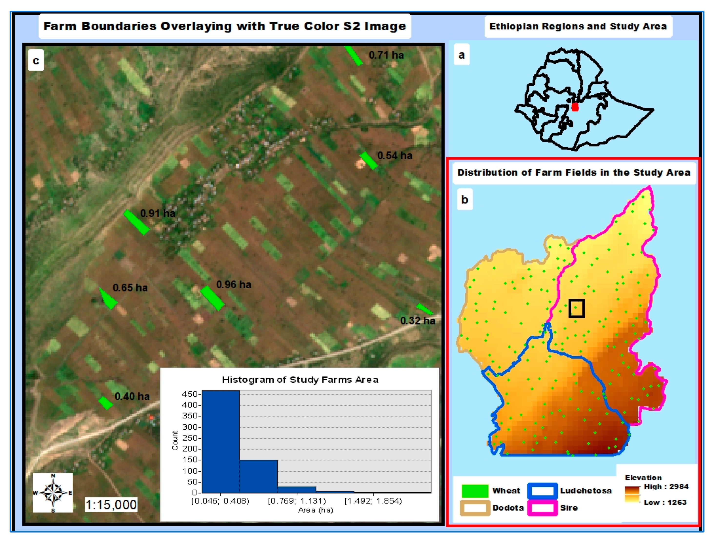
This study was located in one of the predominant wheat-growing regions of central Ethiopia (Figure 1a), which covers three districts (locally known as weredas): Arsi Sire, Dodota, and Ludehetosa (Figure 1b). The total area coverage is estimated to be 125,492 ha. Though elevation ranges between 1263 and 2984 m above sea level (masl), low- and mid-altitude landscapes dominate (Figure 1b). The farming system of the study area is characterized as rainfed and smallholder; this study selected 165 wheat farm fields through randomization (Figure 1b). The area of the study farms spans from 0.12 to 2.13 ha, with an average area of 0.53 ha, and most of them, as shown in the histogram in Figure 1c, have an area that is less than the average farm size.
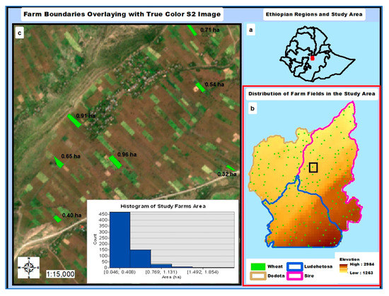
Figure 1.
Location of the study area (a), study districts (b) and farm distribution (points) (b) as well as some farm boundaries (polygons), (c) and histogram of study farm areas.
2.2. Dataset Description
In this study, two major groups of datasets were applied: field-collected agronomic data and satellite images. The major field-collected data included yield harvest, input utilization (fertilizers and herbicides), and crop calendar data. Wheat fields that were selected through randomization were demarcated using GPS (Global Positioning System), and the accuracy of each farm’s unit boundaries was checked and corrected by overlaying the polygons on Google Earth.
The study applied S2 and S1 images, which represent the optical and synthetic aperture radar (SAR) groups of satellite sensors, respectively. Sentinel-2 images are higher resolution (10 m spatial and 5-day temporal resolutions), while S1 SAR images equipped with a C-band have a spatial resolution of 10 m and temporal resolution of 12 days. Temporally, this study focused on the year 2020 during the major crop growing season, which spans from July to November. The multispectral analysis of the S2 data focused on the post-grain-filling period, which is a critical period for wheat yield prediction [21,22]. The specific dates that were analyzed were 5 October 2020, 10 October 2020, 15 October 2020, and 20 October 2020. On the other hand, the S1 data analysis included the whole wheat-growing period and considered 12-day intervals. Seven S1 images taken from 4 August to 27 October 2020 were used in this analysis. Based on wheat phenology, images from the dates 4 August 2020–21 September 2020 represent the tillering and grain-filling stage, while those from 3 October 2020–27 October 2020 represent the post-grain-filling stage [23].
2.3. Sentinel-2 Preprocessing and Vegetation Indices
The retrieved raw S2 images were preprocessed from level-1C to level-2A using the SNAP atmospheric correction algorithm. A resampling procedure was applied to obtain quality scene classification output, which was then used to prepare the cloud mask layer. The presence of many vegetation indices revealing various levels of accuracy and potential for crop yield prediction resulted in it being difficult to pick the best-performing ones. Thus, to achieve a full representation of the various categories, eight indices from four major categories (green VI, water index, chlorophyll index, and biomass index) were applied [24,25]. The selected indices as well as with their respective formulae are presented in Table 1.

Table 1.
Vegetation indices with their major categories derived from Sentinel-2 images.
All the vegetation indices were derived using the SNAP platform in the Thematic Land Processor. The green, water, and chlorophyll indices were computed under the toolsets of the radiometric vegetation index and water radiometric index processors, while the Dry Biomass Indices were computed using a biophysical processor.
2.4. Sentinel-1 Data Processing and SAR Indices
A total of 8 Level-1 Ground Range Detected (GRD) Sentinel-1A interferometric wide images with a 10m spatial and 12-day temporal resolution were downloaded from the Copernicus Open Access hub. Conventional SAR preprocessing operations, viz. applying the orbit file, thermal noise removal, radiometric calibration, multi-looking, speckle filtering, terrain correction, and radiometric normalization were applied. The output SAR data were then projected onto WGS 1984 Universal Mercator (UTM) coordinates for further processing.
Sentinel-1 data are available both in single- and dual-polarization modes. This study refers to previous studies [33,34] and selectively applied σ0 during VH polarization, as it revealed higher potential as a crop yield predictor. The C-band of the polarimetric SAR data has a limited capability to penetrate into the crop canopy, making less affected by the soil background. Thus, these data were considered to be a suitable candidate for the biomass estimation of crops [34]. In this study, two groups of indices: the single-date and combined-date indices were derived using σ0 during VH polarization. The single-date indices were computed for each of the eight dates, whereas the SAR normalized difference index (SNDVH), SAR simple difference index (SSDVH), and SAR simple ratio index (SSRVH) were the combined-date indices (Table 2).
Table 2.
The five types of SAR indices used in this study.
2.5. Setting of Predictor Variables
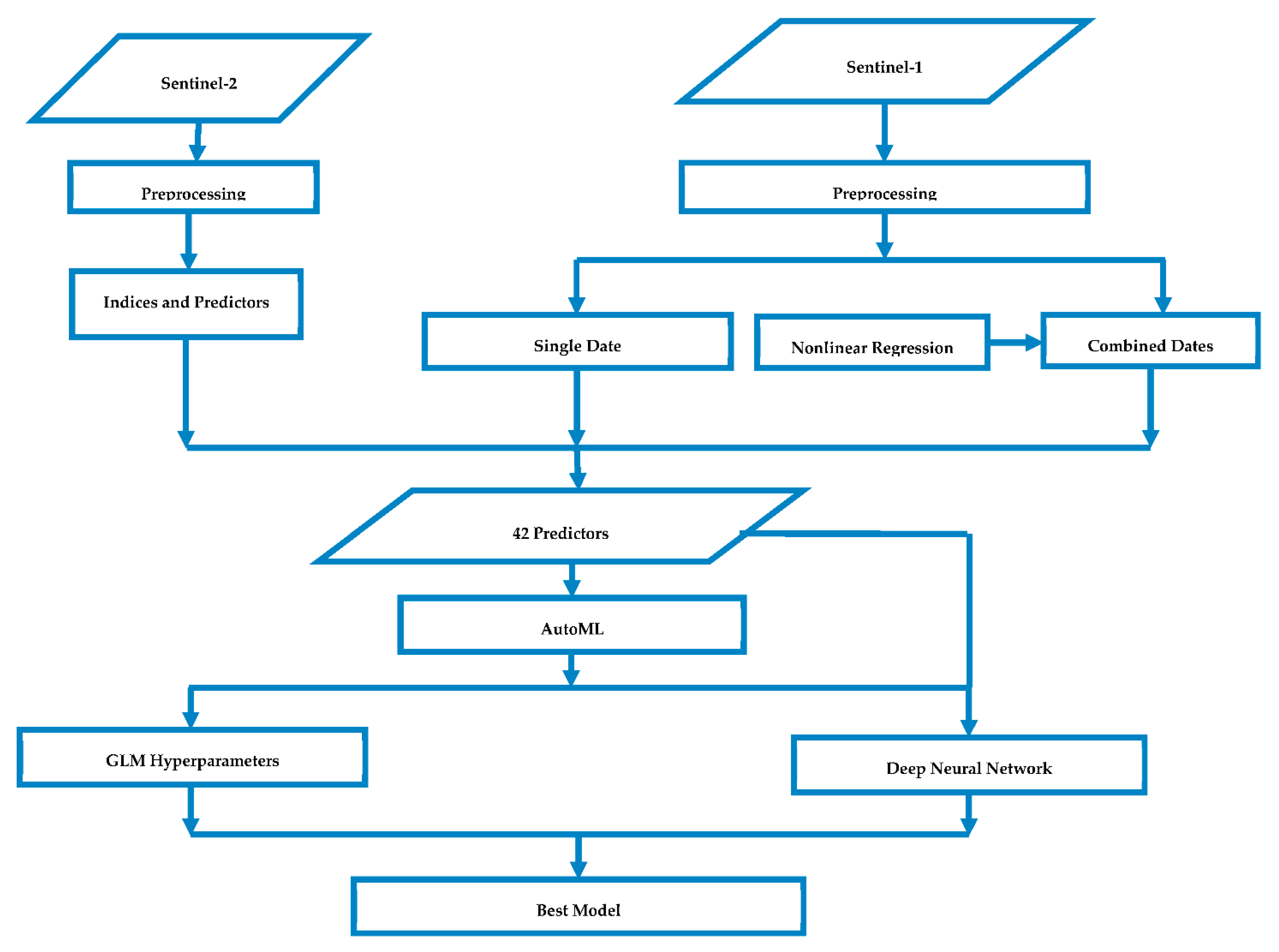
All of the vegetation indices derived from the S2 and S1 sensors, comprising a total of forty-two indices, were aggregated per farm boundary to set the final predictors. Thus, for each of the farms, a mean value of all of the pixel values per farm boundary was calculated. Then, the mean values for each farm unit were weighted per the farm area to standardize the per hectare area. Finally, these values were added as predictors to develop predictive regression models. The overall methodology followed by the study (from input to output) is presented in Figure 2.
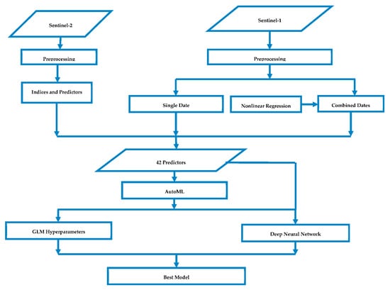
Figure 2.
Flow diagram showing the input dataset, derivation of predictors, and the three algorithms used.
2.6. Data Mining Methods
2.6.1. Nonlinear Regression (nlsLM)
In general, as presented in previous studies, there is an exponential relationship between the crop yield response and some SAR indices [33]. Thus, this study applied a non-linear model, which is abbreviated as nlsLM, to fit the relationship [35]. For the response variable (wheat yield (ton/ha)), as part of data preprocessing, outliers were identified and removed. Due to the small number of observations employed, a leave-one-out cross-validation (LOOCV) technique was applied. LOOCV is a special case of the k-fold cross-validation technique in which the number of folds is the same as the number of observations. It reduces bias and randomness and controls overfitting, and it offers a comprehensive evaluation, as it uses all of the samples for validation. The model’s goodness of fit was assessed using the root mean square error (RMSE) and leave-one-out cross-validation root mean square error (LOO RMSE) [36].
2.6.2. Machine Learning Models
Machine learning algorithms have been effective in modeling the complex relationship between predictor variables and crop yield. Among the available options, this study applied the H2O machine learning platform, as it is in the public domain and includes various machine learning algorithms [37]. For the effective and systematic exploitation of the platform, we applied three methods: AutoML (automated machine learning), GLM (generalized linear model), and deep learning. Automated machine learning methods are more recent algorithms that are becoming increasingly popular. Automating the end-to-end machine learning process enables quick and straightforward solutions and models. The AutoML process in H2O provides a model explainability interface that enhances our understanding of the learning process against the very black-box nature of machine learning methods. Another interesting feature of H2O’s AutoML process is that it is designed as a package that contains various sub-algorithms, including GLM (generalized linear models), GBM (gradient boosting machine), DRF (distributed random forest), XRT (extremely randomized trees), deep learning, and stacked ensembles. The steps of the learning process applied in this study are as follows: First, an AutoML was implemented using a dataset partitioned into 80:20 ratios for training and testing, respectively. Second, the top algorithm from AutoML was picked for further in-depth hyperparameter optimization in a stand-alone GLM model. This process was repeated 30 times, and the hyperparameters with the lowest RMSE values and that appeared more frequently on both the training and test datasets were selected as the best ones. The number of repetitions kept at 30 because, in general (even though it was possible for some parameters to be determined earlier), it was possible to determine the most frequently appearing best values across the hyperparameters at that point.
Then, the best hyperparameters were applied using 80:20 ratios for training and testing. Due to the stochastic nature of machine learning methods, with every run of an algorithm potentially giving a different output, mean values were reported with their confidence intervals. As the nature of the population distribution and standard deviation of the population are unknown, the t-interval was used. Therefore, the algorithm was run 30 times, which is the minimum number of samples required to apply the t-interval.
2.6.3. Deep Learning
This study implemented a deep learning algorithm using the total number of forty-two predictors as well as the 10 most influential predictors obtained from AutoML. The learning process of deep learning models may involve searching for the optimal values of many parameters. However, in this study, the learning process focused on the architecture of the neural network and on controlling overfitting problems. Moreover, as deep learning in H2O uses an adaptive learning rate, it does not require tuning. To exploit the potential of the algorithm, the study followed the following steps:
- Search for an optimal number of neurons for one, two, and three hidden layers using a separate setup for each using a grid with a random discrete search strategy using the training dataset.
- Search for the optimal values of the hyperparameters, such as type of activation function, hidden dropout ratios, input dropout ratios, l1 regularization, and l2 regularization, using the training dataset. The range of the values that were searched is presented in Appendix A.
- Select the best combination of tuned hyperparameters and apply them to the training, cross-validation, and the test datasets.
- Tweak parameters for controlling overfitting, such as hidden dropout ratios, input dropout ratios, l1, and l2, using the training, CV, and test datasets.
- Apply the final selected parameters thirty times (due to stochasticity) and compute the CI for the mean value.
3. Results
3.1. Non-Linear Data Modeling between Wheat Grain Yield and SAR Indices
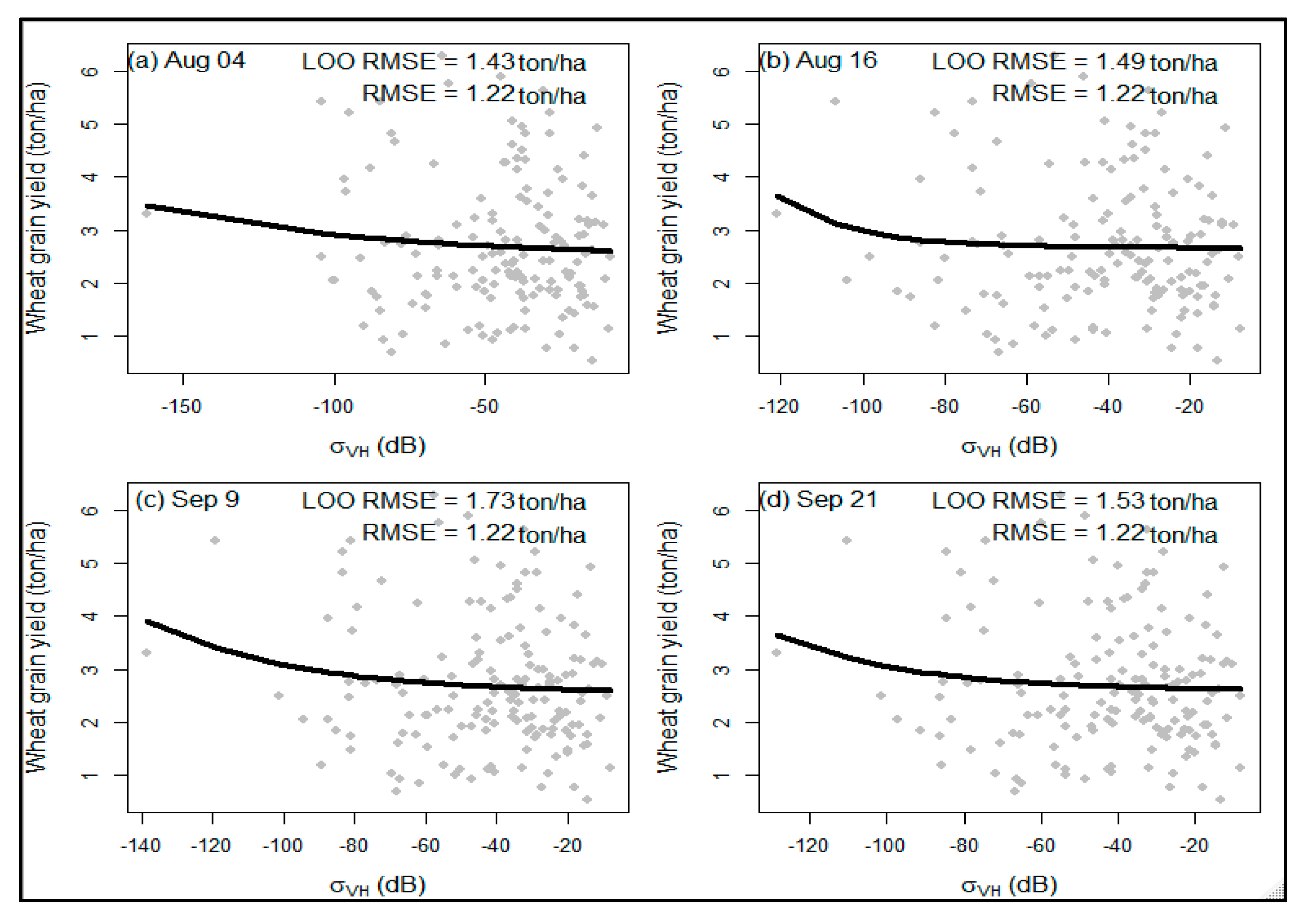
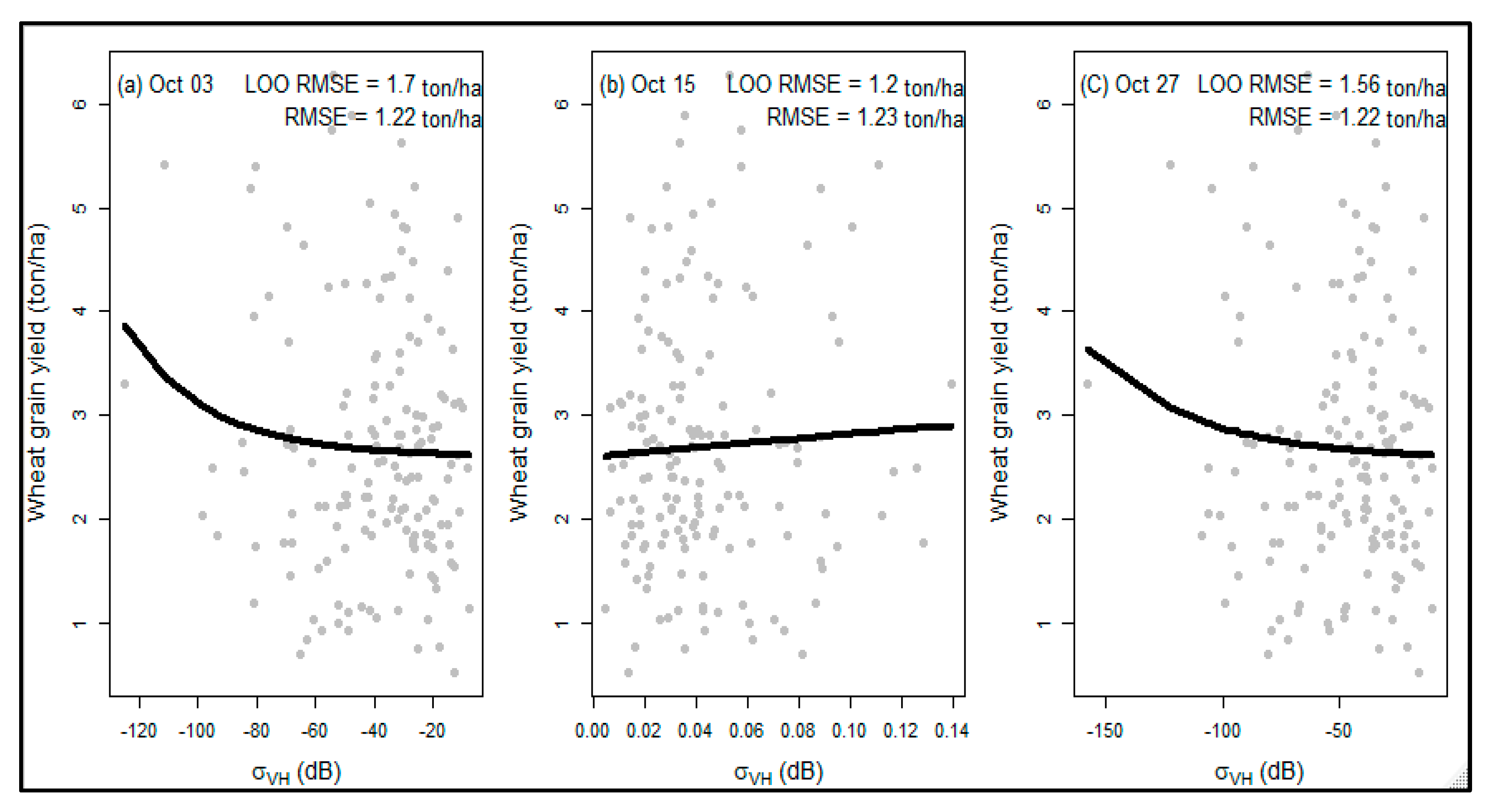
Based on the non-linear modeling, there is an exponential relationship between the single-date SAR indices and the wheat grain yield (ton/ha). Figure 3 shows the results of the non-linear model plots (represent by black fitting lines) for four dates within the tillering and grain-filling growth stage (Figure 3a–d represent non-linear models for the dates of 4 August, 16 August, 9 September, and 21 September, respectively). On the other hand, the three plots in Figure 4 present outputs for three dates: 3 October (Figure 4a), 15 October (Figure 4b), and 27 October (Figure 4c) for the post-grain-filling stage. The comparisons between the two stages: the tillering and grain-filling stage (Figure 3) and post-grain-filling stage (Figure 4), revealed a closer result. Across all of the dates and the two growing stages, the RMSE, with one exception (Figure 4b with 1.23 RMSE value), was 1.22 ton/ha, whereas the LOO RMSE ranged from 1.22 ton/ha to 1.73 ton/ha, showing closer results between the stages. In general, across the two stages, the plots between the single-date σ0VH,F and σ0VH,P indices and wheat grain yield (ton/ha) revealed an exponential function.
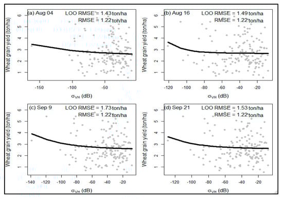
Figure 3.
Scatter plots of SAR indices of single growth stage (x−axis) vs. grain yield (y−axis) for tillering and grain-filling stage.
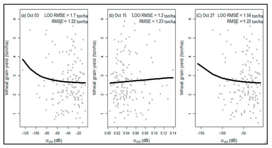
Figure 4.
Scatter plots of SAR indices of single growth stage (x−axis) and grain yield (y−axis) for post-grain-filling stage.
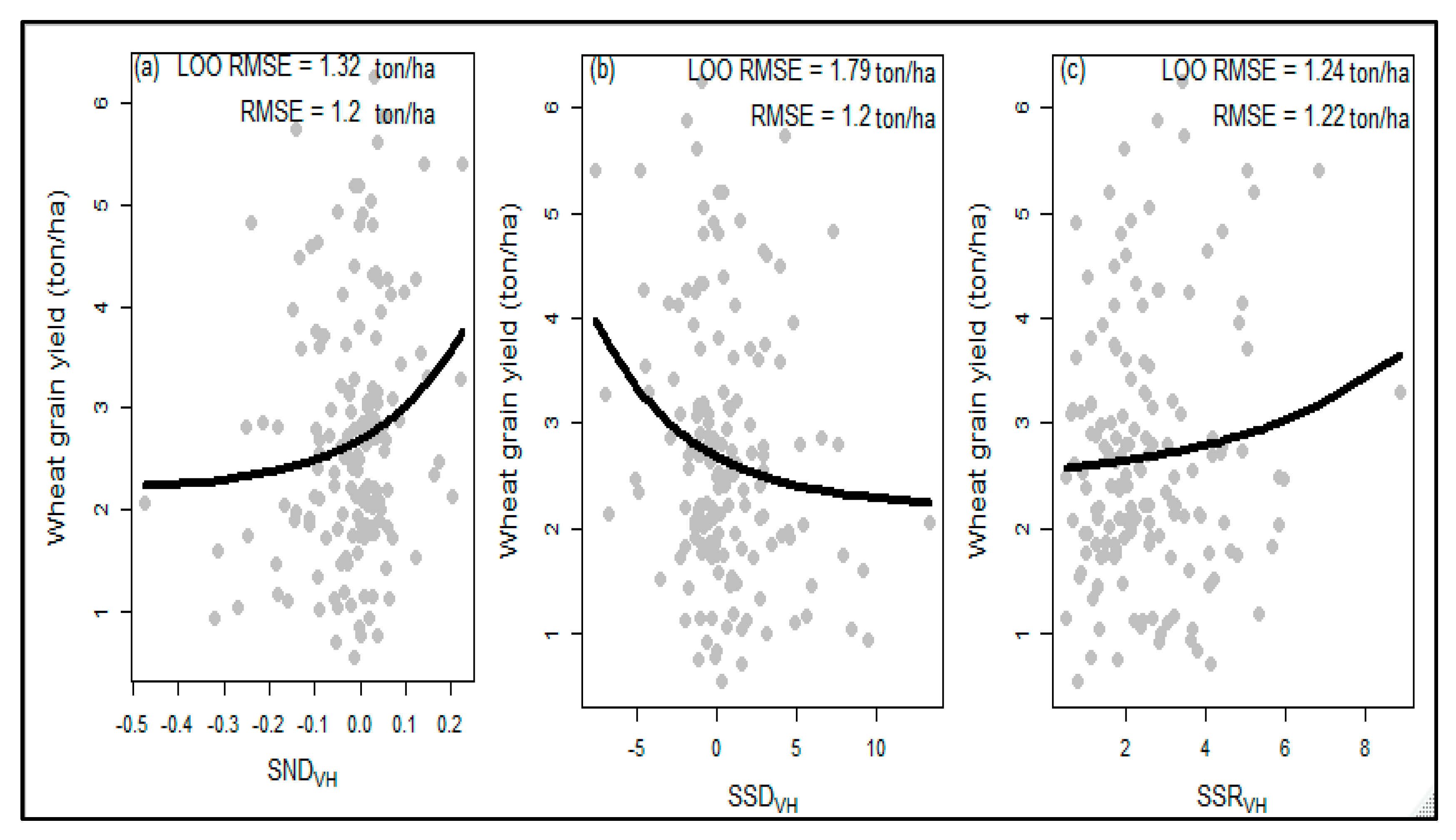
Similar to the single-date indices, the combined-date VH polarized indices resulted in an RMSE of 1.2 ton/ha (Figure 5). Nonetheless, the SND (Figure 5a) and SSR (Figure 5c) showed better performance and revealed closer values between LOO RMSE and RMSE, implying the absence of overfitting. For SND (Figure 5b), the LOO RMSE and RMSE achieved results of 1.32 ton/ha and 1.24 ton/ha, respectively. For SSR, 1.20 ton/ha and 1.22 ton/ha were obtained for the LOO RMSE and RMSE, respectively. Conversely, the SSD model had an RMSE of 1.2 ton/ha compared to a higher value of 1.79 ton/ha for the LOO RMSE. The higher value of the LOO RMSE could be due to the presence of more noise in the dataset, which, in turn, is associated with the wider data range in the SSD value (−5–10).
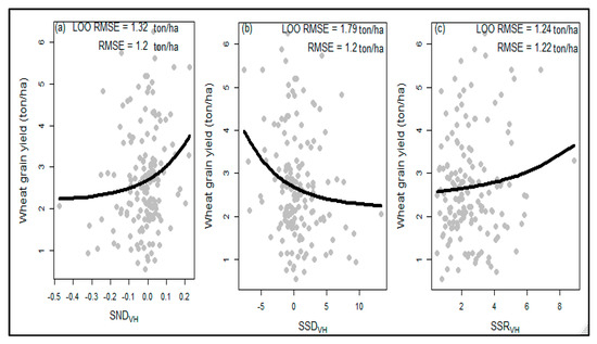
Figure 5.
Scatter plots showing the non-linear models for three indices using combined-date VH polarization (db). Sub plots (a–c) represent non-linear model results of the SND, SSD, and SSR indices, respectively.
3.2. Modeling Using AutoML
Automated machine learning, AutoML, offers a quick method for training and can achieve satisfactory results in a short amount of time. In this study, the process of training an AutoML started by using all forty-two variables as predictors. To obtain conclusive output, AutoML training was implemented repeatedly. Out of the ten runs of the AutoML method, the GLM model, which is one of the components of the AutoML method, was the top-performing one as it came first in seven cases (see Table 3 for an average value of the ten runs).
Table 3.
Table showing the performance of the top four component algorithms of the AutoML model.
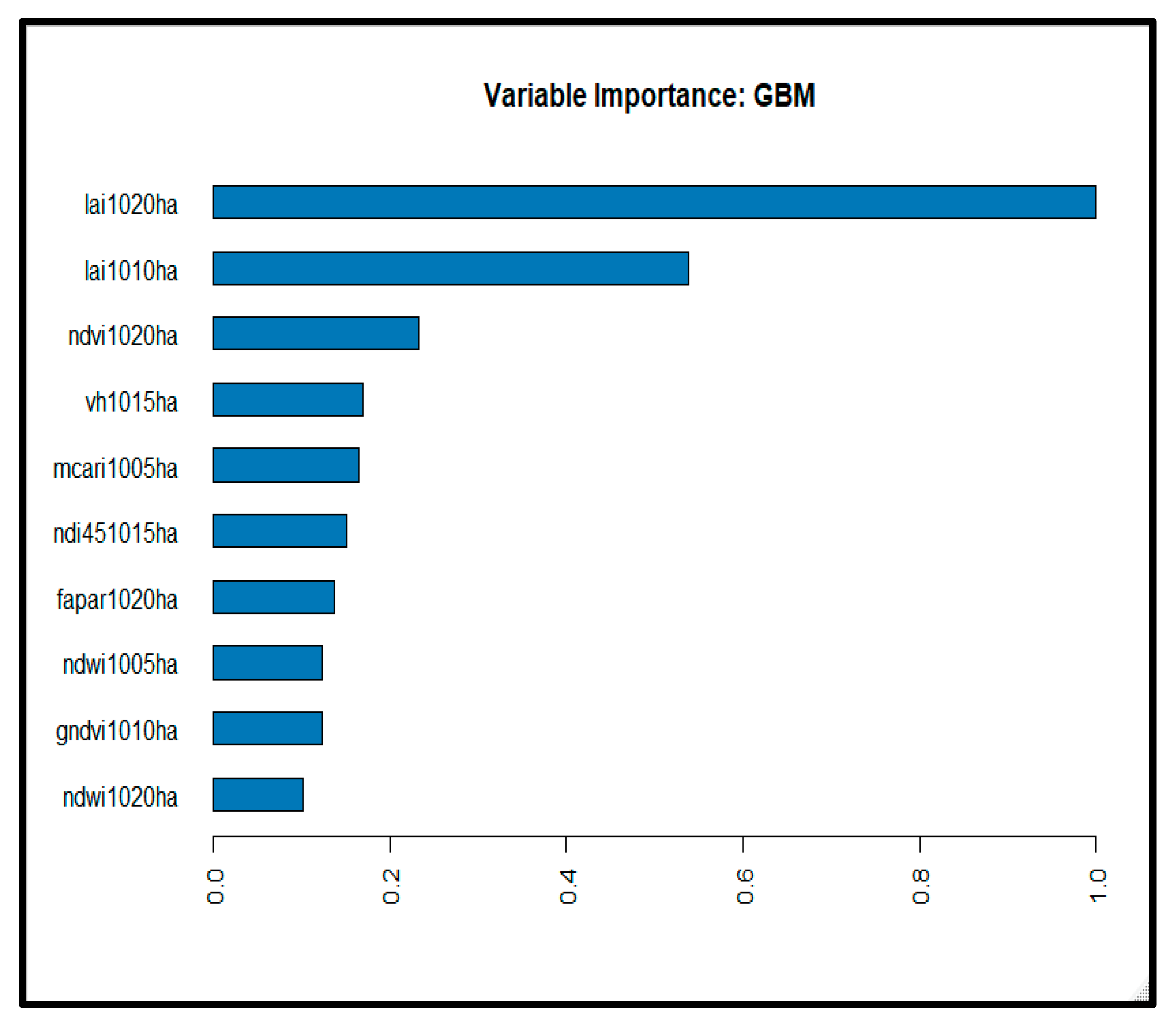
According to the average values, the GLM 1 model revealed average values of 0.93 ton/ha, 0.87 ton/ha, and 0.74 ton/ha for the RMSE, MSE, and MAE, respectively. The stacked Ensemble Best of Family algorithm was the second-best performing algorithm. Various GBM were also among the top algorithms, and, most importantly, they constitute the top models, appearing repeatedly at the top of the list. Given the small number of observations in this study on the one hand and the large number of predictors on the other hand, it is imperative to select the most important variables. Thus, according to the variable importance plots developed using the two best performing models, viz. GLM (see Appendix B) and GBM (see Appendix C), the ten most important variables were selected: LAI1020, LAI1010, NDVI1020, VH1015, MCARI1005, NDI451015, Fapar1020, NDWI1005, GNDVI1010, and NDWI1020. Of all of the predictors, LAI became the most influential predictor. Moreover, the predictors derived from S2 were found to be more important than those derived from the S1 sensors.
3.3. Modeling and Validation of GLM Model
The most important variables were selected using an AutoML algorithm. The GLM model was found to be the top model compared to the other components of the AutoML. In this section, to fully exploit the potential of the GLM model, hyperparameter tuning was implemented by employing the top ten most important variables. For the GLM model, alpha was the most important hyperparameter; a grid search process was implemented to obtain the best value of alpha and the corresponding lambda value. Thus, alpha = 0.0 and lambda = 0.02808 were found to be the best hyperparameters. These hyperparameters were applied using five-fold CV. Due to the stochastic nature of the machine learning algorithms, we determined the CI for the population mean (Table 4) of wheat yield. Accordingly, we achieved a 99% confidence level for the unknown RMSE (ton/ha) of the mean of the population on the training dataset, with a value of 0.84 to 0.88. Likewise, for the test dataset, the 99% CI was 0.84–0.98.
Table 4.
Table showing RMSE (ton/ha) CI values of 99% for training, CV, and test datasets.
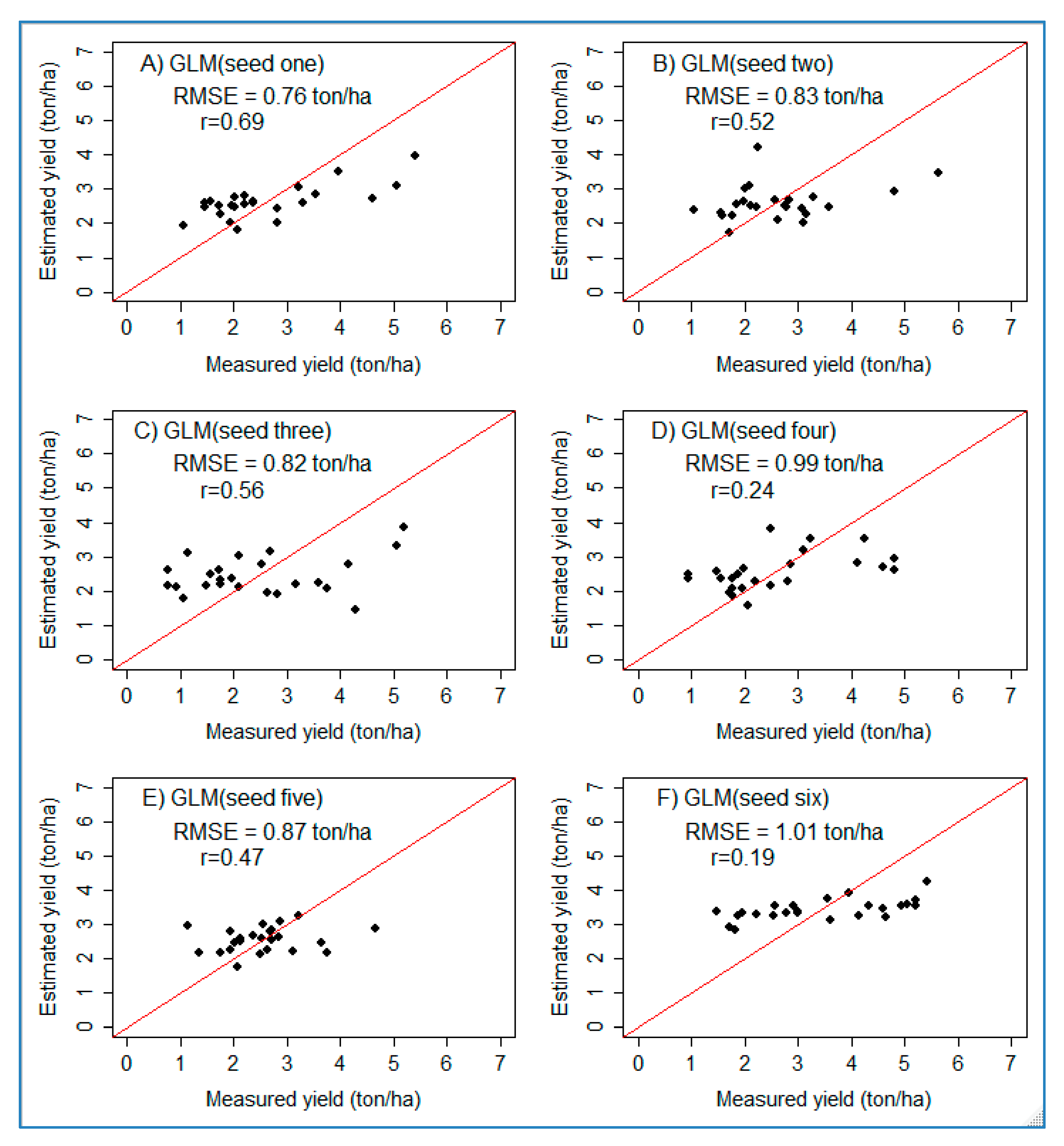
In addition to the average values that were reported, scatter plots were also helpful to examine the correlation between the estimated (predicted) and measured yields. For the test dataset, six scatter plots for six GLM models using different seeds were computed (see Figure 6). Accordingly, the correlation coefficient (r) between the estimated and measured yield ranges from 0.69 to 0.19. Since the study was implemented using a small dataset domain, careful handling of the outliers is critical, and outliers were removed.
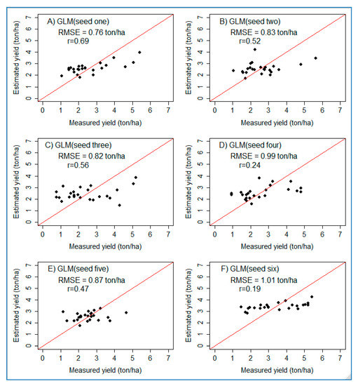
Figure 6.
Scatter plots showing the performance of GLM on the test dataset for six randomly selected seeds. The red lines represent a 1:1 line between estimated and measured yields. (A–F) refer to six plots prepared using six randomly generated numbers (seeds).
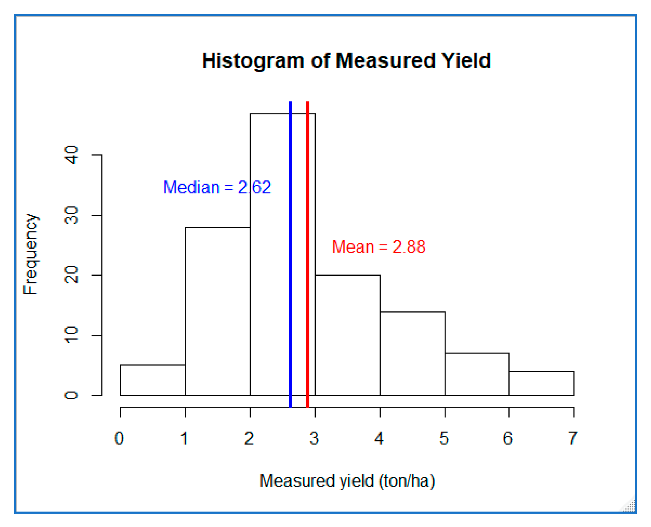
However, by summarizing the information from the six scatter plots, it can be observed that the performance of the models is weak at higher yield values (beyond 4 ton/ha). This could partly be associated with the non-normal sample distribution property of the response variable (measured yield). The response variable has an average value of 2.88 ton/ha and a median of 2.62 ton/ha, which are almost the same. However, the dataset has a range of 0–7 ton/ha, and this resulted in the histogram being skewed to the left (see Figure 7). Even after outliers were removed, the models showed limitations at higher values.
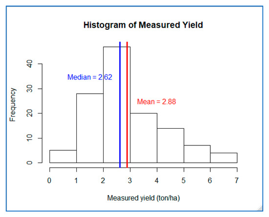
Figure 7.
Histogram of measured yield with mean and median values.
3.4. Modeling and Validation of Deep Learning
When applying deep learning models, the number of neurons is the most important parameter. In this study, tuning for the optimal values for the number of neurons was implemented separately for one, two, and three hidden layers. In general, among the three groups, models with two hidden layers were inferior. Since the purpose of this study was to find the best model, the results below focus on the other two groups; however, the summary for all three groups will be presented later on (Table 5). Accordingly, for one hidden layer, as shown in Figure 8, two major characteristics were observed. Initially, as the number of neurons increased the error decreased; however, it started to increase as the number of neurons increased further. In particular, the error values increased steadily as the number of neurons passed a value of 1000. Thus, the number of neurons in the region where the global minimum was expected ranged from 0–1000.
Table 5.
Table showing the number of neurons of the lowest three error values for three hidden layers.
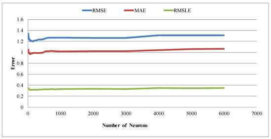
Figure 8.
Table showing the number of neurons against error metrics (RMSE, MAE, and RMSLE) for one hidden layer in the validation group. The three metrics are average values.
As a result, out of the total range (0–7000), the learning process targeted the limited range (0–1000) to identify the global minima value. Thus, detailed learning was implemented, and results are displayed using Figure 9.
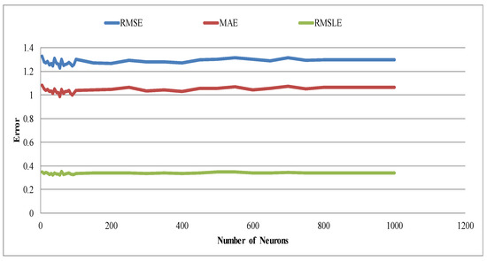
Figure 9.
Table showing the number of neurons for the range of 0–1000 against error metrics (RMSE, MAE, and RMSLE) for one hidden layer in the validation group. The three metrics are average values.
Likewise, Figure 10 presents the performance for three hidden layers. Based on the three metrics used, lower error metrics were found when the number of neurons was less than 100.
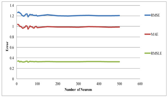
Figure 10.
Table showing number of neurons against error metrics (RMSE, MAE, and RMSLE) for three numbers of hidden layers in the validation group. The three metrics are average values.
In the previous section (Figure 8, Figure 9 and Figure 10), the overall trend of the number of neurons against the error metrics was presented. To identify the optimal number of neurons yielding the lowest error value, the lowest three error values for each of the three hidden layers were computed (Table 5). The comparison across the three groups of hidden layers showed that 55 number of neurons of the three hidden layer group revealed the lowest MAE and RMSE values of 0.95 ton/ha and 1.18 ton/ha, respectively.
Nonetheless, for one hidden layer 80 and 75 neurons revealed an RMSLE value of 0.31 ton/ha, which was the lowest one in the group.
Therefore, for subsequent parameter tuning, 80 neurons were selected for one hidden layer, and 55 neurons were selected for three hidden layers. Among the various hyperparameters available for deep learning, in this study, we selected the most important ones: the type of activation function, the hidden dropout ratio, output dropout ratio, l1 regularization, and l2 regularization. These parameters were searched using a grid search strategy, and the optimal hyperparameters were obtained and are presented in Table 6. In both groups, tanh drop out activation function and input dropout ratio values of 0.5 are the best values.
Table 6.
Optimal hyperparameters selected based on performance on training, CV, and test datasets.
Finally, for two hidden layers, the best hyperparameters were applied, and the CI was computed. Thus, Table 7 and Table 8 revealed that the mean RMSE of wheat yield at a 99% CI for one and three hidden layers, respectively. For the networks with one hidden layer, the RMSE on the training dataset was 1.24 ton/ha, while a value of 1.42 ton/ha was obtained on the test dataset. This result was obtained using the total number of predictors (42) used in the study.
Table 7.
Showing RMSE (ton/ha) values at a 99% CI for the training, CV, and test datasets for one hidden layer.
Table 8.
Table showing RMSE (ton/ha) values at 99% CI for training, CV, and test datasets for three hidden layers.
Compared to the outputs obtained using one hidden layer, three hidden layers revealed better outputs. As shown in Table 8, mean RMSE values of 1.20 ton/ha and 1.34 ton/ha were obtained using the training and test datasets, respectively. These values were obtained using 10 predictors identified based on their variable importance using the AutoML algorithm presented under Section 3.2. Although the ten parameters were applied for one hidden layer, the performance did not improve.
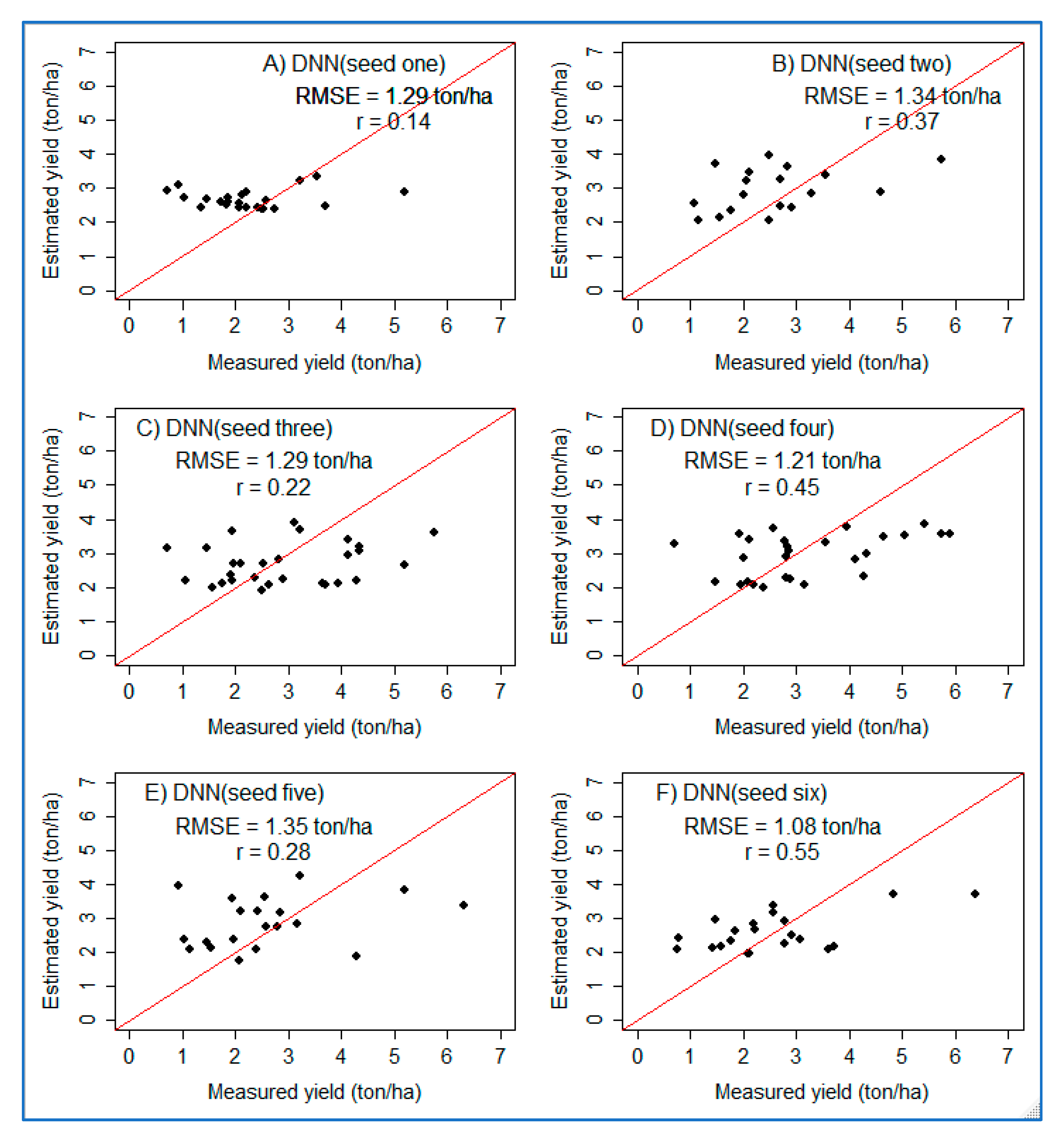
In addition to metric-based validation, model performance was assessed using scatter plot analysis. As shown in Figure 11, six scatter plots for six DNN models using three hidden layers using the test dataset were prepared. The scatter plots present the correlation between the estimated yield and measured yield. In general, there is a positive correlation, and a strong association is displayed in the range of less than 4 ton/ha. Similar to the GLM model performance discussed in Section 3.4, the DNN model showed limitations at higher values.
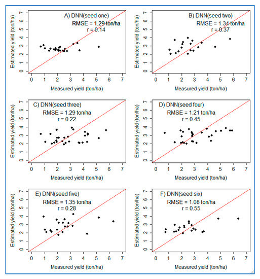
Figure 11.
Scatter plots showing the performance of DNN with three hidden layers on the test dataset for six randomly selected seeds. (A–F) refer to six plots prepared using six randomly generated numbers (seeds).
4. Discussion
This study aimed to develop a method for remote sensing-based wheat yield prediction in smallholding and heterogeneous farming systems. The study obtained predictors from vegetation indices derived from high-resolution optical and SAR sensors. Eight vegetation indices were computed from S2 optical sensors, and five SAR indices were calculated from the S1 sensor data. Considering the complex relationship between the predictors and response variables, data mining methods, which can be grouped under three broad categories: statistical, machine learning, and deep learning, were applied. Unlike common approaches to machine learning and deep learning implementation, due to the scarcity of the response variable (field-collected wheat grain yield), in this study, data mining methods were implemented under a small dataset domain.
In harnessing the phenological information of the wheat, VH backscatter SAR indices were computed for single and combined dates. Single-date indices were calculated for two stages: the tillering and grain-filling stage and the post-grain-filling stage. For both stages, as determined in previous studies [33], an exponential relationship existed between the single-date SAR index and wheat grain yield. The non-linear modeling of the two stages revealed closer outputs. For the two stages, the LOO RMSE ranged between 1.22 ton/ha and 1.73 ton/ha, while the RMSE was 1.22 ton/ha. The similarity of the outputs from the two stages suggests that the SAR indices could be used by either of them, offering comparable results.
The smaller gap between the RMSE and LOO RMSE values, the combined-date indices, such as SND and SSR showed relatively improved performance over the rest of the SAR indices. SND and SSR achieved values of1.32 ton/ha and 1.20 ton/ha as well as values of 1.24 ton/ha and 1.22 ton/ha for LOORMSE and RMSE, respectively. This shows that the combined-date indices offer increased capacity over single-date indices. It is intuitive to expect indices to integrate wider phenological information to outperform narrow ones.
Overall, in this study, the performance of the SAR indices as wheat yield predictors compared to other predictors is weak. Since the SAR parameters are sensitive to many biophysical variables, including the plant structure, leaf size, stem density, biomass, and plant water content, they have immense potential to determine important crop parameters [38]. Nonetheless, the application of the SAR signal in agriculture is complicated, as the signal is sensitive to soil moisture and surface roughness, and SAR backscatter is also influenced by the inherent properties of the SAR signal, such as its frequency, incidence angle, and polarization [39]. On the other hand, some previous studies revealed strong prediction capability. For instance, using the SSDVH predictor, rice yield was estimated with RMSE value of 0.74 ton/ha and with a relative error of 7.93% [33].
For wheat, it was asserted that the relationship between the polarimetric SAR parameters and wheat height is complex. Weak correlations are reported at the early and late growth stages. At the stem elongation stage, relationships are negative, and correlations are weak between most of the polarimetric SAR parameters and wheat height. A relatively good but negative association with wheat height was revealed using HV and Yamaguchi helix scattering with R2 = 0.57 and R2 = 0.39, respectively, during the middle growing stage [40].
Among the constituent algorithms of the AutoML package, the GLM and GBM yield improved performance. Using the ten influential parameters, the GLM model revealed an RMSE of 0.84–0.98 ton/ha for the mean population at a 99% CI on the test dataset, while the performance on the training dataset was 0.84–0.88 ton/ha. The narrower gap between the two performances implies that the model has a good generalization error. This model used an alpha value of 0 and a lambda value of 0.02808. An alpha value of 0 represents ridge regression that is theoretically expected to offer better results when the prediction power is spread out over the various features. This is well-observed in this study, where a number of predictors were found to be important (see Appendix B).
Among the 42 predictor variables derived from both optical and SAR indices covering the tillering and grain-filling stage and post-grain-filling stage, in the post-grain-filling stage (i.e., LAI1020), the leaf area index is the most influential parameter. In maize fields, the leaf area index obtained from field instrument measurements outperformed fifteen vegetation indices, showing a higher association with biomass, with R2 = 0.89, RMSE = 2.27 ton/ha, and RRMSE = 30.55%. In particular, in good agreement with this study, the leaf area index obtained during the grain-filling stage (relative root mean squared error (RRMSE) = 29.83%) shows improved performance over early stages (RRMSE = 38.87%) [16]. Likewise, the LAI from the Sen2-Agri estimates derived using inverse radiative transfer modeling revealed better capability than various vegetation indices, with R2 values of 0.68, 0.62, 0.80, and 0.48 for cotton, maize, millet and sorghum, respectively [24]. This implies that the S2-derived leaf area index is good enough for monitoring yield variability and can be used to replace the field-measured leaf area index. On the other hand, the rest of the predictors representing the green, water, and chlorophyll index groups showed closer potential and were inferior to the biomass indices (in this case, the leaf area index).
The present study implemented a deep learning model emphasizing the architecture of the neural network. Due to their inherent complexity, deep learning models are likely to overfit during training. This is especially more likely when using a small dataset. Deep learning models apply several regularization techniques to control overfitting. This study applied the three widely applied regularization techniques: L1, L2, and dropout. In general, regularization techniques, when applied in deep learning models, offer a robust model via reducing the complexity of the network. L1 regularization forces the weight parameter to become zero, whereas L2 forces the parameters towards zero. Dropout methods make the training process noisy. In neural networks, dropouts are implemented per layer, i.e., on hidden layers and on the visible or input layers. In this study, three number ranges of neurons: 0–6000, 0–1000, and 0–500, were searched for one, two, and three hidden layers. A model with three hidden layers with 55 neurons each and with the tanh dropout activation function showed improved performance. At a 99% confidence interval, the mean RMSE was 1.31–1.36 ton/ha on the test dataset. Moreover, this model had hidden dropout ratio, input dropout ratio, and l2 regularization values of 0.1, 0.5, and 0.00001, respectively.
On the other hand, the model with one hidden layer revealed a 99% CI of 1.41–1.43 ton/ha for the mean RMSE. The optimal hyperparameter values of the model are 80 neurons, the tanh dropout activation function, a hidden dropout ratio of 0.5, an l1 regularization value of 0.1, an input dropout ratio of 0.5, and an l2 regulation value of 0.1. The deep learning model using three hidden layers had a 99% CI of 1.31–1.36 ton/ha for the mean RMSE and outperformed the model with one hidden layer, indicating that this could be associated with the former model that used the ten most influential parameters and the later model using the full set of predictors. Nonetheless, the combination of the ten influential parameters with a model with one hidden layer did not show any improvement over using the full number of predictors.
Deep learning methods are applied because they are expected to deliver better results compared to machine learning algorithms. Comparing the machine learning and deep learning approaches for crop yield prediction is not a straightforward process. This is because the design and implementation of various studies are characterized by a diverse set of factors, viz. different algorithms, data sources, platforms, crop types, features (data groups), categories, and evaluation performance metrics. Moreover, there is also diversity in the motivation of deep learning, such as processing multiple array formats in nonlinear modules, integrating multiple parameters accurately, automating and/or simplifying tasks, capturing time dependencies, and the capability of generalizing and revealing superior models [19]. Nonetheless, there are some relevant studies. Convolutional neural network (CNN), deep neural network (DNN), and long short-term memory (LSTM) are the best-performing deep learning algorithms used in crop yield prediction. Wheat is second to maize in terms of the most studied crop in deep learning. Supervised deep learning is the most widely applied deep learning method for crop yield prediction [19].
With the ultimate objective of developing a better model, this study applied three major methods, namely the non-linear model, automated machine learning, and a deep learning model. Among the constituent algorithms of the AutoML package, the GLM model was the top one. Thus, the study proceeded with the GLM model via hyperparameter tuning, which resulted in a significant improvement, causing it to outperform the rest of the models. Accordingly, a GLM model employing the ten most influential parameters revealed the best prediction results. Thus, the developed method employs both the capability of the AutomL package as well as the capability of GLM to search for hyperparameters. In terms of performance, revealing higher wheat prediction capability, this combined approach seems synergetic and fast compared to deep learning and non-linear models. Moreover, as the study was implemented under a small dataset and because the AutoML offered the ten most influential parameters, this contributed to the obtained performance improvement. From a practical perspective, this has invaluable significance. The efficient and effective training of machine learning models is often a very daunting task. Nonetheless, in this study, better results were obtained using an automated machine learning method that can be easily implemented by experts with limited skills in data mining methods. This implies the scalability of the approach to environments with limited access to well-skilled experts and robust off-the-shelf data mining platforms.
The comparison of the performance of the three data mining methods should be considered under the context and purpose of the study. First, the results from the nlsLM model were inferior to those of other models, mainly because it only used one type of predictor (derived from SAR). Initially, this method was chosen by referring to previous studies in which robust prediction capability was reported, hence causing it to be selected as a stand-alone method [33]. However, as the variable importance plot (see Appendix B and Appendix C) showed the importance of several predictors, the use of a single predictor might not offer satisfactory results. Second, for the combined method, an AutoML with tuned GLM, was the superior model. This was largely because it was determined the AutoML method offers a better fitting model after comparing the range of sub-algorithms that constituent the model. For instance, in this study, the AutoML revealed that the GLM model was better fitting compared to models such as the deep learning and stacked ensemble models, among others. Third, the performance of deep learning models should also be interpreted cautiously. This study applied a comprehensive (considering networks with one to three layers) and a rigorous (several hyperparameters) implementation approach. However, due to the wider complexity and resources of the deep learning models, different untested configurations might be possible and could unleash different capability.
The implementation of the current study under a small dataset domain resulted in both pros and cons. The advantages include, for instance, the LOOCV technique in nlsLM, which is theoretically expected to offer less biased model performance output, being easily implemented because the computational demand was inexpensive. In H2O platform’s reproducible results could be obtained using a deep learning algorithm if the system was deployed using a core and the same seed. In this regard, the use of a small dataset enabled availing reproducible results. Additionally, when the deployment of the algorithm did not offer reproducible results, for instance, the GLM model in H2O did not support reproducibility, the use of a small number of observations eased algorithms used to compute a CI from running repeatedly.
On the downside, machine learning and deep learning methods are commonly developed using big observation datasets, and the adoption of such methods under a small data set is associated with major constraints, such as controlling the bias-variance tradeoff, overfitting, and the careful handling of outliers. As a solution, in this study, several techniques were applied during data preprocessing, model development, and validation to address the constraints of the small dataset. Outlier removal and LOOCV were used during nlsLM modeling. Average values of error metrics were computed while the GLM and deep learning models were developed. Moreover, relevant predictors obtained from the AutoML model were used to develop the GLM algorithm. Furthermore, the mean and confidence interval values were computed to develop and validate the tuned GLM and deep learning algorithms.
5. Conclusions
This study was set to evaluate the potential of selected vegetation indices derived from Sentinel-2 and Sentinel-1 data as a wheat yield predictor. Moreover, it applied fast, reproducible, and open-source statistical, machine learning, and deep learning algorithms for wheat yield prediction under a small dataset domain.
The study successfully derived wheat yield predictors using optical (S2) and SAR (S1) sensors. The development of the indices considers the representation of important phenological information and various groups of indices. The study exploited the potential of three groups of data mining methods and presented fast and reproducible wheat yield prediction approaches.
A combined method, the AutoML with GLM hyperparameter tuning, showed higher performance over the rest of the methods. The AutoML, with minimum effort and within a short amount of time, was good enough to deliver the ten most influential parameters and was the top-performing algorithm among its constituents. The method revealed a mean RMSE of 0.84–0.97 ton/ha at a 99% CI using the ten parameters. The leaf area index obtained from the post-grain-filling stage was found to be the most influential parameter compared to all the rest of the optical and SAR-derived parameters.
Though the study applied a wide range of values for one, two, and three hidden layers, the lowest error metrics were found using a small number of neurons. A deep neural network with three hidden layers using the ten influential parameters outperformed networks with one and two hidden layers. It revealed a mean RMSE of 1.31–1.36 ton/ha on the test dataset at a 99% CI. This model used 55 neurons with hidden dropout ratio, input dropout ratio, and l2 regularization values of 0.1, 0.5, and 0.00001, respectively.
The optimal models obtained from the three data mining approaches take advantage of the phenological information, and the information from the post-grain-filling stage in particular.
Although various machine learning and deep neural networks have been developed and are widely available, the effective and efficient training of them is challenging. In this regard, the AutoML with GLM hyperparameters method is especially useful, as it is fast and reproducible and can potentially be applied in similar crop production systems. Moreover, it could be adapted to predict grain yields for other cereals crops using high resolution satellite sensors. Furthermore, as H2O is available under the public domain, it could be widely used in resource-poor setups. Future studies might compare the current approach and platform with widely used platforms for crop yield prediction, such as Keras and Tensorflow [19].
On the other hand, improved performance in terms of reliability and robustness could be sought by incorporating additional potential predictors that represent, for instance, soil and climatic variability, among others.
Author Contributions
Conceptualization, A.A.T., D.E.O.; methodology, A.A.T.; software, A.A.T.; validation, A.A.T., T.S.S. and B.G.A.; formal analysis, A.A.T.; investigation, A.A.T. and T.S.S.; resources, A.A.T., B.G.A. and D.E.O.; data curation, A.A.T.; writing—original draft preparation, A.A.T.; writing—review and editing, A.A.T., T.S.S. and B.G.A.; visualization, A.A.T.; supervision, D.E.O. and B.G.A.; project administration, A.A.T. and B.G.A.; funding acquisition, A.A.T., B.G.A. and T.S.S. All authors have read and agreed to the published version of the manuscript.
Funding
This study received financial support from Data Science Africa (DSA) grant award 2020 project.
Institutional Review Board Statement
Not applicable.
Informed Consent Statement
Not applicable.
Data Availability Statement
Sentinel-2 and Sentinel-1 data are available from https://earthexplorer.usgs.gov (accessed on 5 July 2021) and from the Copernicus Open access hub from https://scihub.copernicus.eu/dhus/#/home (accessed on 21 July 2021).
Acknowledgments
We are primarily indebted to Data Science Africa (DSA) for offering financial support for this research. We present our special appreciation to Ciira wa Maina, Dina Machuve, Mmubangizi, and Wacuka from Data Science Africa, who facilitated, followed up with, and monitored the administration of the fund and the project during the research period. We acknowledge to Ethiopian Space Science and Technology Institute for facilitating the management of the fund. We extend our appreciation to experts from Arsi-Sire, Dodota, and Ludehetosa, who supported the field data collection.
Conflicts of Interest
The authors declare no conflict of interest. The funders had no role in the design of the study; in the collection, analyses, or interpretation of data; in the writing of the manuscript; or in the decision to publish the results.
Appendix A
Table A1.
Table showing hyperparameters tuned with their range of respective values applied in the study for deep learning models.
Table A1.
Table showing hyperparameters tuned with their range of respective values applied in the study for deep learning models.
| No | Hidden Layer | Neurons | Activation Types | Hidden Drop out Ratios | Input Drop out Ratios | L1 | L2 |
|---|---|---|---|---|---|---|---|
| 1 | One | From 0–100 at an interval of 5, 100–800 at an interval of 50, 1000–6000 at an interval of 1000 | Tanh, tanh with dropout, rectifier, rectifier with dropout, maxout, maxout with dropout | 0, 0.1, 0.2, 0.5 | 0, 0.0001, 0.001, 0.05, 0.1, 0.2,0.5 | 0.00001, 0.0001, 0.01, 0.05, 0.1 | 0.00001, 0.0001, 0.01, 0.05, 0.1 |
| 2 | Two | From 0–100 at an interval of 5, from 100–800 at an interval of 50, and 1000 | Tanh, tanh with dropout, rectifier, rectifier with dropout, maxout, maxout with dropout | 0, 0.1, 0.2, 0.5 | 0,0.0001, 0.001, 0.05, 0.1, 0.2,0.5 | 0.00001, 0.0001, 0.01, 0.05, 0.1 | 0.00001, 0.0001, 0.01, 0.05, 0.1 |
| 3 | Three | From 0–100 at an interval of 5, from 150–500 at an interval of 50 | Tanh, tanh with dropout, rectifier, rectifier with dropout, maxout, maxout with dropout | 0, 0.1, 0.2, 0.5 | 0,0.0001, 0.001, 0.05, 0.1, 0.2,0.5 | 0.00001, 0.0001, 0.01, 0.05, 0.1 | 0.00001, 0.0001, 0.01, 0.05, 0.1 |
Appendix B
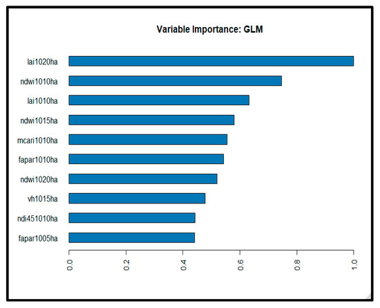
Figure A1.
A plot showing the top ten most influential variables using the GLM model.
Figure A1.
A plot showing the top ten most influential variables using the GLM model.

Appendix C

Figure A2.
A plot showing the top ten most influential variables using the GBM model.
Figure A2.
A plot showing the top ten most influential variables using the GBM model.
References
- Rapsomanikis, G. The Economic Lives of Smallholder Farmers: An Analysis Based on Household Data from Nine Countries; Food and Agriculture Organization of the United Nations: Italy, Rome, 2015. [Google Scholar]
- Knoema. Ethiopia—Wheat Imports. Available online: https://knoema.com/atlas/Ethiopia/topics/Agriculture/Trade-Import-Value/Wheat-imports (accessed on 22 July 2022).
- Atinafu, A.; Lejebo, M.; Alemu, A. Adoption of improved wheat production technology in Gorche district, Ethiopia. Agric. Food Secur. 2022, 11, 3. [Google Scholar] [CrossRef]
- Hammer, G. Applying seasonal climate forecasts in agricultural and natural ecosystems—A synthesis. In Applications of Seasonal Climate Forecasting in Agricultural and Natural Ecosystems; Springer: Berlin/Heidelberg, Germany, 2000; pp. 453–462. [Google Scholar]
- Hughes, N.; Lawson, K.; Valle, H. Farm performance and climate: Climate-adjusted productivity for broadacre cropping farms. ABARES Res. Rep. 2017, 17, 4–6. [Google Scholar]
- Verrelst, J.; Camps-Valls, G.; Muñoz-Marí, J.; Rivera, J.P.; Veroustraete, F.; Clevers, J.G.P.W.; Moreno, J. Optical remote sensing and the retrieval of terrestrial vegetation bio-geophysical properties–A review. ISPRS J. Photogramm. Remote Sens. 2015, 108, 273–290. [Google Scholar] [CrossRef]
- Dercon, S.; Gollin, D. Agriculture in African development: Theories and strategies. Annu. Rev. Resour. Econ. 2014, 6, 471–492. [Google Scholar] [CrossRef]
- Jin, Z.; Azzari, G.; Burke, M.; Aston, S.; Lobell, D.B. Mapping smallholder yield heterogeneity at multiple scales in Eastern Africa. Remote Sens. 2017, 9, 931. [Google Scholar] [CrossRef]
- Busetto, L.; Casteleyn, S.; Granell, C.; Pepe, M.; Barbieri, M.; Campos-Taberner, M.; Casa, R.; Collivignarelli, F.; Confalonieri, R.; Crema, A.; et al. Downstream services for rice crop monitoring in Europe: From regional to local scale. IEEE J. Sel. Top. Appl. Earth Obs. Remote Sens. 2017, 10, 5423–5441. [Google Scholar] [CrossRef]
- Aboelghar, M.; Arafat, S.; Yousef, M.A.; El-Shirbeny, M.; Naeem, S.; Massoud, A.; Saleh, N. Using SPOT data and leaf area index for rice yield estimation in Egyptian Nile delta. Egypt. J. Remote Sens. Space Sci. 2011, 14, 81–89. [Google Scholar] [CrossRef]
- Ndikumana, E.; Minh, D.H.T.; Nguyen, H.T.D.; Baghdadi, N.; Courault, D.; Hossard, L.; Moussawi, I.E. Estimation of rice height and biomass using multitemporal SAR Sentinel-1 for Camargue, Southern France. Remote Sens. 2018, 10, 1394. [Google Scholar] [CrossRef]
- Veloso, A.; Mermoz, S.; Bouvet, A.; Le Toan, T.; Planells, M.; Dejoux, J.-F.; Ceschia, E. Understanding the temporal behavior of crops using Sentinel-1 and Sentinel-2-like data for agricultural applications. Remote Sens. Environ. 2017, 199, 415–426. [Google Scholar] [CrossRef]
- Steele-Dunne, S.C.; McNairn, H.; Monsivais-Huertero, A.; Judge, J.; Liu, P.-W.; Papathanassiou, K. Radar remote sensing of agricultural canopies: A review. IEEE J. Sel. Top. Appl. Earth Obs. Remote Sens. 2017, 10, 2249–2273. [Google Scholar] [CrossRef]
- Harfenmeister, K.; Spengler, D.; Weltzien, C. Analyzing temporal and spatial characteristics of crop parameters using Sentinel-1 backscatter data. Remote Sens. 2019, 11, 1569. [Google Scholar] [CrossRef] [Green Version]
- Vavlas, N.-C.; Waine, T.W.; Meersmans, J.; Burgess, P.J.; Fontanelli, G.; Richter, G.M. Deriving Wheat Crop Productivity Indicators Using Sentinel-1 Time Series. Remote Sens. 2020, 12, 2385. [Google Scholar] [CrossRef]
- Verrelst, J.; Schaepman, M.E.; Koetz, B.; Kneubühler, M. Angular sensitivity analysis of vegetation indices derived from CHRIS/PROBA data. Remote Sens. Environ. 2008, 112, 2341–2353. [Google Scholar] [CrossRef]
- Verrelst, J.; Schaepman, M.E.; Malenovský, Z.; Clevers, J.G.P.W. Effects of woody elements on simulated canopy reflectance: Implications for forest chlorophyll content retrieval. Remote Sens. Environ. 2010, 114, 647–656. [Google Scholar] [CrossRef]
- Jin, X.; Li, Z.; Feng, H.; Ren, Z.; Li, S. Deep neural network algorithm for estimating maize biomass based on simulated Sentinel 2A vegetation indices and leaf area index. Crop J. 2020, 8, 87–97. [Google Scholar] [CrossRef]
- Oikonomidis, A.; Catal, C.; Kassahun, A. Hybrid Deep Learning-based Models for Crop Yield Prediction. Appl. Artif. Intell. 2022, 36, 100749. [Google Scholar] [CrossRef]
- Tesfaye, A.A.; Osgood, D.; Aweke, B.G. Combining machine learning, space-time cloud restoration and phenology for farm-level wheat yield prediction. Artif. Intell. Agric. 2021, 5, 208–222. [Google Scholar] [CrossRef]
- Fischer, R.A. Wheat physiology: A review of recent developments. Crop Pasture Sci. 2011, 62, 95–114. [Google Scholar] [CrossRef]
- Mirasi, A.; Mahmoudi, A.; Navid, H.; Kamran, K.V.; Asoodar, M.A. Evaluation of sum-NDVI values to estimate wheat grain yields using multi-temporal Landsat OLI data. Geocarto Int. 2019, 36, 1309–1324. [Google Scholar] [CrossRef]
- Zewdie, B.; Paul, C.S.; Anthony, J.V.G. Assessment of on-farm diversity of wheat varieties and landraces: Evidence from farmer’ s fields in Ethiopia. Afr. J. Agric. Res. 2014, 9, 2948–2963. [Google Scholar] [CrossRef]
- Lambert, M.J.; Traoré, P.C.S.; Blaes, X.; Baret, P.; Defourny, P. Estimating smallholder crops production at village level from Sentinel-2 time series in Mali’s cotton belt. Remote Sens. Environ. 2018, 216, 647–657. [Google Scholar] [CrossRef]
- Zhao, Y.; Potgieter, A.B.; Zhang, M.; Wu, B.; Hammer, G.L. Predicting wheat yield at the field scale by combining high-resolution Sentinel-2 satellite imagery and crop modelling. Remote Sens. 2020, 12, 1024. [Google Scholar] [CrossRef]
- Rouse, J.W.; Haas, R.H.; Schell, J.A.; Deering, D.W. Moni-toring vegetation systems in the great plains with ERTS. In Third ERTS Symposium, NASA SP-351; Goddard Space Flight Center: Greenbelt, MD, USA, 1973; Volume 1, pp. 309–317. [Google Scholar]
- Gitelson, A.A.; Kaufman, Y.J.; Merzlyak, M.N. Use of a green channel in remote sensing of global vegetation from EOS-MODIS. Remote Sens. Environ. 1996, 58, 289–298. [Google Scholar] [CrossRef]
- Guyot, G.; Baret, F. Utilisation de la haute resolution spectrale pour suivre l’etat des couverts vegetaux. Spectr. Signat. Objects Remote Sens. 1988, 287, 279. [Google Scholar]
- Delegido, J.; Verrelst, J.; Alonso, L.; Moreno, J. Evaluation of sentinel-2 red-edge bands for empirical estimation of green LAI and chlorophyll content. Sensors 2011, 11, 7063–7081. [Google Scholar] [CrossRef]
- Gao, B.C. NDWI—A normalized difference water index for remote sensing of vegetation liquid water from space. Remote Sens. Environ. 1996, 58, 257–266. [Google Scholar] [CrossRef]
- Daughtry, C.S.; Walthall, C.L.; Kim, M.S.; De Colstoun, E.B.; McMurtrey, J.E., III. Estimating corn leaf chlorophyll concentration from leaf and canopy reflectance. Remote Sens. Environ. 2000, 74, 229–239. [Google Scholar] [CrossRef]
- Weiss, M.; Baret, F.; Jay, S. S2ToolBox Level 2 Products LAI, FAPAR, FCOVER. Master’s Thesis, Avignon University, Avignon, France, EMMAH-CAPTE, INRAe. 2020. [Google Scholar]
- Wang, J.; Dai, Q.; Shang, J.; Jin, X.; Sun, Q.; Zhou, G.; Dai, Q. Field-scale rice yield estimation using Sentinel-1A Synthetic Aperture Radar (SAR) data in coastal saline region of Jiangsu Province, China. Remote Sens. 2019, 11, 2274. [Google Scholar] [CrossRef]
- Ferrazzoli, P.; Paloscia, S.; Pampaloni, P.; Schiavon, G.; Sigismondi, S.; Solimini, D. The potential of multifre-quency polarimetric SAR in assessing agricultural and arboreous biomass. IEEE Trans. Geosci. Remote Sens. 1997, 35, 5–17. [Google Scholar] [CrossRef]
- Elzhov, T.V.; Mullen, K.M.; Spiess, A.-N.; Bolker, B. Minpack.lm: R Interface to the Le-venberg-Marquardt Nonlinear Least-Squares Algorithm Found in MINPACK, Plus Support for Bounds. R Package Version 1.2-1. 2016. Available online: https://CRAN.R-project.org/package=minpack.lm (accessed on 23 September 2021).
- Hastie, T.; Tibshirani, R.; Friedman, J. The Elements of Statistical Learning 2nd ed Springer Series in Statistics; Springer: Berlin/Heidelberg, Germany, 2009. [Google Scholar]
- LeDell, E.; Gill, N.; Aiello, S.; Fu, A.; Candel, A.; Click, C.; Kraljevic, T.; Nykodym, T.; Aboyoun, P.; Kurka, M.; et al. h2o: R Interfacefor the ‘H2O’ Scalable Machine Learning Platform, R Package Version 3.32.0.4. 2021. Available online: https://github.com/h2oai/h2o-3 (accessed on 12 September 2021).
- Srivastava, H.S.; Patel, P.; Navalgund, R.R. Application potentials of synthetic aperture radar interferometry for land-cover mapping and crop-height estimation. Curr. Sci. 2006, 91, 783–788. [Google Scholar]
- Jiao, X.; McNairn, H.; Shang, J.; Pattey, E.; Liu, J.; Champagne, C. The sensitivity of RADARSAT-2 polarimetric SAR data to corn and soybean leaf area index. Can. J. Remote Sens. 2011, 37, 69–81. [Google Scholar] [CrossRef]
- Liao, C.; Wang, J.; Shang, J.; Huang, X.; Liu, J.; Huffman, T. Sensitivity study of Radarsat-2 polarimetric SAR to crop height and fractional vegetation cover of corn and wheat. Int. J. Remote Sens. 2018, 39, 1475–1490. [Google Scholar] [CrossRef]


Publisher’s Note: MDPI stays neutral with regard to jurisdictional claims in published maps and institutional affiliations. |
© 2022 by the authors. Licensee MDPI, Basel, Switzerland. This article is an open access article distributed under the terms and conditions of the Creative Commons Attribution (CC BY) license (https://creativecommons.org/licenses/by/4.0/).