Abstract
As the largest dam in the world, the impacts of the Three-Gorges Dam (TGD) on economy and agriculture in the counties along the Yangtze River in China have been subject to debates for a long time, but no conclusions have been made. This paper employs panel data with a wide variety of economic and agricultural variables for 751 counties over the period from 1997 to 2010, which covers the whole building period of the TGD. By calculating the distance of these counties to the dam site and applying the differences-in-differences (DID) method, the results generally imply that the TGD negatively affected economic growth in the downstream counties along the mainstream river. Conversely, counties located closer to the dam site in the upstream received economic benefits. Regarding its effects on agricultural productions, cotton yields of the upstream were negatively affected by building the TGD, while oil production planted in the upstream region were stimulated to grow since the functioning of the dam in 2003. This study proves both the economic and agricultural advantages/disadvantages of the dam in different construction periods for different locations of counties, and sheds light on policy implications for compensating the counties from economic and agricultural lenses due to the TGD construction.
1. Introduction
Dams are regarded as wise inventions. For instance, dams are capable of controlling the yield of water and generating electricity. The existing research, see McCully [1] for example, mentioned that a dam is an enormous, long-term and irreversible project which is also without benchmarks to follow. This standpoint indicates research on dams and particular the consequences of building a dam is not obvious, but it should have long-lasting interest and importance.
The functions of dams have been widely studied in the literature. On the one hand, dams provide great opportunities to meet the needs of human well-being [2], such as flood control, power generation, waterway dredging, and agricultural irrigation [3,4], and it even contributes to social sustainability by generating electricity instead of incinerating the solid fuel [5]. Indeed, dams have been proven to benefit the environment by reducing CO2 emissions via providing hydropower in China [6]. Still, we cannot ignore the negative effects of building a dam, such as accelerating soil erosion, reducing biodiversity, producing toxic wastes [7,8], and even lead to economic losses [9].
This article focuses exactly on the construction period of the TGD, which is across the longest river, the Yangtze River, in Asia, and hence, it has gained tremendous attention around the world. However, there exist various aspects of debates of the TGD even before its construction, which include environmental, social, biological and ecological concerns [10,11,12,13,14], respectively.
In fact, building the TGD could have both economic and agricultural effects. First, it could contribute to environmental and economic losses of the downstream areas along the dammed river. As far as known, the dam cuts water and prevents it from flooding during the wet seasons, and hence the downstream lakes are more likely to be dried up especially during seasons with rare rains, such as the phenomena of the Poyang Lake [15] and Dongting Lake. Similarly, Shankman and Liang [16] and Shankman et al. [17] researched the flood disasters of Poyang Lake since the construction of the TGD. Their articles suggested that the TGD had adverse effects towards the downstream areas. Second, building a dam could also lead to a negative effect towards certain types of agriculture yields. As a large number of fertile lands are drowned during the period of rising water, crops pay the price, especially in those counties that lose the most lands, which, in turn, could also lead to local economic shrinkage. However, this is not always the case, as Duflo and Pande [18] found that dams benefit the downstream areas. From the year 2003, the TGD began to generate electric power, which could also contribute to the booming of the local economy [12,19]. Additionally, Zhu et al. [20] found that the construction of dams in Yunnan province enriched the diversity of the local plants. There is also with evidence that construction of the TGD created favorable natural conditions for agricultural output located in the downstream regions [21]. From the above analysis, both the positive and negative economic and agricultural effects could exist due to the building of a dam along the damming river. However, few studies investigated this issue from both the economy and agriculture lenses.
In order to further study the potential economic and agricultural effects caused by dams, this study takes the TGD as a case study, and empirically explores the following research questions: Are there any economic impacts caused by the TGD during the building period towards different regions along the damming river? Are there any heterogeneous impacts on different types of crops along the dammed river? In this article, the damming process is regarded as a shock towards the counties along the Yangtze River, and especially to those counties closer to the dam site, and hence, this paper compares counties in different locations and tries to explore both the economic and agricultural impacts caused by the TGD. In particular, the dam-building event mainly has direct impacts on 90 counties, which were exactly along/across the Yangtze River from the headstream region down to the sea entrance across 14 years.
From the results, the economic effect during the construction period turned out to be negative towards the downstream counties, and also damaged those along the mainstream of the river by shrinking the GDP per capita by 12 and 6.5%, respectively. However, counties 100 km closer to the dam site from the upstream region benefited an additional 2% GDP per capita growth during the building of the TGD. When the dataset was limited to counties within 500 km, those counties neighboring the dam site in the downstream were observed to obtain benefits by being protected from floods. Regarding the agricultural aspect, during the construction of the TGD, cotton yield in the upstream regions was negatively affected by building the dam. Interestingly, since 2003, dam building showed a positive impact on oil production in the upstream regions.
This study contributes to the existing literature in the following aspects: (i) it simultaneously explores the economic and agricultural impacts and evaluates the benefits and losses of building the TGD for a relatively longer period of time; (ii) it treats the TGD building as a natural experiment and calculates the distance between counties around/across the Yangtze River and the dam site, and then uses the ’Treatment for Treated’ method to compare the counties in the treatment group and control group before and after damming; (iii) the results offer important political implications in examining the damaged areas, and hence, there are opportunities to redistribute welfare and resources to compensate the ’victims’.
The structure of the remainder of this paper is as follows. Section 2 describes the background and summarizes the relevant literature on building the TGD. Section 3 shows the data and methodology. In Section 4, the main results and robustness checks are reported. This paper finishes with concluding remarks in Section 5.
2. Background
This section reports the functions and consequences of building dams, and specifically describes the background of the TGD. Then, the literature on economic and agricultural impacts of dams is listed.
Dams are well known for the main functions of hydropower generation, flood control, irrigation and navigation [18,22]. However, it is impossible to receive most of the advantages from a dam simultaneously. For example, when water is stored in a reservoir, it is an efficient way to reduce floods, but this action dries up the downstream regions, which is likely to break out into a terrible drought. Moreover, when water is released in order to make the reservoir empty and prepare for the next period of the rainy season, it is good for the whole biological cycle, but it is cost-inefficient as the dam fails to save the water for generating hydropower. When the disadvantages outweigh the advantages, dams are removed after construction. See for example, Loomis [23] and Gelfenbaum et al. [24]. In general, some functions of the dams are mutually reinforcing, while others are conflicting; they are the vivid embodiment of the direct and indirect impact of water resource projects on the social-economic and environmental system [21].
There are some relevant studies that explored the economic and agricultural impacts of various dams with different results. Duflo and Pande [18] found that agriculture in downstream regions of Indian dams receive benefits; however the dam site is sacrificed. They also demonstrated that big dams turn out to be inefficient by considering both the costs and benefits. Bao [22] found that large-scale Chinese dams cause the decrease in revenue for the upstream regions, but the dam site counties earn benefits. Bohlen and Lewis [25] drew attention to the benefits of two dams in the U.S. by comparing the habitats along the river with those further away. According to the investigation of Borimnejad and Salimian [26] on the Taleghan Dam, economic benefits appeared along the river areas, but the environment was observably damaged. Some other papers further mentioned the impacts of dams on agricultural production. As far as known, agriculture is closely associated with the natural environment. As an important part of the ecological barrier in the upper Yangtze River, the TGD has an important function in the ecological security of the Yangtze Basin [13,27].
The TGD project spent more than 500 billion RMB and 17 years to finish from 1997 to 2009, and our data recorded the whole construction period from the year 1997 to 2010. Before 1997, the project was mainly the preparatory step for construction. In 1997, the Yangtze River was successfully dammed at the location of Yichang, which was regarded as the end of the first period. The second period of building the TGD is from 1998 to 2003 for the main building process, which elevated the water level to 135 m deep, and it began to function. In 2009, the project was finished and it became the largest dam in the world. The last seven years, from 2003 to 2009, were classified into the third period.
The topics of the TGD and its impacts on economics and agriculture are very popular and debated in the literature. In the research of Jackson and Sleigh [11], they investigated the socio-economic effects of the TGD, which turned out to boost the local economy, but the resettlement of a large population appeared to have a negative effect. Xu and Milliman [28] explored that the TGD corroded the Yangtze River, especially in the downstream regions. Moreover, the research of Müller et al. [29] found that the downstream area of the TGD was threatened. Regarding the agricultural aspect, on the one hand, some papers showed that the TGD has damaged the biodiversity [14], reduced cultivated land resources [27,30], and caused agricultural pollution [27] in the reservoir area. Similarly, Nakayama and Shankman [31] found that the TGD enhances the risk of flood in early summer near the area of Poyang Lake. Tian et al. [32] suggested that the Three Gorges Reservoir Area has become one of the most ecologically sensitive areas in China. Liang et al. [33] and Yang et al. [13] pointed out that the ecosystem along the Yangtze River has gradually improved, represented by the transition from the traditional grain system to the fruit forest ecosystem in the mountainous agricultural areas of the Three Gorges Reservoir Area. Moreover, a couple of other studies demonstrated that the construction of the TGD had an adverse effect on agricultural environment, including the agricultural water and the land resources [14,27,30]. However, on the other hand, its effective flood control function is able to reduce the scale and frequency of flooding. Consequently, it created favorable conditions for agricultural development [21].
Besides the literature on the TGD, it is also worth exploring the methodologies that aim to solve the causes and effects of the natural experience of the TGD. In the previous research, Bao [22] investigated Chinese dams by applying the DID. Qian [34] used an exogenous event to estimate income changes by observing the phenomenon of sex imbalances. Some other research used the regression discontinuity (RD) design to evaluate some projects, such as Meng [35] and Chen et al. [36]. Deng et al. [37] employed the average-effect model and alternative dynamic model in order to determine how the natural disaster of the Wenchuan earthquake impacted living habits on heights. In this article, we take advantage of the Treatment Effect for Treated, a type of DID method, in order to compare the treatment group and the control group in examining the economic and agricultural effects of building the TGD.
From the analysis above, it is not difficult to recognize that the TGD has significant and lasting effects on the river areas in a wide variety of aspects; however, there is little empirical research that examine the impacts of building the TGD both on GDP growth and agricultural productions by applying the DID method.
3. Data and Methodology
3.1. Data
Data of this research are obtained from the National Bureau of Statistics of the People’s Republic of China (Further information can be found from the main page at http://www.stats.gov.cn (accessed on 21 May 2022). It is an official organization that records and publishes authoritative annual statistics of China in economic, demographic, environmental, and social aspects, etc. This data include 2084 counties across 31 provinces of China from the year 1997 to 2010, and it has information on economic factors (such as GDP, income), agricultural productions (such as cotton production and oil production), demography and some other characteristics of each county.
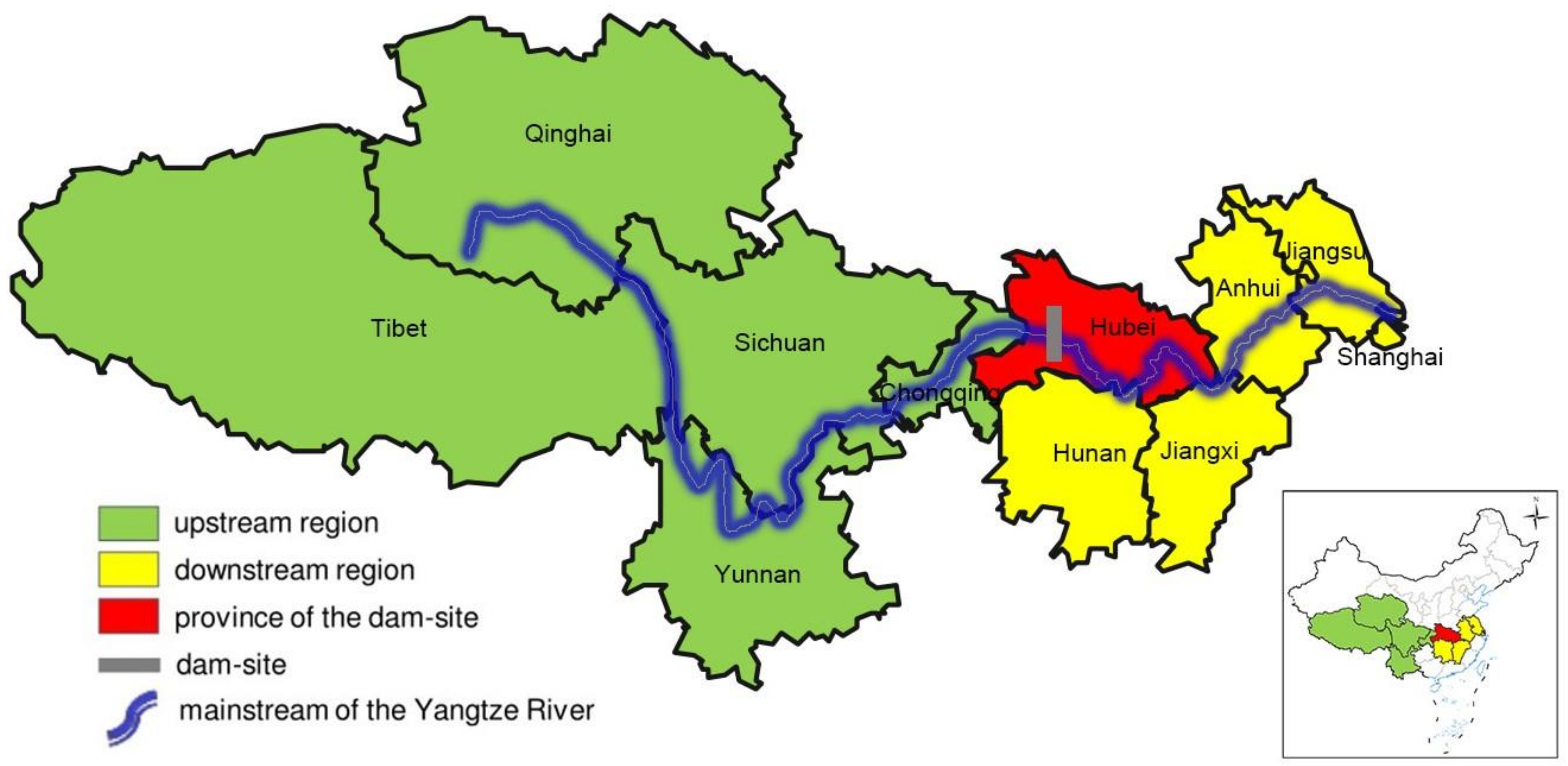
Regarding the sample selection, regions across and/or along the mainstream of the Yangtze River are regarded as the treatment group in this study, and the counties belong to the Yangtze River regions (Yangtze River regions include the provinces of Tibet, Qinghai, Sichuan, Yunnan, Chongqing, Hubei, Hunan, Jiangxi, Anhui, Jiangsu and Shanghai.) but not across the river are the control group. Counties along the main stream are selected as they experienced the exact same event, dammed and affected by the TGD since the year 1997, but they have various distances to the dam site. Notably, the control group is not directly affected by the TGD, but they are located at the neighborhood of the treatment group. On this basis, there exist 90 samples in the treatment group, and 661 counties in the control group. Figure 1 shows the distribution of the selected sample along the Yangtze River. The grey cutoff suggests the location of the dam site in Hubei province. The treatment group is exactly across or along the main stream.

Figure 1.
Map of the Yangtze River area and the TGD. Note: The base image for this map is from https://datav.aliyun.com/portal/school/atlas/area_selector (accessed on 26 May 2022).
In addition to county selection, distance to the dam site is another key variable of interest, but unfortunately, there are no existing data which provide the distance of each county to the dam site. Hence, it was necessary to collect this information personally. Specifically, the distances were calculated by using software to record how far away of each selected county is to the dam site. One issue of concern here is that distance to the dam site for the treatment group is not a simple straight line; instead, it is calculated exactly from the nearest boundary of a county to the dam site along the shape of the river, which should be longer than a straight line as the river is curved. For counties in the control group, as the distance according to the above description does not exist, the distances for each of them are obtained by calculating the average values of the treatment group of the same province. Samples are classified into three types according to their geographical locations: upstream, dam site (there is only one county just located at the dam site, which has zero distance to the dam), and downstream counties.
Descriptions of the main variables are given in Table 1, while Table 2, Table 3, Table 4 and Table 5 report statistical analysis of both the treatment group and control group. According to GDP growth, those tables indicate that counties along the Yangtze River were generally developing faster. However, the upstream areas are mostly located in the west of China, which were much less developed than the east, but the western counties are larger in area and faster in economic growth rate (recorded as 10.5% on average). Regarding agricultural records, it can be seen from Table 2, Table 3, Table 4 and Table 5 that the average yields of cotton and oil crops of the counties along the Yangtze River were on average higher than those of the neighboring counties. For the treatment group, the average yields of cotton and oil crops in the downstream regions of the Yangtze River were generally higher than those in the upstream regions.

Table 1.
Descriptions of the main variables.
Table 2.
Descriptive statistics of the main variables (treatment group).
Table 3.
Descriptive statistics of the main variables (control group).
Table 4.
More details of the treatment group (Average data values of the upstream, dam site and downstream).
Table 5.
More details of the treatment group (Average data values of different distances away from the dam site).
There is only one county which belongs to the dam site region, namely Yichang, with zero distance. In practice, the dam site has only one sample and it is very hard to run regressions; therefore, this observation is classified into the upstream group, as it has direct effects from the water falling down and accumulating at the reservoir. Additionally, the county Geermu in Qinghai province with the distance of 3958 km is the farthest sample away from the dam site, and it is also the headstream of the Yangtze River.
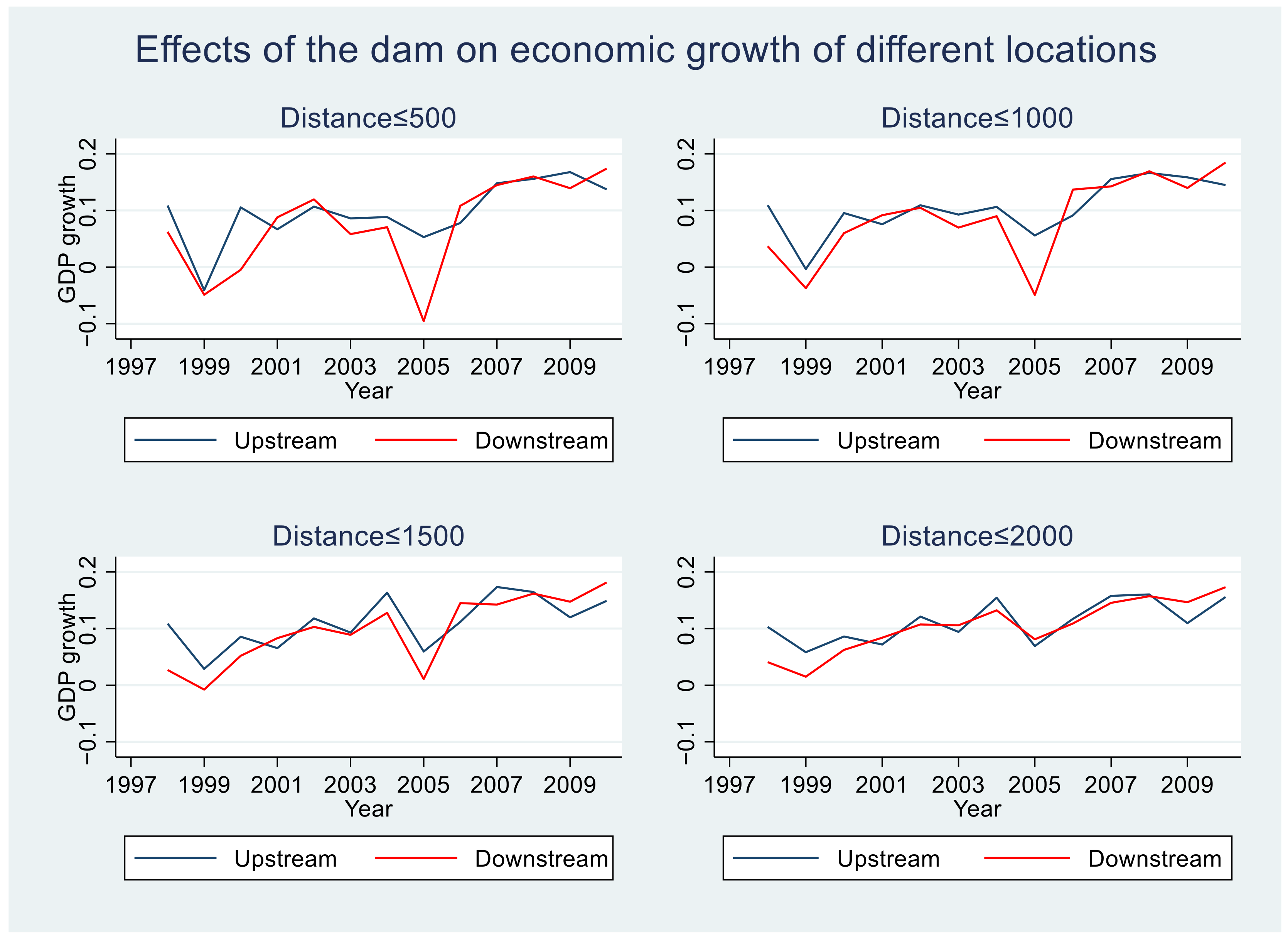
Figure 2 provides insights about the possible economic effects of the dam along the Yangtze River within 500 km/1000 km/1500 km/2000 km away from the dam site. By just focusing on the treatment group, samples closer to the dam site in the downstream area is with slower GDP comparing to the upstream counties. In the year 2005, both of the downstream and upstream regions have a declining trend especially for the counties within the distance of 500 km. However, this is not always the case; the GDP growth of the downstream region tends to exceed the upstream group after 2009, when the TGD project was completed.
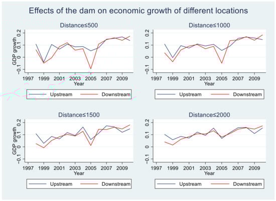
Figure 2.
Effects of the damming on the GDP growth of cotton production for upstream and downstream counties. Note: the unit of the distance in each graph is km.
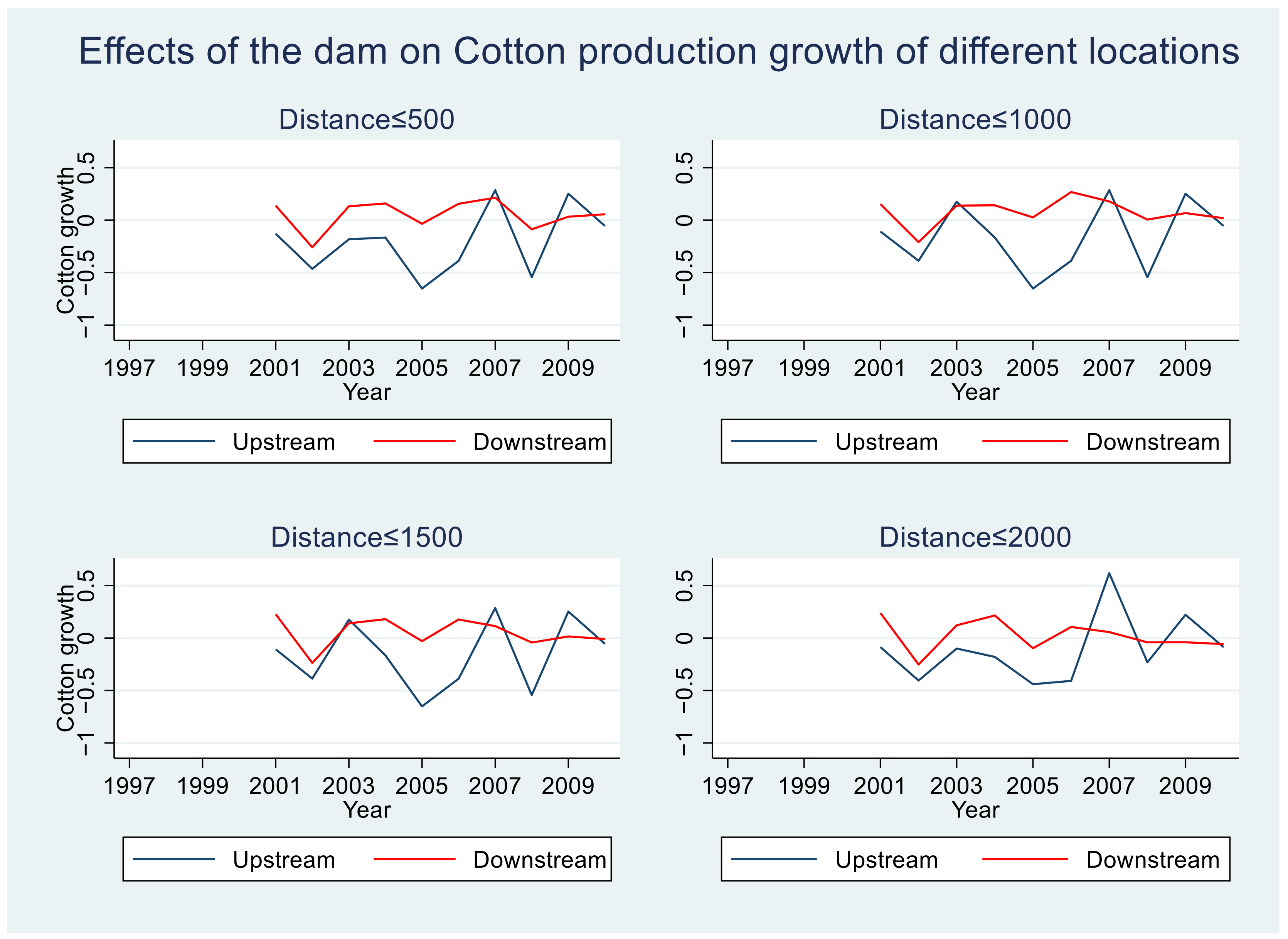
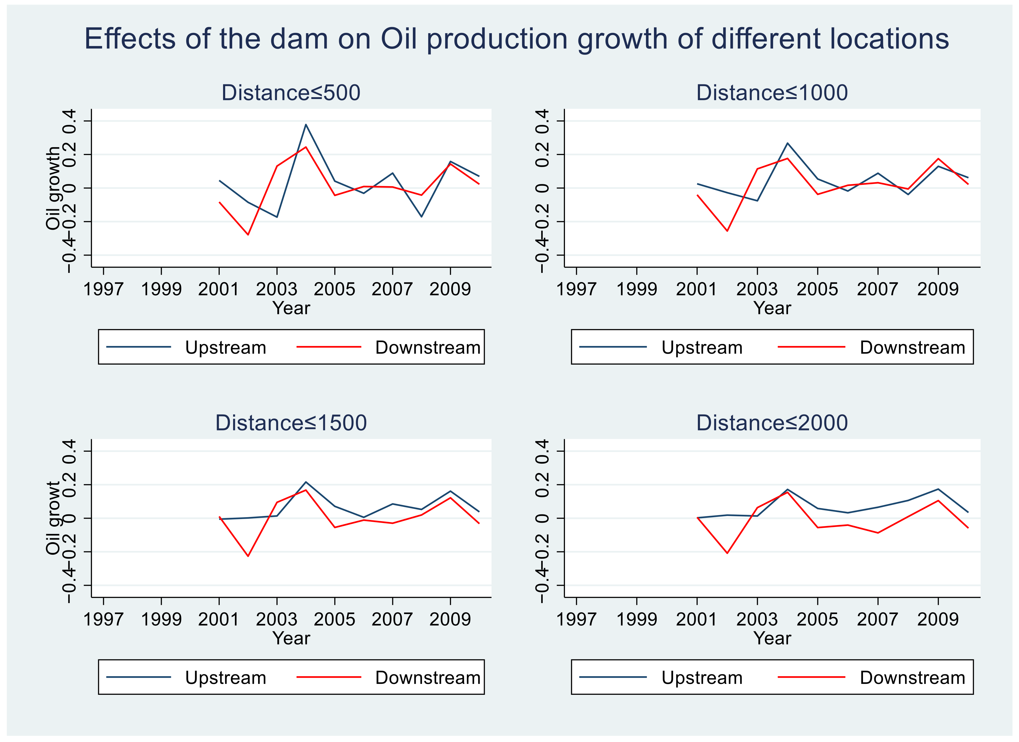
Figure 3 and Figure 4 illustrate the effects of the dam on cotton yield growth and oil yield growth, respectively. It can be seen from the two figures that the growth rate of the cotton production by different distances between the county and the dam site was generally faster in the downstream regions comparing to the upstream ones. However, the growth of oil yields was faster in the upstream regions. Due to the different situations for different crops, the agricultural impacts of building the TGD could also turn out to be different for different locations.
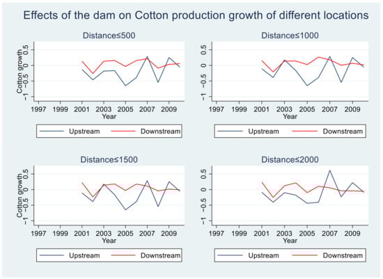
Figure 3.
Effects of the damming on the growth rate of cotton production for upstream and downstream counties. Note: the unit of the distance in each graph is km.
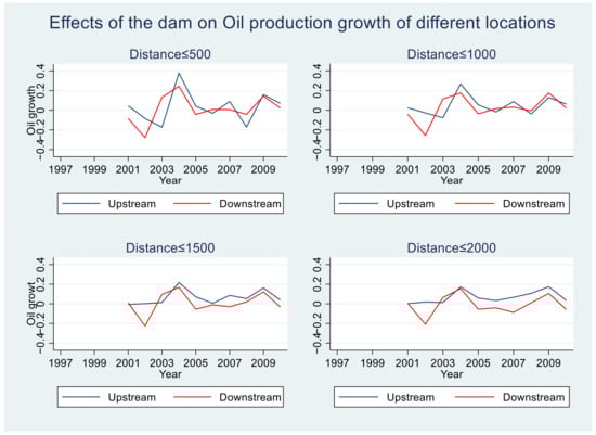
Figure 4.
Effects of the damming on the growth rate of oil production for upstream and downstream counties. Note: the unit of the distance in each graph is km.
3.2. Methodology
This article selects the counties along the Yangtze River as the treatment group, and the Yangtze River areas are the control group (see the distribution in Figure 1). The natural experience of the TGD cut the Yangtze River and brought enormous changes along the river. Before damming, the GDP, agricultural production and the county-level characteristics of the selected counties are well-recorded. After damming, counties along the river are directly affected by the shock, while those in the control group with similar characteristics were not affected by the TGD.
The methodology in use is Treatment Effect for Treated. Where Yi1(0) is the GDP per capita/agricultural production of county i in the treatment group in the basic year: 1997. Yi1t(1) represents the same issue of county i in the treatment group in year t (where t is from 1998 to 2010 according to the dataset). Similarly, we can obtain Yi0(0) and Yi0t(1) for the control group before and after the damming process. The causal effect is measured by calculating the different outcomes between the two groups, which is expressed as follows:
There are three variables of interest: the ‘river distance’, a dummy variable for whether the county is along the river, and a dummy variable for upstream location. Counties along the river are supposed to be directly affected by the TGD, and counties closer to the dam site naturally receive more direct impacts from the dam than those further away, and the upstream and downstream regions have some differences as well according to the biological/geographical characteristics of the dam system. Based on the previous analysis, the initial model is written as follows:
In Equation (2), dYit is the difference of GDP per capita of year j and the year 1997. Similarly, in order to examine the agricultural effect of the TGD, dYit also serves as the records of a certain sort of agricultural production in year j. On the right-hand side, di represents for ‘distance’. Ui is a dummy variable and equals to 1 if a sample located in the upstream of the dam site. Ri equals to 1 if the county is along the river. Zit represent some other control variables, for instance the provincial fixed effects and county-level characteristics. Tt is the year effect. This equation can be rewritten as Equation (3):
is the natural logarithm term of Yit for the county i at year t. Subtracting terms with and , we get Equation (4):
where is the error term, which mainly expains the differences in time and some other unobserved factors. symbolizes the intercept term. (where l = 1,2,3,4) are parameters of interest, which suggest the underlying effects of the TGD project during the process of construction. In our model, the ’Hausman test’ turns out to reject the random effect at the p-value of 0.078. This suggests the fixed effect is more appropriate.
This basic model is extended in mainly two steps: first, instead of adding the simple year term and the square term of the year, we multiple the dummy variables of each year from 1998 to 2010 with the term of ‘’ in Equation (4), and a series of intersection terms are obtained in the form of ‘’. This term gives more information on how the establishing periods and distance of each county dynamically contribute to GDP per capita, cotton yield and oil yield, respectively (see Equation (5)).
By classifying the years into four periods according to the official processes during the TGD construction, dummy variables of the periods are added in the model to clarify the effects of the TGD in various construction processes. The first period is the year 1997, and the next period is from 1998 to 2003, which begins with the damming year and ends with the official operation year. The third period is from 2004 to 2009. Finally, in the year 2010, the dam is well-finished and this period is regarded as the last step in our analysis.
Furthermore, by separating the samples a certain distance away from the dam (e.g., farther than 1000 km and less than 1000 km), it is a robust check to explore the effects of building the TGD. Equation (6) is accordingly given as below and it just includes the treatment group:
The above analysis only focuses on the damming shock in 1997, but this not the only shock within the 14 years. Another issue happened in 2003, which suggests the end of damming and the start of operation. Hence, the following model is accordingly established shown in Equation (7):
where the dummy variable Year03 suggests the shock took place in the year 2003, and it takes the value of 1 if the year equals to 2003 or afterwards.
4. Empirical Results
4.1. The Baseline Results
This part shows the baseline results based on Equation (4). Table 6 reports the estimated results for the basic model. The dependent variable represents the logarithm term of GDP per capita. It is clear that upstream counties averagely experienced significant positive effects on economic output comparing with downstream counties; the results show that the per capita GDP of the upstream counties increased by 14%. Building the TGD reduced the GDP per capita of the counties along the Yangtze River by 4.5%. By just observing the term ‘d*River’, generally, counties along the Yangtze River an additional 1 km further away from the dam site showed 0.006% less damage by the TGD. By exploring the effect of the interaction term ‘d*U’, the empirical results show that with 1 km distance away from the dam site, counties in the upstream region had a 0.02% increase in per capita GDP growth comparing to those in the downstream counties. Time effects are always positive as expected, which suggests the economy is growing with time.
Table 6.
Baseline results—the economic impact of building the TGD.
Table 7 reports the estimated results based on the basic model of Equation (4). As can be seen from Table 7, cotton production of the upstream counties was negatively affected by the damming. Additionally, the adverse effect is smaller if a county from the upstream is located further away from the dam site. In Column (3), oil crops along the upstream of the Yangtze River had a positive effect on its yield with 10% level of significance. Meanwhile, the yields of cotton and oil in the counties along the Yangtze River increased by 29.2% and 16.8% on average, respectively.
Table 7.
Baseline results—the agricultural impact of building the TGD.
The reason for the negative effect of building the TGD on cotton yield for the upstream region could be that: first, the upstream regions of the Yangtze River are not the main cotton planting areas, and hence the endowments for planting cotton are worse comparing with the downstream regions, such as the Jianghan plain and the Jianghuai Plain. The damming shock was likely to further damage the cultivated land in the upstream reservoir area, which contributed to the adverse effect on cotton yield. In contrast, the natural and socio-economic conditions of agricultural development in the downstream region are advantageous and suitable for large-scale cotton cultivation. The results also confirmed that the construction of the TGD accumulated more favorable conditions for cotton cultivation in downstream areas. Indeed, as the conditions for growing crops along the Yangtze River are favorable, the results confirmed that the cotton and oil crops in the counties along the Yangtze River were positively affected by building the dam.
According to Equation (5), Table 8 adds a series of intercept terms of the year dummy variable multiple by distance and the upstream dummy variable. Beside the same results obtained before, i.e., the upstream term was positive and the intercept term ‘d*U’ was negative, it is clear to observe that the intercept terms ‘Yearj*d*U’ turned out to be positive on GDP per capita (the parameters for each year of the ‘Yearj*d*U’ are not listed in Table 8; instead, they are described by a simple ‘POSITIVE’). The above outcomes are interesting in terms of illustrating that counties located far away earned long-lasting benefits in economic development with time. In other words, the dam negatively affects those regions closer to it.
Table 8.
Results estimating the extended model (dependent variable is ).
It is also important to examine the effects of damming by just keeping the treatment group and separating it into different groups of distance, such as 500 km/1000 km/1500 km. The relevant figures and estimated results are shown in the Appendix (see Figure A1/Table A1/Table A2 in Appendix A). Figure A1 indicates that counties closer to the dam site (within the distance of 500 km/1000 km/1500 km) generally had lower GDP per capita than those far away. According to this figure, there was a sudden decline after the TGD project began construction. However, a different phenomenon is observed in the last graph, which separates counties by the distance of within 2000 km and above 2000 km. Counties with shorter distances did not show poorer economic performance. There are mainly two reasons for this: one is that only a few samples are above 2000 km from the dam site, and those which are above 2000 km include a couple of the least developed counties in Qinghai and Tibet provinces; hence, they are likely to reduce the average level for economic items of the ‘≥2000 km’ group. Another reason is that the influence of the TGD is possibly limited within the threshold of 2000 km. Consequently, in empirical results, samples are only separated by 500 km, 1000 km and 1500 km, respectively. The main results of Table A1 are consistent with the results of the baseline table.
4.2. Robustness Checks
Table A1 shows that when the treatment sample is divided by the distance of 500 km, the results are more stable and significant than larger distance thresholds, which suggests that the dam site generated greater impacts on counties closer to it. The ‘distance’ term is negative, and the square of the distance is positive in the regressions of within 500 km. These suggested that within 500 km, the relationship between distance of the counties from the dam site and economic development was a U-shape, which decreased first, and then increased when the ‘distance’ grows.
From the results, it is clear to see that the term ‘d*U’ is significantly negative, the upstream term is positive and the downstream is negative. Those terms also suggested that the downstream areas were negatively affected by the dam building, which is also consistent with the expectation that after building the TGD, the downstream lakes would be drained and the water pollution would become worse.
Interestingly, in the downstream regression of within 500 km distance in Table A2, there is one unexpected term: ‘d*Down’. It turns out to be negative, which suggested that the counties located nearer the dam site in the downstream by an extra 1 km would increase 0.08% GDP per capita. In this situation, the possible benefits of the TGD was that it protects the downstream counties that are closer to the dam site from the flood, which were easily destroyed by the floods especially during the rainy season before damming; after damming, they had a higher chance to escape from terrible disasters.
Another important issue of the TGD occurred in 2003, when the dam began to function well. Before that, the dam was just under the process of building and the most important change caused by the project was damming and the rising water level; but after June 2003, the dam began to realize part of its functions, such as generating electricity. In this case, GDP is assumed to be stimulated by providing electricity power to big factories and millions of households in China. Furthermore, there are other effects such as migration and environmental issues that have indirect impacts on the economy and direct impacts on agricultural output.
In order to test for the exact impacts of the dam and compare the results of before and after its operation, another dummy variable ‘Year2003’ is added in the empirical model. It equals to 1 if the year is 2003 or afterward, and it equals to 0 before 2003. In the estimated model, some other intercept terms are created after adding this dummy variable. Table 9 shows the results.
Table 9.
Robust results—economic impact of building the TGD by setting 2003 as the basis year.
From Table 9, the term ‘Year03’ negatively affects the GDP per capita. This table also shows that the upstream region received economic benefit as the parameter before the term of upstream is positive as before. The intercept term ‘d*U* Year03’ was −0.007% for the upstream region, which showed that counties further away from the dam site after the year 2003 were negative. Furthermore, both of the columns suggested that counties located along the river with further distance had less been hurt in economic growth than the closer ones.
After adding some other control variables, similar results are obtained. Consequently, both the terms ‘*Year03* d’ and ‘Year03*River*d’ turned out to be significantly positive at the 1% level, which exactly reinforced the previous results that the treatment group with longer distances away from the dam were less hurt.
Regarding the results for agricultural productions, by taking 2003 as the shock year, the estimated results in Table 10 were similar to the baseline results in Table 7. From Table 10, the term ‘Year03’ had significantly positive effects on cotton and oil yields. The intercept terms ‘Year03*d’ in these four columns were significantly negative, indicating that crops planted farther away from the dam were less affected by damming in 2003. However, the terms ‘*Year03* d*U’ in the columns (1) and (2) were significantly negative, and in the columns (3) and (4) were significantly positive. Those results further confirmed that the operation of TGD enhanced functions of water storage, power generation, and flood control. Cotton production in the upstream regions remained significantly negative, indicating the construction of the TGD had a negative impact on cotton cultivation in the upstream regions. However, the impact of the TGD on oil yields was positively significant for the upstream regions. The results suggested that the functioning of the TGD provided rich water and favorable climate for oil cultivation in the upstream regions, and consequently promotes oil yields for the upstream river areas.
Table 10.
Robust results—agricultural impact of building the TGD by setting 2003 as the basis year.
5. Concluding Remarks
This paper provided empirical evidence to evaluate the economic and agricultural effects of the Three-Gorges Dam during the building period towards the counties along the main stream of the Yangtze River. The research was conducted by selecting 90 counties along/across the river and 661 counties located in the river areas for 14 years (from the start year of damming in 1997 to its finish in 2010). According to the previous literature, there are a wide variety of advantages and disadvantages both in the upstream and downstream regions of the dam site, and it is not possible to make a simple conclusion on which parts take the dominant position. This work dynamically evaluated and examined the economic and agricultural impacts by applying the ‘Treatment Effect for Treated method’ and comparing the samples in different locations, with different distances and in different periods of time. The results suggest that the short term after damming the TGD did not show any stable improvement in economy, especially as the counties geographically closer to the dam site in the downstream were generally negatively affected by the shock of damming (in the year 1997) and operation (in the year 2003). Regarding its impacts on cotton and oil yields, the results of the two crops turned out to be different. It showed a negative effect on cotton yield in the upstream regions, whereas there was a positive effect on oil yields for the same regions, especially since the operation of the TGD in 2003.
In particular, by recording the data of 14 years, on average, the upstream counties had priority to the downstream ones in GDP per capita and cotton planting. The results suggested that claims of protection from flood disasters were unable to exceed damages in particular regions. For instance, environmental pollution, emigration and drying lakes during the damming period occurred in the downstream regions. The estimated results also show the ‘winners’ and ‘losers’ in economic impact and various crop yields caused by damming, although the results were much more complex than simply an obvious conclusion. Counties with 1 km closer to the dam site in the upstream on average raised GDP per capita by 0.02%. This is in line with the phenomena that the dam site in the upstream areas stimulated the transportation and travel industries. On the contrary, the downstream lakes tended to be dried-up after damming. It also brought different impacts on crop cultivation, as the TGD directly affected water and land resources in the upstream and downstream regions, which affected the growth environment of crops. Based on their different growing needs, the TGD turned out to have different impacts on different crops.
The findings of this paper are important, as they give a detailed systemic evaluation of the TGD project for the first time. The findings illustrate the distribution of the various positive/negative effects caused by the dam in different periods of building. Furthermore, they have significant political implications: first, the analysis guides the government to compensate the counties near the downstream of the dam site by providing them economic compensation. Second, the results suggested that some of the functions such as irrigation and flood defense did not outweigh the losses of the counties in the downstream areas close to the dam site. Additionally, different crops are grown in different environments, and specific policies could be formulated for each type of crop in dealing with the adversely affected yields by damming. Some other practical actions could be taken based on the results of this paper. For instance, the government can instruct famers to apply advanced technologies and provide them subsidies for painting crops in particular regions along the river.
The DID analysis in this paper indicates the direction of follow-up research, such as exploring which channels result in the economic/agricultural outputs. Furthermore, this paper investigates that crop production is differently affected by the dam in different building periods. However, it remains unclear the exact reasons/channels of different impacts on different crops; for example, whether it is caused by water resources, land shrinkage or productivity decline. Due to the unavailability of these specific data, such as temperature, precipitation and sunshine duration, we cannot further analyze the specific reasons for the variation in cotton and oil crop productions, and these investigations are directions of the further research. Regarding the methodology in use, future research can also use machine learning and satellite data for in-depth analysis on this topic.
Author Contributions
Conceptualization, J.L.; methodology, J.L.; software, J.L. and L.L.; validation, J.L. and X.D.; formal analysis, J.L. and L.L.; investigation, J.L. and L.L.; resources, J.L. and X.D.; data curation, J.L. and L.L.; writing—original draft preparation, J.L. and L.L.; writing—review and editing, J.L., L.L. and X.D.; supervision, X.D.; project administration, J.L. and X.D.; funding acquisition, J.L. and X.D. All authors have read and agreed to the published version of the manuscript.
Funding
This research is supported by the National Natural Science Foundation of China (Grant No. 72104166), Ministry of Education of China, Youth Foundation Project of Humanities and Social Sciences (Grant No. 19YJC790059), Philosophy and Social Science Research Planning Project in Chengdu–Chengdu Urban Fringe Development and Co-coordinating Urban and Rural (Grant No. CXRH2022YB03), Sichuan Research Centre on the Mountainous Ethnic Minority Regional Economic Development (Grant No. SDJJ202101), Sichuan Center for Rural Development Research (Grant No. CR2110).
Institutional Review Board Statement
Not applicable.
Informed Consent Statement
Not applicable.
Data Availability Statement
The dataset generated and/or analyzed during the present study is available from the corresponding author.
Conflicts of Interest
The authors declare no conflict of interest.
Appendix A
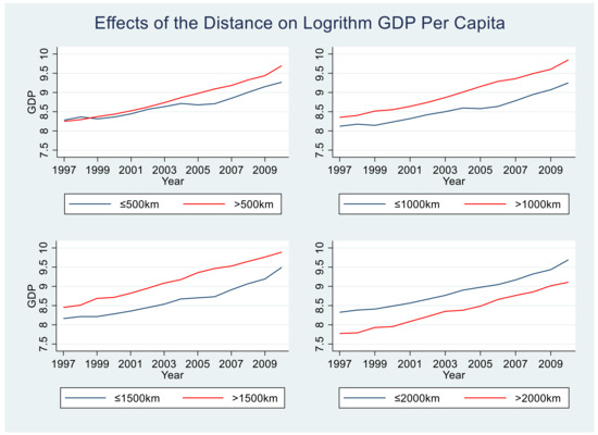
Figure A1.
Relationships between distance and GDP.
Figure A1.
Relationships between distance and GDP.
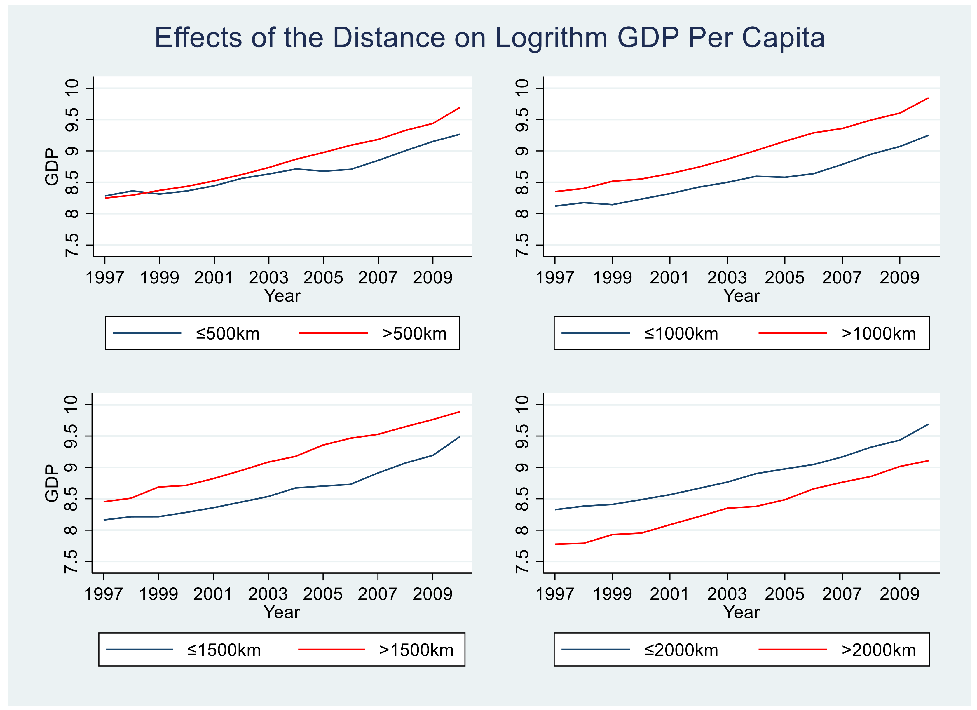
Table A1.
The robust results—The economic impact of building the TGD by different groups of distance (The upstream regions).
Table A1.
The robust results—The economic impact of building the TGD by different groups of distance (The upstream regions).
| Variable | ≤500 km | ≤1000 km | ≤1500 km |
|---|---|---|---|
| U | 0.685 ** | 0.770 *** | 0.283 *** |
| (0.294) | (0.252) | (0.161) | |
| d | −0.003 * | 0.001 | 0.0005 * |
| (0.0018) | (0.0007) | (0.0003) | |
| d2 | 5.95 × 10⁶ ** | −7.02 × 10⁻⁷ | −3.43 × 10⁻⁷ |
| (2.97 × 10⁻⁶) | (7.39 × 10⁻⁷) | (2.47 × 10⁻⁷) | |
| d*U | −0.00005 | −0.0006 * | −0.0003 |
| (0.0008) | (0.0003) | (0.0004) | |
| Year | 0.035 *** | 0.042 *** | 0.046 *** |
| (0.009) | (0.007) | (0.006) | |
| Year2 | 0.001 | 0.004 *** | 0.004 *** |
| (0.0007) | (0.0006) | (0.0005) | |
| Power spread | −0.089 *** | −0.165 *** | −0.203 *** |
| (0.032) | (0.025) | (0.021) | |
| Direct administration | 0.120 *** | 0.102 ** | 0.086 ** |
| (0.039) | (0.042) | (0.043) | |
| Area | −0.015 ** | −0.012 *** | −0.002 * |
| (0.006) | (0.004) | (0.001) | |
| Lgdp_ pre | 0.105 *** | 0.143 *** | 0.114 *** |
| (0.029) | (0.022) | (0.016) | |
| Lgagri | 0.554 *** | 0.072 | 0.067 |
| (0.084) | (0.054) | (0.043) | |
| Constant | −4.543 *** | −1.823 *** | −1.735 *** |
| (0.084) | (0.435) | (0.345) | |
| Province | YES | YES | YES |
| No. of group | 18 | 36 | 59 |
| Observations | 243 | 481 | 765 |
| R-squared | 0.83 | 0.71 | 0.77 |
Notes: The figures in the parentheses are standard errors; *** denotes significance at the 1% level; ** denotes significance at the 5% level; * denotes significance at the 10% level. The dummy variables ‘Province’ are provincial fix effects.
Table A2.
The robust results—The economic impact of building the TGD by different groups of distance (The downstream regions).
Table A2.
The robust results—The economic impact of building the TGD by different groups of distance (The downstream regions).
| Variable | ≤500 km | ≤1000 km | ≤1500 km |
|---|---|---|---|
| Down | 0.108 | 0.073 | −0.127 * |
| (0.146) | (0.094) | (0.067) | |
| d | −0.004 *** | −0.0001 | −0.0001 |
| (0.0008) | (0.0002) | (0.0002) | |
| d2 | 8.22 × 10⁻⁶ *** | 1.16 × 10⁻⁷ | 1.71 × 10⁻⁷ * |
| (1.41 × 10⁻⁶) | (2.52 × 10⁻⁷) | (9.79 × 10⁻⁸) | |
| d*Down | −0.0008 ** | 0.0001 | −0.0001 |
| (0.00038) | (0.0001) | (0.0002) | |
| Year | 0.069 *** | 0.119 *** | 0.131 *** |
| (0.013) | (0.011) | (0.010) | |
| Year2 | −0.003 *** | −0.005 *** | −0.005 *** |
| (0.001) | (0.001) | (0.0008) | |
| Power spread | −0.022 | −0.106 *** | −0.139 *** |
| (0.046) | (0.039) | (0.034) | |
| Direct administration | 0.131 ** | -0.035 | 0.086 ** |
| (0.053) | (0.052) | (0.043) | |
| Area | −0.004 | 0.001 | −0.001 |
| (0.003) | (0.0015) | (0.061) | |
| Lgdp_pre | 0.353 *** | 0.553 *** | 0.542 *** |
| (0.037) | (0.029) | (0.021) | |
| Lgagri | 0.604 *** | 0.384 *** | 0.330 *** |
| (0.082) | (0.052) | (0.042) | |
| Constant | 1.350 ** | 0.544 * | 1.314 *** |
| (0.649) | (0.318) | (0.292) | |
| Province | YES | YES | YES |
| No. of group | 18 | 37 | 61 |
| Observations | 243 | 481 | 781 |
| R-squared | 0.87 | 0.82 | 0.86 |
Notes: The figures in the parentheses are standard errors; *** denotes significance at the 1% level; ** denotes significance at the 5% level; * denotes significance at the 10% level; The dummy variables ‘Province’ are provincial fixed effects.
References
- McCully, P. Silenced Rivers: The Ecology and Politics of Large Dams; Zed Books: London, UK, 2001. [Google Scholar]
- Renofalt, B.M.; Jansson, R.; Nilsson, C. Effects of hydropower generation and opportunities for environmental flow management in Swedish riverine ecosystems. Freshw. Biol. 2010, 55, 49–67. [Google Scholar] [CrossRef]
- Pan, B.; Yuan, J.; Zhang, X.; Wang, Z.; Chen, J.; Lu, J.; Yang, W.; Li, Z.; Zhao, N.; Xu, M. A review of ecological restoration techniques in fluvial rivers. Int. J. Sediment Res. 2016, 31, 110–119. [Google Scholar] [CrossRef]
- Hudson, P.F.; van der Hout, E.; Verdaasdonk, M. (Re)Development of fluvial islands along the lower Mississippi River over five decades, 1965–2015. Geomorphology 2019, 331, 78–91. [Google Scholar] [CrossRef]
- Chen, X.; Zhu, Q.; Yang, Z.; Sun, H.; Zhao, N.; Ni, J. Filtering Effect of Rhinogobio cylindricus Gut Microbiota Relieved Influence of the Three Gorges Dam on the Gut Microbiota Composition. Water 2021, 13, 2697. [Google Scholar] [CrossRef]
- Shen, Y.; Cheng, R.; Xiao, W.; Zeng, L.; Wang, L.; Sun, P.; Chen, T. Temporal dynamics of soil nutrients in the riparian zone: Effects of water fluctuations after construction of the Three Gorges Dam. Ecol. Indic. 2022, 139, 108865. [Google Scholar] [CrossRef]
- Ren, Q.; Li, C.; Yang, W.; Song, H.; Ma, P.; Wang, C.; Schneider, R.L.; Morreale, S.J. Revegetation of the riparian zone of the Three Gorges Dam Reservoir leads to increased soil bacterial diversity. Environ. Sci. Pollut. Res. 2018, 25, 23748–23763. [Google Scholar] [CrossRef] [PubMed]
- Ren, Q.; Song, H.; Yuan, Z.; Ni, X.; Li, C. Changes in Soil Enzyme Activities and Microbial Biomass after Revegetation in the Three Gorges Reservoir, China. Forests 2018, 9, 249. [Google Scholar] [CrossRef]
- Elisabeth, M.P.; George, T. Risk Costs for New Dams: Economic Analysis and Effects of Monitoring. Water Resour. Res. 1986, 22, 5–14. [Google Scholar]
- Dai, Z.; Liu, J.T. Impacts of large dams on downstream fluvial sedimentation: An example of the Three Gorges Dam (TGD) on the Changjiang (Yangtze River). J. Hydrol. 2013, 480, 10–18. [Google Scholar] [CrossRef]
- Jackon, S.; Sleigh, A. Resettlement for China’s Three Gorges Dam: Socio-economic impact and institutional tensions. Communist Post-Communist Stud. 2000, 33, 223–241. [Google Scholar] [CrossRef]
- Wu, J.; Huang, J.; Han, X.; Xie, Z.; Gao, X. Three-Gorges Dam—Experiment in Habitat Fragmentations? Science 2003, 300, 1239–1240. [Google Scholar] [CrossRef]
- Yang, Y.; Chen, T.; Liu, X.; Wang, S.; Wang, K.; Xiao, R.; Chen, X.; Zhang, T. Ecological risk assessment and environment carrying capacity of soil pesticide residues in vegetable ecosystem in the Three Gorges Reservoir Area. J. Hazard. Mater. 2022, 435, 128987. [Google Scholar] [CrossRef]
- Huang, C.; Zhao, D.; Deng, L. Landscape pattern simulation for ecosystem service value regulation of Three Gorges Reservoir Area, China. Environ. Impact Assess. Rev. 2022, 95, 106798. [Google Scholar] [CrossRef]
- Guo, H.; Hu, Q.; Zhang, Q.; Feng, S. Effects of the Three Gorges Dam on Yangtze River flow and river interaction with Poyang Lake, China: 2003-2008. J. Hydrol. 2012, 416–417, 19–27. [Google Scholar] [CrossRef]
- Shankman, D.; Liang, Q. Landscape changes and increasing flood frequency in China’s Poyang Lake region. Prof. Geogr. 2003, 55, 434–445. [Google Scholar] [CrossRef]
- Shankman, D.; Keim, B.D.; Song, J. Flood frequency in China’s Poyang Lake region: Trends and teleconnections. Int. J. Climatol. 2006, 26, 1255–1266. [Google Scholar] [CrossRef]
- Duflo, E.; Pande, R. Dams; Working Paper; NBER: Cambridge, MA, USA, 2005. [Google Scholar]
- Yang, Z.; Wang, H.; Saito, Y.; Milliman, J.D.; Xu, K.; Qiao, S.; Shi, G. Dam impacts on the Changjiang (Yangtze) River sediment discharge to the sea: The past 55 years and after the Three Gorges Dam. Water Resour. Res. 2006, 42, W04407. [Google Scholar] [CrossRef]
- Zhu, Z.; Zhao, K.; Lin, Q.; Salman, Q.; Cynthia, R.; Cai, G.; Wang, H. Systematic Environmental Impact Assessment for Non-natural Reserve Areas: A Case Study of the Chaishitan Water Conservancy Project on Land Use and Plant Diversity in Yunnan, China. Front. Ecol. Evol. 2017, 5, 60. [Google Scholar] [CrossRef]
- Zhai, M.; Huang, G.; Li, J.; Pan, X.; Su, S. Development of a distributive Three Gorges Project input-output model to investigate the disaggregated sectoral effects of Three Gorges Project. Sci. Total Environ. 2021, 797, 148817. [Google Scholar] [CrossRef]
- Bao, X. Dams and Intergovernmental Transfer: Are Dam Projects Pareto Improving in China? Working Paper; Columbia University: New York, NY, USA, 2012. [Google Scholar]
- Loomis, J. Measuring the economic benefits of removing dams and restoring the Elwha River: Results of a contingent valuation survey. Water Resour. Res. 1996, 32, 441–447. [Google Scholar] [CrossRef]
- Gelfenbaum, G.; Stevens, A.W.; Miller, I.; Warrick, J.A.; Ogston, A.S.; Eidam, E. Large-scale dam removal on the Elwha River, Washington, USA: Coastal geomorphic change. Geomorphology 2015, 246, 649–668. [Google Scholar] [CrossRef] [Green Version]
- Bohlen, C.; Lewis, L. Examining the economic impacts of hydropower dams on property values using GIS. J. Environ. Manag. 2009, 90, 258–269. [Google Scholar] [CrossRef] [PubMed]
- Borimnejad, V.; Salimian, F. Investigation of socio-economic and environmental effects of Taleghan dam using structural equation modeling. Int. J. Agric. Manag. Dev. 2014, 4, 193–202. [Google Scholar]
- Zhang, T.; Yang, Y.; Ni, J.; Xie, D. Construction of an integrated technology system for control agricultural non-point source pollution in the Three Gorges Reservoir Areas. Agric. Ecosyst. Environ. 2020, 295, 106919. [Google Scholar] [CrossRef]
- Xu, K.; Milliman, D.J. Seasonal variations of sediment discharge from the Yangtze River before and after impoundment of the Three Gorges Dam. Geomorphology 2009, 104, 276–283. [Google Scholar] [CrossRef]
- Müller, B.; Berg, M.; Yao, Z.; Zhang, X.; Wang, D.; Pfluger, A. How polluted is the Yangtze river? Water quality downstream from the Three Gorges Dam. Sci. Total Environ. 2008, 402, 232–247. [Google Scholar] [CrossRef]
- Liang, X.; Li, Y. Identification of spatial coupling between cultivated land functional transformation and settlements in Three Gorges Reservoir Area, China. Habitat Int. 2020, 104, 102236. [Google Scholar] [CrossRef]
- Nakayama, T.; Shankman, D. Impact of the Three-Gorges Dam and water transfer project on Changjiang floods. Glob. Planet. Chang. 2013, 100, 28–50. [Google Scholar] [CrossRef]
- Tian, Y.; Huang, Z.; Xiao, W. Reductions in non-point source pollution through different management practices for an agricultural watershed in the Three Gorges Reservoir Area. J. Environ. Sci. 2010, 22, 184–191. [Google Scholar] [CrossRef]
- Liang, X.; Li, Y.; Shao, J.; Ran, C. Traditional agroecosystem transition in mountainous area of Three Gorges Reservoir Area. J. Geogr. Sci. 2020, 30, 281–296. [Google Scholar] [CrossRef]
- Qian, N. Missing Women and the Price of Tea in China: The Effect of Sex-Specific Earnings on Sex Imbalance. Q. J. Econ. 2008, 123, 1251–1285. [Google Scholar] [CrossRef]
- Meng, L. Evaluating China’s poverty alleviation program: A regression discontinuity approach. J. Public Econ. 2013, 101, 1–11. [Google Scholar] [CrossRef]
- Chen, Y.; Ebenstein, A.; Greenstone, M.; Li, H. Evidence on the impact of sustained exposure to air pollution on life expectancy from China’s Huai River policy. Proc. Natl. Acad. Sci. USA 2013, 110, 12936–12941. [Google Scholar] [CrossRef] [PubMed]
- Deng, G.; Gan, L.; Hernandez, M.A. Do natural disasters cause an excessive fear of heights? Evidence from the Wenchuan earthquake. J. Urban Econ. 2015, 90, 79–89. [Google Scholar] [CrossRef] [PubMed]
Publisher’s Note: MDPI stays neutral with regard to jurisdictional claims in published maps and institutional affiliations. |
© 2022 by the authors. Licensee MDPI, Basel, Switzerland. This article is an open access article distributed under the terms and conditions of the Creative Commons Attribution (CC BY) license (https://creativecommons.org/licenses/by/4.0/).