Temporal and Spatial Positioning of Service Crops in Cereals Affects Yield and Weed Control

Abstract

Leguminous service crops (SCs) can provide multiple services to cropping systems, reducing the reliance on external resources if sufficient biomass is produced. However, rapid light and temperature reductions limit post-harvest cultivation of SCs in Northern Europe. A novel practice of intercropping SCs in two consecutive crops (spring–winter cereal) to extend the period of SCs growth, and hence improve yield and reduce weeds, was tested. Three spatial and temporal arrangements of SCs and cash crops were investigated, as well as three SC mixtures, characterized by their longevity and frost sensitivity. Compared to no SC, the best performing mixture, frost-tolerant annuals, increased grain and N yield of winter wheat by 10% and 19%, respectively, and reduced weed biomass by 15% and 26% in oats and winter wheat, respectively. These effects were attributed to high biomass production and winter survival. However, this SC reduced oat yields by 15% compared to no SC. Furthermore, SC growth and service provision varied largely between experiments, driven by the weather conditions. Extending the SC’s growth period by intercropping in two consecutive cereal crops has potential, but locally adapted species choices and establishment strategies are needed to ensure SC vitality until termination.

1. Introduction

Including legume crops as living ground cover can improve the performance of cropping systems by providing additional ecosystem services [1]. Among the services are, maintaining soil biological activity [2], suppressing weeds [3], protecting the soil from wind and water erosion [4], retaining nutrients [5,6], increasing soil organic carbon content [7], and the addition of nutrients via dinitrogen (N₂) fixation [8] or nutrient mining from deeper soil layers [9]. It has also been shown that several desired services can be provided simultaneously [10], indicating the great potential of using these crops as a tool for more sustainable agriculture. Crops that are managed as living ground cover may have different names, depending on their main function and how they are used in the cropping system [11]. In this paper, we use the term service crops (SCs) for these crops to emphasize that their role is to provide one or more services supporting the cropping system.

Biomass production has been shown to correlate well with several target functions of service crops, including ground cover, weed suppression, and reduced nitrate leaching [12], as well as the yield of the subsequent crop. For example, under northern European conditions, grass/clover under-sown into spring barley can produce about 2 t dry matter ha⁻¹ of biomass until late in autumn if conditions are suitable [13]. This led to a yield increase in subsequent spring barley by 1–2 t ha⁻¹ when the grass/clover crop had been ploughed under in late autumn. Similar amounts of service crop biomass have, in other studies in northern Europe, been shown to also reduce N leaching by about 70% [14]. Achieving sufficient service crop biomass can, however, be difficult in northern Europe if the service crop is sown after cash crop harvest due to low daily incoming solar radiation and temperatures [15], meaning that SCs are mainly used prior to a spring-sown cash crop. Spring-sown cash crops, however, generally yield lower than autumn sown cash crops, and when autumn tillage is required, as on clay soils, the soil will be left bare for several months. Bare soils are prone to erosion as well as weed infestation, and SCs grown during autumn–spring can serve an important role in reducing both [16,17]. Extending the growth period of SCs, their establishment as well as termination time, into periods when the cash crops are growing but not using all available resources is a potential way to increase their biomass production and the related services.

In intercropping, two or more species are grown together to have more efficient use of resources, compensate poor performance of the other species, and/or cooperate via modifications of the environment [18]. Intercropping the SCs with a cash crop can also have undesired consequences, sometimes called “disservices”. The most obvious and important for many farmers is competition between the SC and the cash crop, resulting in cash crop yield reduction [18,19]. However, it is possible to mitigate these undesired consequences to some extent through cropping system design and management [19]. Finding suitable combinations of cash crop and SC species according to the desired services, as well as designing the system to minimize competition with the cash crop, are clearly priorities and need to be done, taking local conditions into consideration. Understanding how to manage the different species to utilize resources in a complementary way in space and time is one of the keys to successful intercropping [18].

In this study, our aim was to evaluate how different functional groups of leguminous SCs affect cereal yield and weed biomass when intercropped in a spring oats-winter wheat cropping sequence under organic management. The SCs comprised three mixtures differing in longevity and frost sensitivity. This affected their period of main biomass production, which was either in summer or autumn/spring or continuously throughout the experimental period. Three spatial arrangements of the crops (SCs and cash crops) were also tested, with associated differences in SC growth and crop management.

We hypothesized that the SC mixtures, with their ability to fix atmospheric nitrogen and the additional biomass they provide, would (1) increase winter wheat grain yield, (2) suppress weeds, and (3) not jeopardize the yields of oats. The hypotheses were tested in four field experiments conducted in two regions of southern Sweden.

2. Materials and Methods

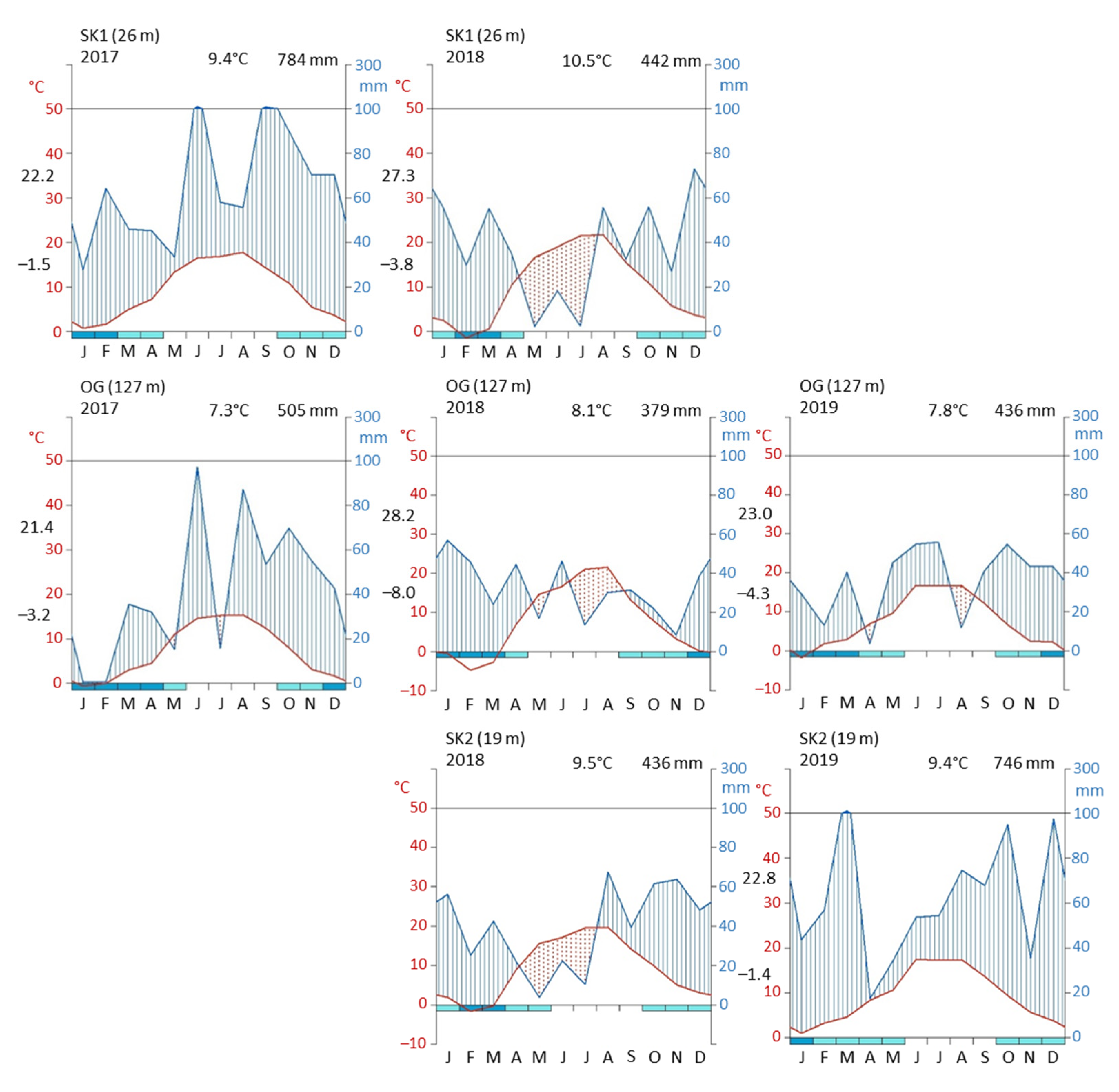
2.1. Experimental Sites

The four experiments were located on organic farms in two cereal-dominated regions of Sweden, the provinces Skåne (SK) and Östergötland (OG). In each region, two experiments were set up in 2017 (SK1, 55°40″ N 13°13″ E and OG1, 58°26″ N 15°18″ E) and 2018 (SK2, 56°13″ N 12°54″ E and OG2, 58°26″ N 15°18″ E). The 30-year means for annual temperatures are 9.0, 8.4, and 7.1 °C, and for annual precipitation are 676, 755, and 565 mm at SK1, SK2, and the two OG experimental sites, respectively. During the study, weather conditions differed much between experiments and years (Figure 1). Water surpluses were generally greater in SK than in OG, but precipitation was extremely low during summer at all sites in 2018.

The topsoil was classified as loam at SK1, clay loam at SK2, silty clay loam at OG1, and silty clay at OG2 (USDA, 2022), with a general increase in the finer particle sizes in the subsoil (Table S1.1). Topsoil pH (H₂O) ranged from 6.8 to 7.1 between sites and in the subsoil between 7.2 and 7.8. Soil mineral nitrogen was about 0.5 mg 100 g⁻¹ in the topsoil prior to the experiment’s start, except for SK2, where it was about half as much. Soil carbon was generally higher in the OG experiments than in the SK experiments (Table S1.1).

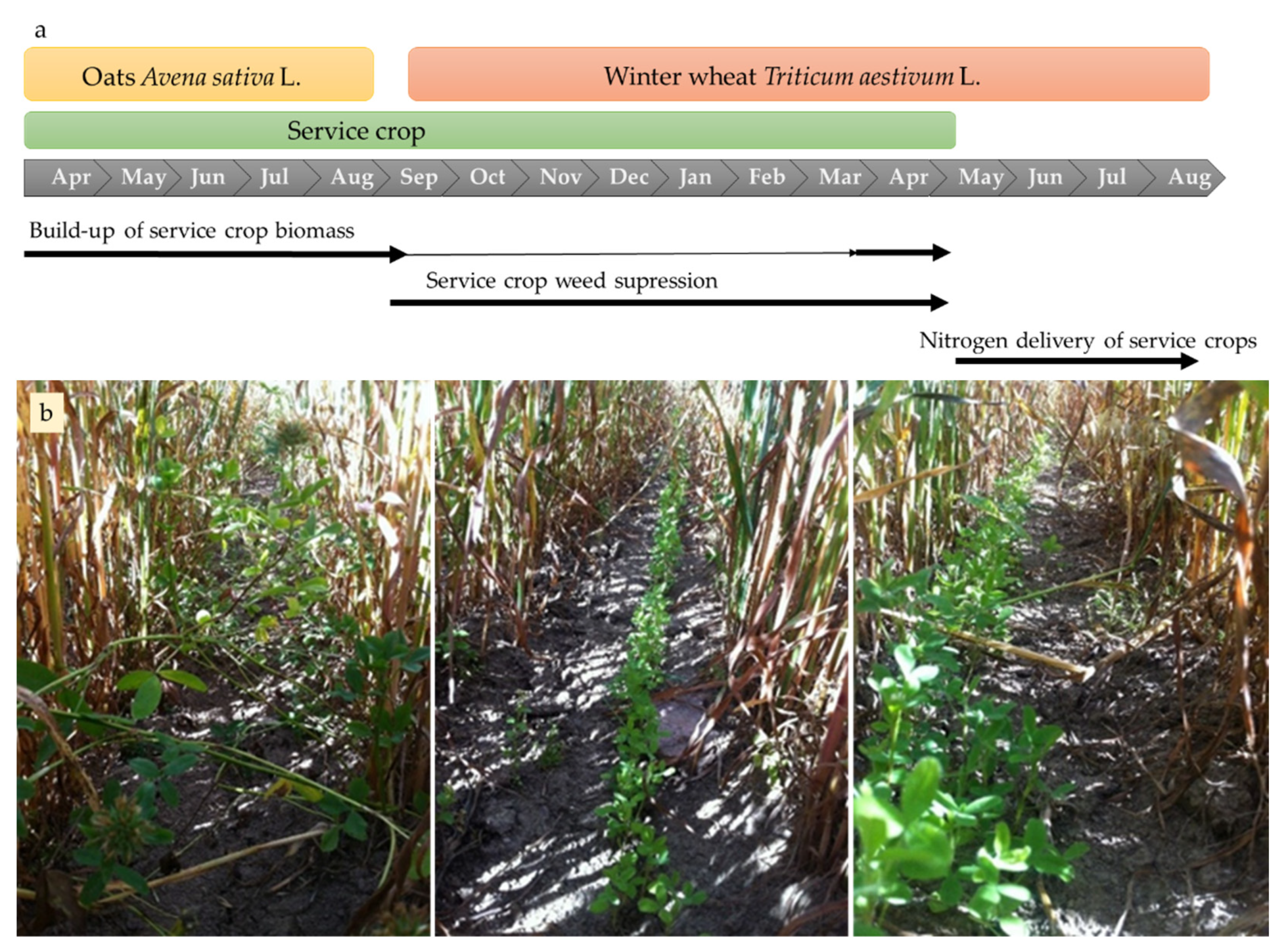
2.2. Crop Sequence and Management

The first cash crop was spring oats (Avena sativa L.), followed by direct-seeded winter wheat (Triticum aestivum L.). Service crops (SCs) were sown into oats and were intercropped with both oats and winter wheat until they were terminated in the spring of the second year (Figure 2a). Due to wet conditions in autumn 2017, it was not possible to sow winter wheat in experiment OG1. In this experiment, winter wheat was replaced with spring wheat, and therefore this experiment was excluded from the analyses in its second year, 2019.

The experiments in OG were conducted with experimental equipment in small plots, 3.1 m × 36 m, while the experiments in SK were managed by the farmers with their own machinery; hence, larger plot sizes were used (8 m and 9 m × 50 m in SK1 and SK2, respectively). The smaller plots in OG allowed for more treatments (see Section 2.3 for a detailed description), and a total of 9 treatments were included in the study. At SK, the experimental design was reduced to include only 6 treatments (

Table 1. Main characteristics of the different levels of the two treatment factors; service crop mixture and system strategy. The two columns to the far right indicate at which experimental regions, SK = Skåne or OG = Östergötland, each factor level is present. For visualization of the sowing of service crops in the different system strategies, see Figure 2b.

Service Crop Mixture	Speed of Growth	Frost Sensitivity		SK	OG
Frost-sensitive annual *	Fast	High		X	X
Perennial **	Slow	Low		X	X
Frost-tolerant annual ***	Fast	Relatively low			X
Control, no service crop				X	X
System strategy	Sowing of service crops	Number of row hoeing events	Sowing of winter wheat	SK	OG
Early Intra	Same time as oats, in oat rows	2	Between oat rows	X	X
Late Inter	At first row hoeing, in inter-row centers	1	In oat stubble	X	X
Late Adjacent	At first row hoeing, adjacent to oat row	2	Between oat rows		X

* Squarrose clover (Trifolium squarrosum) and Persian clover (T. resupinatum). ** Red clover (T. pratense), white clover (T. repens), and the short-lived perennial black medic (Medicago lupulina). *** Crimson clover (T. incarnatum) and hairy vetch (Vicia villosa).

). Oat was sown in 7 cm bands with inter-row distances of 33 cm in the OG experiments, 25 cm in experiment SK1, and 32 cm in experiment SK2 due to different machines. Winter wheat was direct drilled with straight coulters leaving approximately 2 cm-wide rows. For information on the timing of field operations, see Table S1.3.

2.3. Experimental Design

The two experimental factors, service crop mixture and system strategy (Table 1), were arranged in randomized complete blocks with four replicates (five at experiment OG2, for data from cash crop harvest). Six treatment combinations were tested in all experiments. In the OG experiments, there was one additional level for each factor, and hence twelve treatment combinations (Table 1).

2.3.1. Service Crop Mixtures

The SCs were grouped into mixtures according to the functional traits of frost sensitivity and longevity. The groups were (i) frost-sensitive annuals, which included squarrose clover (Trifolium squarrosum L.) and Persian clover (T. resupinatum), (ii) perennials, which included red clover (T. pratense), white clover (T. repens) and the short-lived perennial black medic (Medicago lupulina L.), and (iii) frost-tolerant annuals, which included crimson clover (T. incarnatum) and hairy vetch (Vicia villosa Roth). Frost-tolerant annual SCs were only present in the experiments in OG. Sowing density for annual SCs was 250 viable seeds m⁻² per species, except for V. villosa, which, due to its vigorous growth, was sown with 30 viable seeds m⁻², and for perennial species, the rates were 167 and 95 viable seeds m⁻² per species in the SK and OG experiments, respectively (Table S1.2). For each system strategy (see below), there was also control without SCs.

2.3.2. System Strategy

The system strategies differed in their spatial and temporal arrangement of cash crops and SCs (Figure 2b), which also affected row hoeing intensity (Table 1). In the first system strategy, Early Intra, SCs were sown at the same time and in the same rows as oats. The inter-row space in Early Intra was crop free during the whole oat cropping sequence and was hoed twice. Winter wheat was direct drilled in the inter-row space after oat harvest. In system strategies, Late SCs were sown between the rows of oat approximately one month after the sowing of oats. The sowing with both strategies was performed in conjunction with row hoeing. In Late Inter, the SCs were sown in oat inter-row centres, and the SCs, therefore, prevented later row hoeing. Winter wheat was direct drilled in the row of oat stubble. In Late Adjacent (only in the OG experiments), SCs were sown adjacent to the oat, thus allowing for a second-row hoeing if needed (not done), but with a smaller hoe than in Early Intra. Winter wheat was direct drilled into the inter-row space of SCs. In winter wheat, row hoeing was conducted twice with all system strategies.

2.4. Data Collection

Destructive sampling was restricted to the two ends of the experimental plots, saving the plot centre for crop harvest (Figure 3a). Sampling of SC and weed data was performed from an area covering two cash crop rows and two inter-row spaces (i.e., 50 cm or wider) and 50 cm long (Figure 3b). The different sizes of the areas were accounted for in later calculations. Samples from each frame were pooled into one sample per plot. For detailed timing of data collection, see Table S1.4.

2.4.1. Service Crop Performance

Service crop performance was evaluated by measures of (i) plant density, (ii) biomass production until oat harvest, (iii) autumn soil cover, and (iv) percent N derived from the atmosphere (%Ndfa). Data on SC performance were only collected from system strategies Early Intra and Late Inter. For all variables except %Ndfa, the data were collected according to the above description. Biomass was collected at the species level and cut at ground level when the cash crop approached maturity. Percent soil cover was assessed before winter. For the %Ndfa analysis, above-ground biomass was collected from 10 randomly selected plants from each SC species within each plot in late autumn. In 2017, SC samples were only collected from treatments with system strategy Late Inter because there was almost no biomass present in treatments with system strategy Early Intra. All biomass samples were dried at 60 °C for 48 h before weighing or further sample treatment (see below).

Nitrogen Isotope Analysis

Plants were thoroughly washed before drying. The dried plant samples were ball milled and analysed with an Elemental Analyzer (Flash EA 2000, Thermo Fisher Scientific, Bremen, Germany) and Isotope Ratio Mass Spectrometer (EA-IRMS, DeltaV, Thermo Fisher Scientific, Bremen, Germany) according to [21] for δ¹⁵N isotope profiles. Calibrated samples with wheat and maize flour were used as working standards.

The N₂ fixation of each SC species was estimated by calculating the percentage of N derived from the atmosphere (%Ndfa) according to [22]:

%Ndfa = (δ¹⁵N_{reference crop −} δ¹⁵N_SC)/(δ¹⁵N_{reference crop −} B) × 100

(1)

with the reference crop being winter wheat plants collected in plots without SCs or from the area outside of the experiment, which had the same soil properties and received the same amount of fertilizer. The B-value represents the δ15N profile of each SC species when N₂ is the only N source. B-values could not be estimated in this experiment; hence literature values were used. B-values used for the calculation of %Ndfa for T. resupinatum (−0.81), V. villosa (−0.35), and T. incarnatum (−0.67) were derived from [8], while those for T. pratense (−1.3), T. repens (−1.7), and M. lupulina (−1.01) were derived from [23]. For T. squarrosum, no B-value was found in the literature, so the lowest value measured in the field (−0.35, measured in experiment SK2) was used [24].

No inoculation of SCs was performed since both clovers and lucerne are part of the crop rotations on the farms included in the study.

2.4.2. Cash Crop Performance

Cash crop performance was evaluated by measures of (i) grain yield, (ii) nitrogen (N) concentration in winter wheat kernels, (iii) winter wheat N yield, (iv) number of plants and heads, (v) heads plant⁻¹, kernels head⁻¹ and thousand kernel weight (tkw). All data are reported in dry weight (DW). Grain was harvested using a plot combined in the centre of each plot (Figure 3). The size of the harvested area was 26–54 m², depending on the plot size. A subsample of 400–500 g was taken from continuous flow from the combine. These samples were cleaned, and the moisture was measured before analysing for tkw and grain N concentration. Grain N concentration was analysed with the near-infrared transmittance (NIT) method (InfratecTM 1241 Grain Analyzer, Foss, Denmark) and used to calculate N yields. Counting of plants and heads was performed in two parallel one-meter rows on two fixed locations in each plot (Figure 3) and converted to number per m².

2.4.3. Weed Biomass Assessment

Initial weed density was counted about two weeks after the sowing of oats. The weed counting was performed at the same locations where the biomass samples were later taken (Figure 3a). Weed biomass was sampled when oats or winter wheat approached maturity. Sampling was performed separately in three equally sized subsections of the sampled areas: in cash crop row, close to cash crop row, and in inter-row centres (Figure 3b), and were dried at 60 °C for 48 h before weighing. The analysis was performed both across the whole area and split into the three subsections. For the analyses, including the subsections, the data were standardised to cover an equally large area since the subsections covered areas of different sizes.

2.4.4. Soil Mineral Nitrogen

Soil mineral nitrogen was measured in late autumn (all experiments) and in the subsequent spring (experiments SK2 and OG2). Soil samples were collected from 0–30, 30–60, and 60–90 cm depths, except for in experiment SK2 in autumn 2018, where the deepest layer was excluded due to a high density of stones. In each plot, subsamples were pooled into one sample per plot and depth (8 subsamples per plot in the OG experiments and 10 subsamples per plot in the SK experiments due to the difference in plot size). The samples were kept cool in the field, frozen the same day, and analysed within 1–2 weeks. Soil mineral nitrogen was determined using FOSS TECATOR FIAstar 5000 Analyzer (FOSS GmbH, Hamburg, Germany) after extraction with 2 M KCl.

2.5. Statistical Analysis

The statistical analyses, both in oats and winter wheat, were performed in two steps. First, all experiments were analysed for the effect of intercropping with frost-sensitive annual SCs, perennial SCs, and no SC, as well as system strategy Early Intra and Late Inter. All results presenting differences between these treatments or factors come from these analyses. Secondly, the experiment(s) in OG were analysed, comparing the treatments from the first analysis to frost-tolerant annual SCs and, when relevant, system strategy Late Adjacent.

The factors SC mixture, system strategy, experiment, and their interactions were set as fixed factors, whereas block was set as a random factor and nested within the experiment. The initial weed number was set as a covariate in all analyses of data collected in oats. All data were tested for normality and homogeneity of variance by plotting residuals versus fitted, normal Q-Q, and by running a box-cox test. When the assumptions of normality and homogeneity of variance were not met, the data were log- or square root-transformed. Variation in data is visualized by using 95% confidence intervals. All analyses were conducted in R Studio with R version 4.1.1 [25] using linear mixed models, with the function lmer() from the lme4 package [26] and analysis of variance performed with the Anova() function from the car package [27]. A pairwise comparison was performed with the emmeans() function from the emmeans package [28] with Tukey HSD to adjust p-values. Visualisation was performed with the standard barplot() function or by the ggplot() function from the ggplot2 package [29].

3. Results

3.1. Effect of Local Conditions on the System

The growing conditions varied widely between experimental sites and years (Figure 1). In 2018 there was an extreme drought event with both low precipitation and high temperatures, affecting all experiments. In 2017 and 2019, the OG region was drier than the SK region. The factor “experiment” and interactions with the experiment were significant for most of the variables (Table S2.1–S2.9). Therefore, results from the different experiments are presented separately in figures and text. However, some effects of other factors or factor combinations could be generalised, and when they are, these generalisations are mentioned in the text. Unless otherwise stated, presented p-values come from pairwise comparisons of means.

3.2. Service Crop Performance

3.2.1. Establishment and Productivity of Service Crop Mixtures

Service crop (SC) plant numbers were significantly higher for frost-sensitive annual SCs than for perennial SCs at OG1 and OG2 (p < 0.001 for both experiments, Table S3.1), while the opposite was shown at SK2 (p = 0.01). At SK1, plant numbers did not differ significantly between SC mixtures. Furthermore, in 2017 plant numbers were significantly higher with the system strategy Late Inter than Early Intra (p = 0.005 and 0.003 for SK1 and OG1, respectively, Table S3.1), while the opposite was shown in 2018 (p < 0.001 for both experiments SK2 and OG2).

Biomass production in oats was generally higher for both frost-sensitive (T. resupinatum and T. squarrosum, including all experiments) and frost-tolerant (V. villosa and T. incarnatum, including only OG experiments) annual SCs than for perennial (T. pratense, T. repens, M. lupulina) SCs (p < 0.001). Moreover, SCs produced more biomass with system strategy Early Intra than with Late Inter (p < 0.001). With system strategy Early Intra, both frost-sensitive and -tolerant annual SCs were clearly more productive than perennial SCs (Figure 4a–d, p < 0.001 in experiments OG1, OG2, and SK2, p = 0.002 in experiment SK1 for frost-sensitive annual SCs, and p < 0.001 for frost-tolerant annual SCs in both experiments OG1 and OG2). In 2018 frost-tolerant annual SCs produced more biomass than any of the other mixtures with system strategy Early Intra (p < 0.001). With system strategy Late Inter, no significant differences in SC biomass were observed.

3.2.2. Service Crop Soil Cover in Late Autumn

Perennial SCs had greater soil cover in late autumn than frost-sensitive annual SCs (p < 0.001, Figure 4e–h) in all experiments except OG2, where the opposite was observed (p = 0.03). Frost-tolerant annuals generally had a more extensive soil cover than both frost-sensitive annuals and perennials, regardless of the system strategy and experiment (p < 0.001 and p = 0.003 compared to frost-sensitive annuals and perennials, respectively, Figure 4g,h, and Table S2.1).

3.2.3. Service Crop Dinitrogen Fixation

Annual SCs generally had a slightly higher percentage of nitrogen derived from the atmosphere (%Ndfa) in above-ground tissues than perennial SCs (Figure 5; Table S2.2). The highest %Ndfa was found in T. squarrosum and V. villosa, and it was clearly lowest in M. lupulina. The pattern was similar in all experiments, although the absolute differences between species varied. In experiment OG2, %Ndfa was generally lower than in the other experiments.

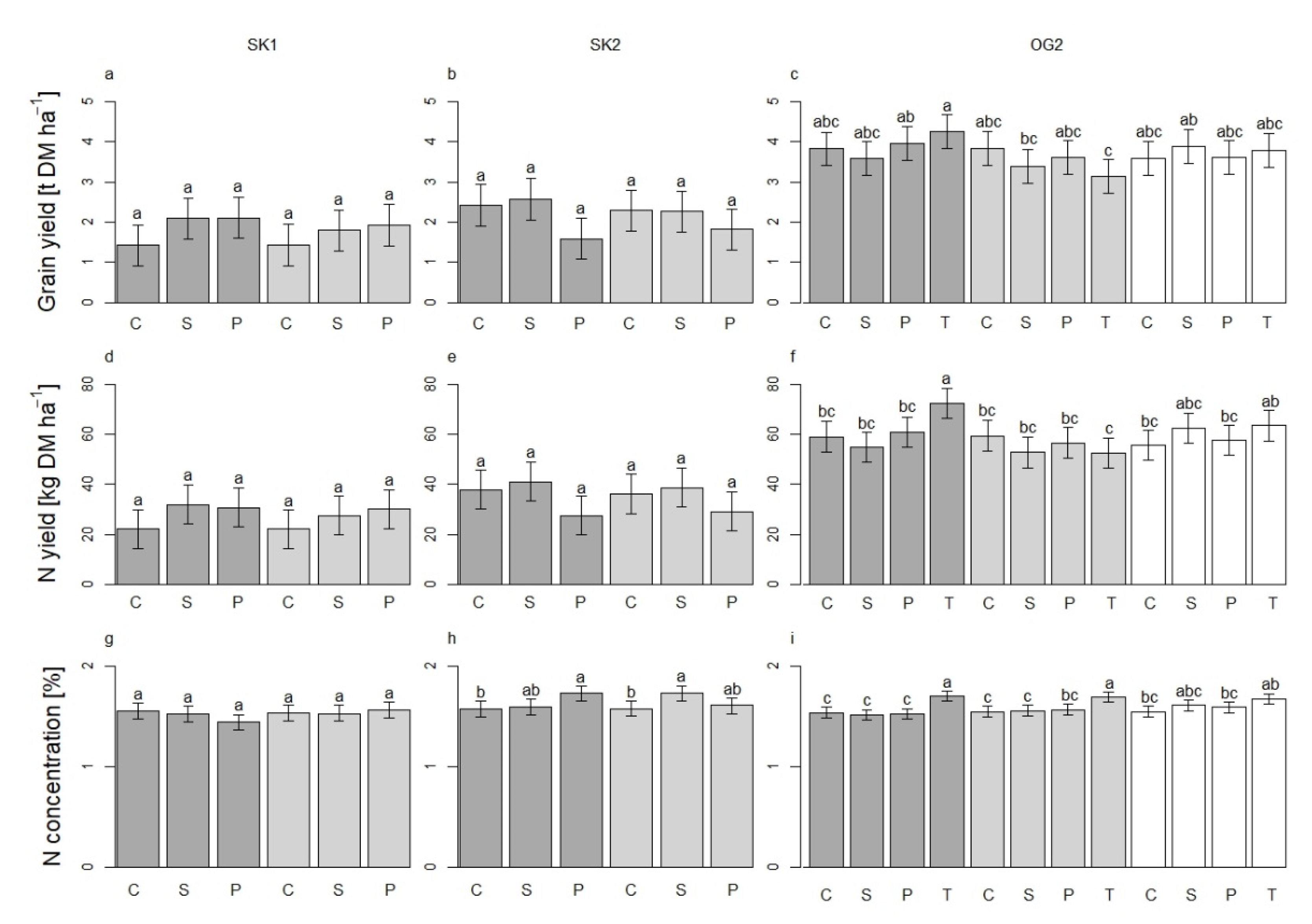
3.3. Delivery of Services and Disservices by Service Crops to the System

Effects of Service Crops on Winter Wheat Grain Yield and Nitrogen Content in Kernels

The effect of SCs on winter wheat grain yield, nitrogen (N) concentration, and N yield could not be generalised because of differences in crop performance between experiments (Figure 6). With perennial SCs, grain yield was increased compared to no SCs by an average of 0.5 t ha⁻¹ in experiment SK1 (p = 0.05), while it was reduced in experiment SK2 compared to frost-sensitive annual and no SCs (p = 0.012 and 0.02, respectively. Figure 6b). System strategy Early Intra yielded more (3.9 t ha⁻¹) than Late Inter (3.5 t ha⁻¹) in experiment OG2 (p < 0.001).

Nitrogen concentration in winter wheat kernels was higher with frost-sensitive annual SCs in system strategy Late Inter and with perennial SCs in system strategy Early Intra than with no SC in experiment SK2 (Figure 6h, p = 0.04 and 0.03, respectively). In experiment OG2, N concentration was higher with frost-tolerant annual SCs than with other SCs and no SCs (p < 0.001, for all comparisons. Figure 6i). In experiment SK1, there was no difference between treatments. Nitrogen yields were largely determined by grain yield, and these two variables thus followed the same pattern (Figure 6d–f). However, with frost-tolerant annual SCs, the effect of a higher N concentration clearly improved crop performance with regard to N yield. This was seen as a relatively larger difference in N yield compared to grain yield in treatments with frost-tolerant SCs compared to other treatments.

Intercropping with SCs affected the winter wheat stand and its yield components. Winter wheat had fewer heads m⁻² in treatments with perennial SCs than with frost-sensitive annual and no SCs in SK1 and SK2 (Table S2.4, p < 0.001 and p = 0.018, respectively). However, in experiment SK1, this was compensated for by more kernels head⁻¹ with perennial SCs than with frost-sensitive annual and no SCs (Table S2.4, p = 0.014 and 0.0026, respectively). No difference in winter wheat plant numbers was observed when established in frost-sensitive annual, perennial, or no SCs. By contrast, when established in frost-tolerant SCs, the number of winter wheat plants was reduced compared to perennial and frost-sensitive annual SCs (Table S2.4, p = 0.04 and 0.06, respectively), especially with system strategy Early Intra (p_{Mixture:System} = 0.03). Despite fewer plants established with frost-sensitive annual SCs, the grain yields were highest with winter annual SCs and system strategy Early Intra (Figure 6c). During the growing season, the winter wheat crop compensated for the smaller number of plants by producing more heads per plant than in all other treatments (Table S2.4, p = 0.03, 0.014, and 0.011 for frost-sensitive annual, perennial, and no SCs, respectively), and significantly higher thousand kernel weight than in treatments with frost-sensitive annual SCs (Table S2.4 and Table S3.2, p = 0.009).

3.4. Oat Yields

Intercropping with the most productive SCs, both frost-sensitive annual and perennial SCs in SK1 and frost-tolerant annual SCs at OG1 and OG2, led to reductions in oat yields (Figure 7). In experiment SK1, frost-sensitive annual SCs reduced oat yields by 0.5 ton ha⁻¹, 11%, compared to no SC (p = 0.003). In the OG experiments, frost-tolerant annual SCs in system strategy Early Intra reduced oat yields by 0.3–0.4 t ha⁻¹ compared to all other treatments (Figure 7). No effects of SCs on the number of plants or heads were observed.

In experiment SK1 system strategy Early Intra, oats yielded 8% less than Late Inter (p = 0.002). In addition, head numbers tended to be fewer in system strategy Early Intra than in Late Inter (Table S2.5, p = 0.09). The number of oat plants was not significantly affected by system strategy in any experiment.

Intercropping with SCs did not affect heads plant⁻¹ or kernels head⁻¹ in oats. Thousand kernel weight had a tendency to be higher in treatments with system strategy Late Inter than with Early Intra (p = 0.06) and was significantly lower in 2018 than in 2017 (p < 0.001, Table S2.5).

3.5. Weed Biomass

In winter wheat in experiment SK1, weed biomass was lower with perennial SCs than with frost-sensitive annual and no SCs (p = 0.005 and 0.04, respectively). Weed biomass was especially low with perennial SCs in system strategy Late Inter (Figure 8). In experiment OG2, frost-tolerant annual SCs reduced weed biomass by 55% compared to frost-sensitive annual SCs (p = 0.03) over both system strategies. Moreover, it was clear that the lower weed biomass with perennial SCs, compared to frost-sensitive annual and no SCs, was due to the reduction in weed biomass in the winter wheat row (0.001 g m⁻², vs. 0.14 and 0.71 g m⁻² for frost-sensitive annuals and no SCs, respectively, p = 0.001). Furthermore, in experiment SK1, weed biomass in winter wheat rows was lower with system strategy Early Intra than Late Inter (p = 0.014).

In oats, frost-tolerant annual SCs reduced weed biomass by 80% compared to perennial SCs (p = 0.03), both in experiments OG1 and OG2 (Figure 8). However, due to the large variation in weed biomass between plots, no significant differences between specific treatments were observed. Moreover, weed biomass in inter-row centres was lower with system strategy Early Intra (0.037 g m⁻²) than Late Inter (0.14 g m⁻², p = 0.06).

3.6. Soil Mineral Nitrogen

No general effects of SC or system strategy on profile SMN (0–60 and 0–90 cm) in autumn were observed, but there was an interaction between SC mixture and system strategy (Table S2.8). Frost-sensitive annual SCs resulted in the highest amount of SMN when sown early, but among the late-sown treatments, it had the lowest SMN (p = 0.017, Figure 9). The same pattern could also be observed in the topsoil (0–30 cm) but not in the other soil layers (Table S2.8). Frost-tolerant annual SCs did not affect SMN significantly compared to other SCs and the control, and SMN was at an intermediate level compared to them, both with system strategy Early Intra and Late Inter (data not shown).

In spring 2019, in experiment SK2, SMN was slightly higher with system strategy Early Intra (27 kg N ha⁻¹) than with Late Inter (23 kg N ha⁻¹, p = 0.017). This was mainly due to the difference in the 0–30 cm soil layer (19 kg N ha⁻¹ with system strategy Early Intra and 15 kg N ha⁻¹ with Late Inter). At 60–90 cm depth over both experiments, treatments with perennial SCs had lower SMN than those with no SC (p = 0.03; 4.8 kg N ha⁻¹ and 6.5 kg N ha⁻¹, respectively). There was much more SMN in experiment OG2, 49 kg ha⁻¹, than in experiment SK2, 25 kg ha⁻¹, but no differences between treatments in experiment OG2 (Table S2.9).

4. Discussion

The frost-tolerant annual service crop (SC), the mixture with Vicia villosa and Trifolium incarnatum, sown early, showed the best overall service provision. This treatment resulted in the highest grain and nitrogen (N) yields, N concentrations (Figure 6), and among the lowest weed biomass (Figure 8). The drawback was the vigorous early growth of this SC, which reduced the yield of oats (Figure 7).

In the following discussion, we will address the different aspects of the system and how service delivery can be enhanced and disservices avoided by crop management in terms of species choice and system strategy.

4.1. Nitrogen Provision for Yield and Grain Nitrogen Content in Winter Wheat

Only treatments with early sown frost-tolerant annual SCs showed a significant increase in both grain yield and N concentration for winter wheat (Figure 6). In experiment SK1, all SC treatments increased grain yield by 0.5 t ha⁻¹ compared to those with no SCs, despite varying SC growth, maybe because the drought caused generally low yields this year, lowering crop nutrient demand. Moreover, at SK1, SCs did not affect grain N concentration, which could be due to low access to soil mineral nitrogen (SMN) during this dry summer.

The timing of N availability from SC residues is an important aspect of this system. Winter wheat does not take up much N until the beginning of stem-elongation in late spring, so N released following early decay of senescing or frost-killed SCs is at risk of being lost. In our experiment, early sown frost-sensitive annuals left behind more SMN in autumn than all other treatments, probably due to the combination of high biomass production in oats and decomposition of SC material after oat harvest. Little effect of T. resupinatum, one of our frost-sensitive annual SCs, on the subsequent crop was observed in another study, which was attributed to winter wilting of the legume and subsequent N leaching [30]. However, when managed appropriately according to the conditions in the field, even leguminous SCs can reduce N leaching [31]. In our experiments, SMN was not increased by SC mixtures, which remained vigorous throughout autumn. Letting SCs remain throughout the winter instead of ploughing them down in autumn is a method for keeping SMN low [32]. Finding a suitable termination time must, however, take into consideration other factors affecting nutrient availability, such as the chemical composition of the SCs [33,34,35] and weather conditions [36], as well as the practicality for farmers. Under expected wet and mild conditions, termination should occur relatively late since the risk of leaching and gaseous emissions increases with increased precipitation [33,37,38], while when precipitation is low, N provision to the subsequent crop is improved by early termination [36]. Furthermore, traffic with heavy machines on wet soils increases the risk of soil compaction [39]. Since weather cannot be reliably predicted over longer periods and farmers must adapt their management to soil conditions, knowledge of typical local weather patterns must be used to decide termination time. Furthermore, in our experiments, the reduced tillage probably affected N availability as well. Soils under reduced and no tillage tend to warm up slower compared to ploughed [40], which can delay or slow down decomposition and mineralization. The low soil disturbance desired in these systems hence risks affecting soil temperature and associated N availability in a way that is negative to crop growth and development.

4.2. Weed Suppression

The most consistent weed suppression was observed with frost-tolerant annual SCs, in which the dominating species V. villosa (Figure 4c,d) probably made the main contribution. With this mixture, weeds were suppressed in both oats and winter wheat, with both early and late sowing (Figure 8c,d). A similar effect of V. villosa has been observed by others and was correlated to fast establishment, high biomass productivity, and large amounts of SC residues [41]. Perennial SCs, which provided relatively suitable soil cover in autumn, reduced weed biomass in winter wheat but did not reduce weed biomass in oats (Figure 8), in which they generally had small biomass production (Figure 4a–d).

Scaling down the weed biomass assessment to subsections of the plots showed that in oats, higher row hoeing intensity decreased weed biomass in inter-row centres. This was expected and confirmed other findings [42]. However, close to the cash crop rows, row hoeing intensity did not matter, which could be because the hoe did not reach all the way to the crop row. It was also observed that weeds were not always cut off by the hoe but pushed to the side. Plants uprooted by mechanical control have been shown to have about a 50% survival rate; moist soil conditions increase the chance [43]. The main effect of mechanical weed control is that it reduces weed biomass and increases crop yield [44], but sometimes it can also affect the crop negatively. In SK1, we could observe damages on oats after the second-row hoeing, which was reflected in the yields. Hence, some care needs to be taken with the mechanical weeding, although going in close proximity to the crop row is important for effective weed control. In addition, in winter wheat in SK2 and OG2, better weed control would have been needed.

The smaller weed biomass in winter wheat with perennial SCs was only observed in the crop rows. This is of particular interest since it is more difficult to manage weeds within than between cash crop rows, where row hoeing can efficiently remove weeds [44,45,46]. However, the perennial SCs were difficult to terminate in the second year and hence continued to grow in or close to the winter wheat row (data not shown), contributing to weed suppression in winter wheat, which was not seen for the other treatments in this experiment. This points to the importance of continuous competition for weed suppression in this system. However, having a vigorous SC providing this competition involves a high risk of negatively affecting the crop, as was also observed in our study.

The highest weed biomass was observed in treatments with frost-sensitive annual SCs. This was probably due to a combination of increased SMN and the lack of competition after oat harvest with this SC. The weed community composition is formed by agronomic management, and many plants that have become agricultural weeds have a high affiliation to N [47,48]. Our results show that early termination of a highly productive SC may give weeds an advantage over winter wheat when mechanical and chemical weed control is low.

4.3. Oats–Service Crop Interaction

In the majority of the treatments, oat yields were not reduced by the SCs (Figure 7). This goes in line with other studies on relay intercropping with legumes and other crops [13,31,49,50]. In these studies, the SCs are, however, under-sown at a later stage in the cash crop’s development, which gives the cash crop a greater advantage. In our experiments, late sowing was the safest way to establish the SCs to prevent competition. It has been shown that if the SC biomass is 20% or more of the cash crop biomass, cash crop grain protein content and, to a lesser extent, cash crop yield can be reduced [51]. However, high SC biomass alone does not explain the yield reduction. Frost-sensitive annual SCs in system strategy Early Intra in experiment OG1 did not decrease oat yields, despite reaching the same biomass as the frost-tolerant annual SCs. Furthermore, in experiment SK1, less productive SCs reduced oat yields compared to the control. The negative effect of the frost-tolerant annuals could be because they grew through the oat canopy and competed for light during grain filling, while the frost-sensitive annuals did not grow out of the oat canopy in OG. In experiment SK1, the reduction in oat yield even with less productive SCs could partly be due to a narrower row spacing in experiment SK1 (25 cm compared to 33 cm in the OG experiments and 32 cm in experiment SK2), increasing the competitive impact of SCs on oats in SK1.

4.4. Service Crop Performance and Species Choice

Early sowing of SCs resulted in larger biomass production than with late sowing for all SC mixtures (Figure 4a–d). This was expected since they had a longer growth period, and the oat crop did not have much of an advantage over the SC in acquiring resources in terms of light, water, and nutrients, in contrast with late-sown SCs. The difference was, however, larger for the annual than for the perennial SCs, for which sowing time was of less importance. The relatively vigorous growth of late-sown SCs in experiment SK1 indicates that water was the most limiting factor for SC growth in our experiments. This experiment received a more even distribution of precipitation in spring and summer in the establishment year compared to all other experiments (Figure 1). The performance of oats was similar in the two experiments (Figure 7). Furthermore, a trade-off between biomass production during summer and soil cover in autumn was observed for most SC mixtures. The exception was early sown frost-tolerant annual SCs, which provided both.

The analysis showed that high biomass production of SC was essential to increase grain and N yield of winter wheat and reduce weed biomass, although stronger and more consistent effects are desirable. Earlier studies have shown that an SC biomass around 2 t ha⁻¹ significantly increases the grain and N yield of the subsequent crop and reduces weed biomass [13,52]. However, because of the low soil cover by the SCs that provided the most biomass during summer, combined with the reduction in yield of oats (already at 1 t SC biomass ha⁻¹), a high SC biomass production during summer should probably not be the target in this system. Increasing the soil cover in autumn is hence a better target for service delivery in these types of systems, especially for weed control [16]. Under similar climatic conditions to ours, a 6-fold increase in biomass of under-sown SCs from cash crop harvest to November was observed [13]. However, a 6-fold increase in biomass of late-sown SCs in OG1 and of all SCs, except the frost-tolerant annual, in 2018 with both system strategies and in both experiments would still result in low final biomass before winter. Species choice and sowing time need to be adapted to local conditions to ensure sufficient soil cover in autumn. Increasing the SC sowing density is a way of increasing biomass production and soil cover. More studies are needed to gain a better understanding of how SC biomass production can be managed to provide the desired services without suppressing the cash crop by choice of species and cultivars, as well as by adjusting the time and density of sowing under different pedo-climatic conditions.

In our experiments, most SCs gained 60–85% of their N from the atmosphere, similar to other observations [8]. The exception was M. lupulina. Forming symbioses with natural rhizobial communities has shown to be more difficult for Medicago species compared to Trifolium species, probably because of a lower presence of bacterial strains that form a symbiosis with Medicago species in agricultural soils [53]. Generally, perennial SCs had slightly lower %Ndfa than annual SCs, except in SK1. The %Ndfa is often correlated with biomass production [54]. In our study, perennial SCs in experiment SK1 showed both higher biomass and %Ndfa than perennials in all other experiments, which supports the positive correlation between legume biomass and %Ndfa. Water availability is another factor influencing the ability of N₂ fixation [55,56], and the greater fixation found in SK1 could also be explained by greater water availability than in the other experiments. The perennials grew slower than the annuals at the beginning of the season, but at SK1, with an excess of water, perennial and frost-sensitive annuals showed similar %Ndfa. In 2018, %Ndfa was greatly reduced in OG2, which could be due to the poor growth and lack of water; this was, however, not expected to have differed much compared to the conditions in SK2. The higher soil organic matter content at OG2 than at SK2, indicating a greater potential for N mineralization from the OG2 soil, combined with lower phosphorus (P) content, could have disfavoured N₂ fixation at OG2 compared to SK2 since the high availability of N and low availability of P constrain biological N₂ fixation [57]. Hence, many factors influence the ability of legumes to provide the cropping system with nitrogen. Although legume biomass production is the main factor influencing N input [56,58,59], legume species choice and crop management need to be carefully chosen if the cropping system should rely less on external inputs.

The severe drought in 2018 provided insights into the tolerance of the different species to the combination of water and heat stress. The only SC that showed significant growth in 2018 was V. villosa. Its fast establishment and growth were probably beneficial in this dry year. Vicia villosa also has hairs covering the leaves, which is known to reduce transpiration [60,61]. These extreme weather events are expected to become more common in the future [62]; hence, drought tolerance of SCs will be another trait to consider. However, access to irrigation is probably necessary to ensure the high and stable growth of SCs under variable weather and soil conditions.

4.5. Developing (Relay) Intercropping Systems with Forage Legumes

In this study, SC species mixtures were grouped according to longevity and frost sensitivity to distinguish between different growth dynamics. Different establishment strategies of under-sowing in a spring cereal were tested under northern European growth conditions. Early sown frost-tolerant annuals showed to be the most favourable for improving yields and providing weed control due to high productivity in summer, recovery after oat harvest, and winter hardiness. Service crops showing other growth dynamics failed in service provision, at least partly, or even caused disservices. When the SCs established slowly, they generally did not reduce weed biomass and had too little biomass in late summer for sufficient growth in autumn, and did not increase the yield of the subsequent winter wheat. When the SCs grew fast in the beginning but did not recover after oat harvest, they increased SMN in autumn, which could be leached out of the field or fertilize weeds. Species combinations that mix groups of species might provide similar positive effects as the frost-tolerant annuals if the above-mentioned combination is achieved and could even improve this dynamic. Mixing species allows the complementarity in species traits to be exploited [18,63] or to guarantee that at least one species will do well [18,64]. Having identified promising trait combinations for service delivery in our system, future studies should explore how more complex mixtures can be composed in this or similar systems.

Biomass production and hence the potential service provision of SCs varied between years. This has also been observed in other studies (e.g., [41,65]) and calls for a better understanding of how variations in environmental conditions affect different SC species and how cropping system design, including SC choice and crop management, might enhance SC productivity and delivery of different services. Mixtures with both diversity and redundancy in traits have been shown to better cope with stressful environments [64]. However, the more species that are included, the harder it will be to evaluate the effect of the specific species on the overall performance and hence understand how the mixture will perform in other environments.

Many services could be desired from an agricultural system, and it is difficult to avoid trade-offs [66,67]. In our system, the clearest trade-off risk occurs from the biomass produced for weed suppression and nutrient accumulation and the competition with oats. However, if other services were to be taken into account, additional trade-offs might become evident.

Finally, we have identified some technical aspects of the system in need of improvement to make the system more robust and farmer friendly. These are to ensure a more even establishment of both cash crops and SCs in this intercropped and direct-seeded system and better removal of both weeds and SCs.

5. Conclusions

There are many aspects to consider when designing and managing SCs in intercropping systems. The positive effects on grain and nitrogen yield and weed suppression show that there is potential in this system, but the varying SC growth and following effects on winter wheat yields and weed control indicate that the system needs further optimization. This optimization should aim at ensuring suitable SC establishment before oat harvest so that the SC can fill the empty space and, by doing so, suppress weeds and retain nutrients to become available the following spring. The best performing SC mixture in our study was with frost-tolerant annuals in system strategy Early Intra. This treatment combination resulted in a large SC biomass in oats, which recovered after the harvest of oats and stayed alive during winter. Hence, high productivity of the SC seems to be key to producing the desired services but also increases the risk of potential disservices such as competition and nitrogen leaching. Other species, or combinations of species, probably have the potential to do the same if the aforementioned growth dynamics are achieved.

References

1. Kremen, C. Managing Ecosystem Services: What Do We Need to Know about Their Ecology? Ecol. Lett. 2005, 8, 468–479. [Google Scholar] [CrossRef] [PubMed]
2. Nivelle, E.; Verzeaux, J.; Habbib, H.; Kuzyakov, Y.; Decocq, G.; Roger, D.; Lacoux, J.; Duclercq, J.; Spicher, F.; Nava-Saucedo, J.E.; et al. Functional Response of Soil Microbial Communities to Tillage, Cover Crops and Nitrogen Fertilization. Appl. Soil Ecol. 2016, 108, 147–155. [Google Scholar] [CrossRef]
3. Verret, V.; Gardarin, A.; Pelzer, E.; Médiène, S.; Makowski, D.; Valantin-Morison, M. Can Legume Companion Plants Control Weeds without Decreasing Crop Yield? A Meta-Analysis. F. Crop. Res. 2017, 204, 158–168. [Google Scholar] [CrossRef]
4. Blanco-Canqui, H.; Holman, J.D.; Schlegel, A.J.; Tatarko, J.; Shaver, T.M. Replacing Fallow with Cover Crops in a Semiarid Soil: Effects on Soil Properties. Soil Sci. Soc. Am. J. 2013, 77, 1026–1034. [Google Scholar] [CrossRef]
5. Askegaard, M.; Eriksen, J. Residual Effect and Leaching of N and K in Cropping Systems with Clover and Ryegrass Catch Crops on a Coarse Sand. Agric. Ecosyst. Environ. 2008, 123, 99–108. [Google Scholar] [CrossRef]
6. Liu, J.; Bergkvist, G.; Ulén, B. Biomass Production and Phosphorus Retention by Catch Crops on Clayey Soils in Southern and Central Sweden. F. Crop. Res. 2015, 171, 130–137. [Google Scholar] [CrossRef]
7. Poeplau, C.; Don, A. Carbon Sequestration in Agricultural Soils via Cultivation of Cover Crops—A Meta-Analysis. Agric. Ecosyst. Environ. 2015, 200, 33–41. [Google Scholar] [CrossRef]
8. Büchi, L.; Gebhard, C.A.; Liebisch, F.; Sinaj, S.; Ramseier, H.; Charles, R. Accumulation of Biologically Fixed Nitrogen by Legumes Cultivated as Cover Crops in Switzerland. Plant Soil 2015, 393, 163–175. [Google Scholar] [CrossRef]
9. Wendling, M.; Büchi, L.; Amossé, C.; Sinaj, S.; Walter, A.; Charles, R. Influence of Root and Leaf Traits on the Uptake of Nutrients in Cover Crops. Plant Soil 2016, 409, 419–434. [Google Scholar] [CrossRef]
10. Scavo, A.; Restuccia, A.; Abbate, C.; Lombardo, S.; Fontanazza, S.; Pandino, G.; Anastasi, U.; Mauromicale, G. Trifolium Subterraneum Cover Cropping Enhances Soil Fertility and Weed Seedbank Dynamics in a Mediterranean Apricot Orchard. Agron. Sustain. Dev. 2021, 41, 70. [Google Scholar] [CrossRef]
11. Verret, V.; Pelzer, E.; Bedoussac, L.; Jeuffroy, M.H. Tracking on-Farm Innovative Practices to Support Crop Mixture Design: The Case of Annual Mixtures Including a Legume Crop. Eur. J. Agron. 2020, 115, 126018. [Google Scholar] [CrossRef]
12. Finney, D.M.; White, C.M.; Kaye, J.P. Biomass Production and Carbon/Nitrogen Ratio Influence Ecosystem Services from Cover Crop Mixtures. Agron. J. 2016, 108, 39–52. [Google Scholar] [CrossRef]
13. Bergkvist, G.; Stenberg, M.; Wetterlind, J.; Båth, B.; Elfstrand, S. Clover Cover Crops Under-Sown in Winter Wheat Increase Yield of Subsequent Spring Barley-Effect of N Dose and Companion Grass. F. Crop. Res. 2011, 120, 292–298. [Google Scholar] [CrossRef]
14. Zhao, J.; De Notaris, C.; Olesen, J.E. Autumn-Based Vegetation Indices for Estimating Nitrate Leaching during Autumn and Winter in Arable Cropping Systems. Agric. Ecosyst. Environ. 2020, 290, 106786. [Google Scholar] [CrossRef]
15. Aronsson, H.; Hansen, E.M.; Thomsen, I.K.; Liu, J.; Øgaard, A.F.; Känkänen, H.; Ulén, B. The Ability of Cover Crops to Reduce Nitrogen and Phosphorus Losses from Arable Land in Southern Scandinavia and Finland. J. Soil Water Conserv. 2016, 71, 41–55. [Google Scholar] [CrossRef]
16. Reimer, M.; Ringselle, B.; Bergkvist, G.; Westaway, S.; Wittwer, R.; Baresel, J.P.; Van Der Heijden, M.G.A.; Mangerud, K.; Finckh, M.R.; Brandsæter, L.O. Interactive Effects of Subsidiary Crops and Weed Pressure in the Transition Period to Non-Inversion Tillage, a Case Study of Six Sites across Northern and Central Europe. Agronomy 2019, 9, 495. [Google Scholar] [CrossRef]
17. De Baets, S.; Poesen, J.; Meersmans, J.; Serlet, L. Cover Crops and Their Erosion-Reducing Effects during Concentrated Flow Erosion. Catena 2011, 85, 237–244. [Google Scholar] [CrossRef]
18. Justes, E.; Bedoussac, L.; Dordas, C.; Frak, E.; Louarn, G.; Boudsocq, S.; Journet, E.P.; Lithourgidis, A.; Pankou, C.; Zhang, C.; et al. The 4 C Approach as a Way to Understand Species Interactions Determining Productivity. Front. Agric. Sci. Eng. 2021, 8, 387–399. [Google Scholar] [CrossRef]
19. Blackshaw, R.E.; Moyer, J.R.; Doram, R.C.; Boswall, A.L.; Smith, E.G. Suitability of Undersown Sweetclover as a Fallow Replacement in Semiarid Cropping Systems. Agron. J. 2001, 93, 863–868. [Google Scholar] [CrossRef]
20. Walter, H.; Lieth, H.H.F. Klimadiagramm-Weltatlas; Jena, G., Ed.; Fischer Verlag: Jena, Germany, 1967. [Google Scholar]
21. Werner, R.A.; Bruch, B.A.; Brand, W.A. ConFlo III—An Interface for High Precision d 13 C and d 15 N Analysis with an Extended Dynamic Range. Rapid Commun. Mass Spectrom. 1999, 13, 1237–1241. [Google Scholar] [CrossRef]
22. Shearer, G.; Kohl, D.H. N2-Fixation in Field Settings: Estimations Based on Natural 15N Abundance. Aust. J. Plant Physiol. 1986, 13, 699–756. [Google Scholar] [CrossRef]
23. Roscher, C.; Thein, S.; Weigelt, A.; Temperton, V.M.; Buchmann, N.; Schulze, E.; Weigelt, A. N2 Fixation and Performance of 12 Legume Species in a 6-Year Grassland Biodiversity Experiment. Plant Soil 2011, 341, 333–348. [Google Scholar] [CrossRef]
24. Eriksen, J.; Høgh-Jensen, H. Variations in the Natural Abundance of 15 N in Ryegrass/White Clover Shoot Material as Influenced by Cattle Grazing. Plant Soil 1998, 205, 67–76. [Google Scholar] [CrossRef]
25. R Core Team. R: A Language and Environment for Statistical Computing. R Foundation for Statistical Computing, Vienna, Austria. Available online: https://www.r-project.org/ (accessed on 4 January 2021).
26. Bates, D.; Maechler, M.; Bolker, B.; Walker, S. Package ‘Lme4’ Linear Mixed-Effects Models Using “Eigen” and S4. Available online: https://cran.r-project.org/web/packages/lme4/index.html (accessed on 2 August 2022).
27. Fox, J.; Weisberg, S.; Price, B.; Adler, D.; Bates, D.; Baud-Bovy, G.; Bolker, B.; Ellison, S.; Firth, D.; Friendly, M.; et al. Car: Companion to Applied Regression. Available online: https://cran.r-project.org/web/packages/car/index.html (accessed on 2 August 2022).
28. Russell, A.; Lenth, V.; Buerkner, P.; Herve, M.; Love, J.; Singmann, H.; Lenth, M.R. V Package ‘ Emmeans ’ R Topics Documented. 2022. Available online: https://cran.r-project.org/web/packages/emmeans/ (accessed on 2 August 2022).
29. Wickham, H. Elegant Graphics for Data Analysis; Springer: New York, NY, USA, 2016; ISBN 978-3-319-24277-4. [Google Scholar]
30. Askegaard, M.; Eriksen, J. Growth of Legume and Nonlegume Catch Crops and Residual-N Effects in Spring Barley on Coarse Sand. J. Plant Nutr. Soil Sci. 2007, 170, 773–780. [Google Scholar] [CrossRef]
31. Noland, R.L.; Wells, M.S.; Sheaffer, C.C.; Baker, J.M.; Martinson, K.L.; Coulter, J.A. Establishment and Function of Cover Crops Interseeded into Corn. Crop Sci. 2018, 58, 863–873. [Google Scholar] [CrossRef]
32. Arlauskienė, A.; Gecaitė, V.; Toleikienė, M.; Šarūnaitė, L.; Kadžiulienė, Ž. Soil Nitrate Nitrogen Content and Grain Yields of Organically Grown Cereals as Affected by a Strip Tillage and Forage Legume Intercropping. Plants 2021, 10, 1453. [Google Scholar] [CrossRef] [PubMed]
33. Thorup-Kristensen, K. The Effect of Nitrogen Catch Crops on The Nitrogen Nutrition of A Succeeding Crop I. Effects Through Mineralization and Pre-Emptive Competition. Acta Agric. Scand. Sect. B Soil Plant Sci. 1993, 43, 74–81. [Google Scholar] [CrossRef]
34. Wivstad, M. Nitrogen Mineralization and Crop Uptake of N from Decomposing 15N Labelled Red Clover and Yellow Sweetclover Plant Fractions of Different Age. Plant Soil 1999, 208, 21–31. [Google Scholar] [CrossRef]
35. Magid, J.; Henriksen, O.; Thorup-kristensen, K.; Mueller, T. Disproportionately High N-Mineralisation Rates from Green Manures at Low Temperatures—Implications for Modeling and Management in Cool Temperate Agro-Ecosystems. Plant Soil 2001, 228, 73–82. [Google Scholar] [CrossRef]
36. Thorup-Kristensen, K.; Dresbøll, D.B. Incorporation Time of Nitrogen Catch Crops Influences the N Effect for the Succeeding Crop. Soil Use Manag. 2010, 26, 27–35. [Google Scholar] [CrossRef]
37. Tosti, G.; Farneselli, M.; Benincasa, P.; Guiducci, M. Nitrogen Fertilization Strategies for Organic Wheat Production: Crop Yield and Nitrate Leaching. Agron. J. 2016, 108, 770–781. [Google Scholar] [CrossRef]
38. Rochette, P.; Liang, C.; Pelster, D.; Bergeron, O.; Lemke, R.; Kroebel, R.; MacDonald, D.; Yan, W.; Flemming, C. Soil Nitrous Oxide Emissions from Agricultural Soils in Canada: Exploring Relationships with Soil, Crop and Climatic Variables. Agric. Ecosyst. Environ. 2018, 254, 69–81. [Google Scholar] [CrossRef]
39. Hamza, M.A.; Anderson, W.K. Soil Compaction in Cropping Systems: A Review of the Nature, Causes and Possible Solutions. Soil Tillage Res. 2005, 82, 121–145. [Google Scholar] [CrossRef]
40. Shen, Y.; McLaughlin, N.; Zhang, X.; Xu, M.; Liang, A. Effect of Tillage and Crop Residue on Soil Temperature Following Planting for a Black Soil in Northeast China. Sci. Rep. 2018, 8, 4500. [Google Scholar] [CrossRef]
41. Dorn, B.; Jossi, W.; van der Heijden, M.G.A. Weed Suppression by Cover Crops: Comparative on-Farm Experiments under Integrated and Organic Conservation Tillage. Weed Res. 2015, 55, 586–597. [Google Scholar] [CrossRef]
42. Cirujeda, A.; Melander, B.; Rasmussen, K.; Rasmussen, I.A. Relationship between Speed, Soil Movement into the Cereal Row and Intra-Row Weed Control Efficacy by Weed Harrowing. Weed Res. 2003, 43, 285–296. [Google Scholar] [CrossRef]
43. Kurstjens, D.A.G.; Kropff, M.J. The Impact of Uprooting and Soil-Covering on the Effectiveness of Weed Harrowing. Weed Res. 2001, 41, 211–288. [Google Scholar] [CrossRef]
44. Jacobsen, S.E.; Christiansen, J.L.; Rasmussen, J. Weed Harrowing and Inter-Row Hoeing in Organic Grown Quinoa (Chenopodium Quinoa Willd.). Outlook Agric. 2010, 39, 223–227. [Google Scholar] [CrossRef]
45. Kolb, L.N.; Gallandt, E.R.; Molloy, T. Improving Weed Management in Organic Spring Barley: Physical Weed Control vs. Interspecific Competition. Weed Res. 2010, 50, 597–605. [Google Scholar] [CrossRef]
46. Melander, B.; Jabran, K.; De Notaris, C.; Znova, L.; Green, O.; Olesen, J.E. Inter-Row Hoeing for Weed Control in Organic Spring Cereals—Influence of Inter-Row Spacing and Nitrogen Rate. Eur. J. Agron. 2018, 101, 49–56. [Google Scholar] [CrossRef]
47. Fried, G.; Chauvel, B.; Reboud, X. A Functional Analysis of Large-Scale Temporal Shifts from 1970 to 2000 in Weed Assemblages of Sunflower Crops in France. J. Veg. Sci. 2009, 20, 49–58. [Google Scholar] [CrossRef]
48. Storkey, J.; Moss, S.R.; Cussans, J.W. Using Assembly Theory to Explain Changes in a Weed Flora in Response to Agricultural Intensification. Weed Sci. 2010, 58, 39–46. [Google Scholar] [CrossRef]
49. Amosse, C.; Mary, B.; David, C. Contribution of Relay Intercropping with Legume Cover Crops on Nitrogen Dynamics in Organic Grain Systems. Nutr. Cycl. Agroecosystems 2014, 98, 1–14. [Google Scholar] [CrossRef]
50. Vrignon-Brenas, S.; Celette, F.; Amossé, C.; David, C. Effect of Spring Fertilization on Ecosystem Services of Organic Wheat and Clover Relay Intercrops. Eur. J. Agron. 2016, 73, 73–82. [Google Scholar] [CrossRef]
51. Amossé, C.; Jeuffroy, M.H.; David, C. Relay Intercropping of Legume Cover Crops in Organic Winter Wheat: Effects on Performance and Resource Availability. F. Crop. Res. 2013, 145, 78–87. [Google Scholar] [CrossRef]
52. Vrignon-Brenas, S.; Celette, F.; Piquet-Pissaloux, A.; David, C. Biotic and Abiotic Factors Impacting Establishment and Growth of Relay Intercropped Forage Legumes. Eur. J. Agron. 2016, 81, 169–177. [Google Scholar] [CrossRef]
53. Roberts, R.; Jackson, R.W.; Mauchline, T.H.; Hirsch, P.R.; Shaw, L.J.; Döring, T.F.; Jones, H.E. Is There Sufficient Ensifer and Rhizobium Species Diversity in UK Farmland Soils to Support Red Clover (Trifolium pratense), White Clover (T. repens), Lucerne (Medicago sativa) and Black Medic (M. lupulina)? Appl. Soil Ecol. 2017, 120, 35–43. [Google Scholar] [CrossRef]
54. Romanyà, J.; Casals, P. Biological Nitrogen Fixation Response to Soil Fertility Is Species-Dependent in Annual Legumes. J. Soil Sci. Plant Nutr. 2020, 20, 546–556. [Google Scholar] [CrossRef]
55. Pandey, A.; Li, F.; Askegaard, M.; Olesen, J.E. Biological Nitrogen Fi Xation in Three Long-Term Organic and Conventional Arable Crop Rotation Experiments in Denmark. Eur. J. Agron. 2017, 90, 87–95. [Google Scholar] [CrossRef]
56. Peoples, M.B.; Bowman, A.M.; Gault, R.R.; Herridge, D.F.; McCallum, M.H.; McCormick, K.M.; Norton, R.M.; Rochester, I.J.; Scammell, G.J.; Schwenke, G.D. Factors Regulating the Contributions of Fixed Nitrogen by Pasture and Crop Legumes to Different Farming Systems of Eastern Australia. Plant Soil 2001, 228, 29–41. [Google Scholar] [CrossRef]
57. Sanz-Saez, A.; Morales, F.; Arrese-Igor, C.; Aranjuelo, I.P. Deficiency: A Major Limiting Factor for Rhizobial Symbiosis. In Legume Nitrogen Fixation in Soils with Low Phosphorus Availability; Sulieman, S., Tran, L.-S.P., Eds.; Springer International Publishing AG: Cham, Switzerland, 2017; pp. 21–40. ISBN 978-3-319-55728-1. [Google Scholar]
58. Guiducci, M.; Tosti, G.; Falcinelli, B.; Benincasa, P. Sustainable Management of Nitrogen Nutrition in Winter Wheat through Temporary Intercropping with Legumes. Agron. Sustain. Dev. 2018, 38, 31. [Google Scholar] [CrossRef]
59. Zhang, Y.; Carswell, A.; Jiang, R.; Cardenas, L.; Chen, D.; Misselbrook, T. The Amount, but Not the Proportion, of N2 Fixation and Transfers to Neighboring Plants Varies across Grassland Soils. Soil Sci. Plant Nutr. 2020, 66, 481–488. [Google Scholar] [CrossRef]
60. Ripley, B.S.; Pammenter, N.W.; Smith, V.R. Function of Leaf Hairs Revisited: The Hair Layer on Leaves Arctotheca Populifolia Reduces Photoinhibition, but Leads to Higher Leaf Temperatures Caused by Lower Transpiration Rates. J. Plant Physiol. 1999, 155, 78–85. [Google Scholar] [CrossRef]
61. Wang, X.; Shen, C.; Meng, P.; Tan, G.; Lv, L. Analysis and Review of Trichomes in Plants. BMC Plant Biol. 2021, 21, 70. [Google Scholar] [CrossRef]
62. IPCC. Summary for Policymakers. In Climate Change 2021: The Physical Science Basis. Contribution of Working Group I to the Sixth Assessment Report of the Intergovernmental Panel on Climate Change; Cambridge University Press: Cambridge, UK, 2021; pp. 3–32. [Google Scholar]
63. Wendling, M.; Charles, R.; Herrera, J.; Amossé, C.; Jeangros, B.; Walter, A.; Büchi, L. Effect of Species Identity and Diversity on Biomass Production and Its Stability in Cover Crop Mixtures. Agric. Ecosyst. Environ. 2019, 281, 81–91. [Google Scholar] [CrossRef]
64. Ranaldo, M.; Carlesi, S.; Costanzo, A.; Bàrberi, P. Functional Diversity of Cover Crop Mixtures Enhances Biomass Yield and Weed Suppression in a Mediterranean Agroecosystem. Weed Res. 2020, 60, 96–108. [Google Scholar] [CrossRef]
65. Wayman, S.; Kissing Kucek, L.; Mirsky, S.B.; Ackroyd, V.; Cordeau, S.; Ryan, M.R. Organic and Conventional Farmers Differ in Their Perspectives on Cover Crop Use and Breeding. Renew. Agric. Food Syst. 2017, 32, 376–385. [Google Scholar] [CrossRef]
66. Schipanski, M.E.; Barbercheck, M.; Douglas, M.R.; Finney, D.M.; Haider, K.; Kaye, J.P.; Kemanian, A.R.; Mortensen, D.A.; Ryan, M.R.; Tooker, J.; et al. A Framework for Evaluating Ecosystem Services Provided by Cover Crops in Agroecosystems. Agric. Syst. 2014, 125, 12–22. [Google Scholar] [CrossRef]
67. Daryanto, S.; Fu, B.; Wang, L.; Jacinthe, P.A.; Zhao, W. Quantitative Synthesis on the Ecosystem Services of Cover Crops. Earth-Sci. Rev. 2018, 185, 357–373. [Google Scholar] [CrossRef]
Figure 1. Meteorological data from the weather station closest to the experiments in SK and OG expressed in Walter–Leith graphs [20] for the three experimental years: 2017 at the top, 2018 in the middle, and 2019 at the bottom. The blue thick solid lines represent monthly precipitation, and the red solid lines represent average monthly temperature. The blue striped areas indicate excess water, and the red dotted areas indicate periods of (likely) water deficit, i.e., periods with precipitation less than two times the average monthly temperature. The number in parentheses after the site name is the altitude at the site. The numbers at the top are mean temperature of the year (middle) and accumulated precipitation during the year (right). The numbers to the left of the y-axes are the mean temperature of the warmest (top) and coldest (bottom) month. The dark turquoise boxes at the bottom indicate months when frost temperatures are common, and the light turquoise boxes indicate when frost could occur.
Agriculture 12 01398 g001
Figure 2. Visualization of the study system. (a) Timeline of crops grown in the field and main expected service delivery. In oats, the service crop mainly builds up biomass for later service provision. (b) Visualization of the placement of service crops depending on system strategy. From the left: Early Intra (service crop sown in crop row), Late Inter (service crop sown in inter-row centres at first row hoeing), and Late Adjacent (service crops sown adjacent to crop row at first row hoeing). All pictures are of the frost-sensitive annual service crop mixtures, Trifolium resupinatum and T. squarrosum. Photos by E. Lagerquist, experiment OG1, July 2017.
Agriculture 12 01398 g002
Figure 3. (a) Sketch over a plot and where data were collected for the different measurements and crops. For the data collection in oats (black squares) in OG1, only three frames were used. In this case, one frame was used instead of two at one end of the plot and located in the centre of the sampling area. The yellow stripes represent the cereal rows to demonstrate how samples were collected in relation to these. (b) Subsections for weed biomass sampling in both oats and winter wheat. Abbreviations: ir = in crop row, cr = close to crop row, ic = inter-row centres.
Agriculture 12 01398 g003
Figure 4. Service crop biomass before oat harvest (ad) and soil cover in autumn (eh) at the four experimental sites. Abbreviations: SK and OG stands for the two experimental regions, 1 = starting 2017, 2 = starting 2018, C = no service crop, S = frost-sensitive annuals, P = perennials, T = frost-tolerant annuals. Biomass values are back-transformed from log-transformed model estimates. In biomass plots the grey scale indicates the species in the mixtures: gray = Trifolium squarrosum (S), T. pratense (P) and Vicia villosa (T), white = T. resupinatum (S), T. repens (P), and T. incarnatum (T), black = Medicago lupulina (P). Early and Late indicate system strategy. See Materials and Methods and Table 1 for detailed information. Error bars indicate the 95% confidence interval for the total biomass and soil cover, respectively. The letters indicate significant differences between treatments within each experiment.
Agriculture 12 01398 g004
Figure 5. Percent of nitrogen derived from the atmosphere [%Ndfa] before winter in the forage legumes at the four experiments. Abbreviations: SK and OG stand for the two experimental regions, 1 = starting 2017, 2 = starting 2018. Point shapes indicate mixture: frost-sensitive annuals (squares), perennials (circles), and frost-tolerant annuals (triangles). T.res = Trifolium resupinatum, T.squ = T. squarrosum, M.lup = Medicago lupulina, T.pra = T. pratense, T.rep = T. repens, V.vil = Vicia villosa, and T.inc = T. incarnatum. Error bars indicate the 95% confidence interval, and the letters indicate significant differences between treatments within each experiment.
Agriculture 12 01398 g005
Figure 6. Dry matter (DM) grain yield (ac), nitrogen yield (df), and nitrogen concentration in kernels (gi) of winter wheat in the three experiments. Abbreviations: SK and OG stands for the two experimental regions, 1 = starting 2017, 2 = starting 2018, C = no service crop, S = frost-sensitive annuals, P = perennials, T = frost-tolerant annuals. No data are presented for winter wheat in the OG1 experiment since spring wheat was grown here this year. Colour coding indicating system strategy: dark grey = Early Intra, light grey = Late Inter, white = Late Adjacent. See Materials and Methods and Table 1 for information on treatments. Error bars indicate the 95% confidence interval, and the letters indicate significant differences between treatments within each experiment.
Agriculture 12 01398 g006
Figure 7. Oat dry matter (DM) grain yield in the four experiments (ad). Abbreviations: SK and OG stands for the two experimental regions, 1 = starting 2017, 2 = starting 2018, C = no service crop, S = frost-sensitive annuals, P = perennials, T = frost-tolerant annuals. Colour coding: dark grey = Early Intra, light grey = Late Inter, white = Late Adjacent. See Materials and Methods and Table 1 for detailed information. Error bars indicate the 95% confidence interval, and the letters indicate significant differences between treatments within each experiment.
Agriculture 12 01398 g007
Figure 8. Weed biomass in oats (ad) and winter wheat (eg) before cash crop harvest. Biomass values are back-transformed from log-transformed model estimates. Abbreviations: SK and OG stands for the two experimental regions, 1 = starting 2017, 2 = starting 2018, SC = service crop, S = frost-sensitive annuals, P = perennials, T = frost-tolerant annuals. No data are presented for winter wheat in the OG1 experiment since spring wheat was grown here this year. The colour coding shows the biomass in the different subsections of the sampled areas: white = in crop row, grey = close to crop row, black = inter-row centres. The letters indicate significant differences in total biomass, error bars for the 95% CI were not included in the figure since the wide CIs made the mean values and proportions difficult to read. Confidence intervals can be found in Table S3.4. See Section 2 for detailed treatment explanations and Table 1 for treatment overview. Observe that y-axis values differ between crops, and that of SK1 in winter wheat differs from the two others.
Agriculture 12 01398 g008
Figure 9. Autumn soil mineral nitrogen (SMN) at 0–90 cm as treatment averages over all experiments. Colour coding indicates the amounts in each measured layer: 0–30, 30–60, and 60–90, going from light to dark grey. C = control (no service crop, SC), S = frost-sensitive annual SCs, P = perennial SCs. Error bars show the 95% confidence interval whole profile SMN. Significance letters show the statistical difference between treatments in each soil layer and should not be compared between layers.
Agriculture 12 01398 g009