Article

Long-Term Impact of Genomic Selection on Genetic Gain Using Different SNP Density

1
Institute of Animal Science, Chinese Academy of Agricultural Sciences, Beijing 100193, China
2
Henan International Joint Laboratory of Nutrition Regulation and Ecological Raising of Domestic Animal, College of Animal Science and Technology, Henan Agricultural University, Zhengzhou 450046, China
*
Author to whom correspondence should be addressed.
Agriculture 2022, 12(9), 1463; https://doi.org/10.3390/agriculture12091463
Submission received: 23 July 2022 / Revised: 29 August 2022 / Accepted: 9 September 2022 / Published: 14 September 2022
(This article belongs to the Section Farm Animal Production)

Abstract

:
Genomic selection (GS) has been widely used in livestock breeding. However, the long-term impact of GS on genetic gain, as well as inbreeding levels, has not been fully explored in beef cattle. In this study, we carried out simulation analysis using different approaches involving two types of SNP density (54 K and 100 K) and three levels of heritability traits (h2 = 0.1, 0.3, and 0.5) to explore the long-term effects of selection strategies on genetic gain and average kinship coefficients. Our results showed that GS can improve the genetic gain across generations, and the GBLUP strategy showed slightly better performance than the BayesA model. Higher trait heritability can generate higher genetic gain in all scenarios. Moreover, simulation results using GBLUP and BayesA strategies showed higher average kinship coefficients compared with other strategies. Our study suggested that it is important to design GS strategies by considering the SNP density and trait heritability to achieve long-term and sustainable genetic gain and to effectively control inbreeding levels.

1. Introduction

Genomic selection (GS) was proposed to select candidates by estimating the genetic estimated breeding values (GEBV) of individuals using the effects of whole genome-wide SNP markers [1]. This approach allows for the selection of individuals at an early stage, thereby increasing genetic gains, reducing breeding years, and shortening the generation intervals [2,3].
Simulation studies can help to explore different breeding programs, analyze the genetic architecture of complex traits, and evaluate the sources of variability. This approach can achieve rapid, multiple experiment repetitions at a very low cost, which is difficult to achieve using real data [4,5]. Many GS studies have been carried out based on simulated data.
A previous study indicated that Bayesian methods can increase GEBV prediction accuracy and selection on GEBV substantially increasing the rate of genetic gain in animals and plants based on a simulated genome [1]. Simulation analysis has proved that genomic information can increase the genetic gain rates and reduce the average inbreeding coefficient in dairy cattle [6]. In beef cattle, one recent study pointed out that GS, using simulated data, allowed better genetic progress for female reproduction and meat quality than PBLUP [7]. Similarly, analysis based on simulation suggested that the GS method had potential application for Chinese indigenous cattle [8]. Moreover, other studies using simulation also indicated that the GS method could improve prediction accuracy in animals and plants [9,10].
GS has been widely applied in many livestock and crops due to the increasing popularity of commercialized high-density SNP chips over last decade [11,12,13,14,15]. This approach has promoted the rate of genetic progress for important economic traits in dairy cattle [16]. A previous study reported that the rate of genetic gain per year increased from ~50–100% for yield traits and from three-fold to four-fold for lowly heritable traits using GS [13].
Genetic gains achieved using relevant selection methods, including GS, can evaluate the improvement or response of selection [17]. Genetic gain can be defined by the amount of increase in performance that is obtained through selection programs [18]. Several factors, including population size, trait heritability, and statistical model, should be considered to achieve high genetic gains. The effect of these factors on genetic gain is achieved indirectly by influencing the accuracy of GEBV [19]. For example, a large population size with close relationships can improve prediction accuracy [20]. Higher prediction accuracy can be obtained by applying the GS approach for highly heritable traits, as well as lowly heritable traits [21]. Different statistical models have been proposed to support GS as a powerful approach to increase genetic gain, with different prediction accuracies [22].
GS can effectively increase the genetic gain in the short-term. However, the selection of related high GEBV individuals as parents for each generation may decrease genetic diversity, lower selection response, and cause high homozygosity for deleterious alleles [23,24]. Therefore, the analysis of genetic performance in livestock is important for long-term selection in farm animals. A previous study pointed out that the average predictive accuracy of 20 important traits using GBLUP and Bayesian approaches in beef cattle was around 0.36 [22]. However, the investigation of the long-term effect of genetic gain, along with inbreeding levels from GS, is yet to be fully explored in beef cattle.
The objectives of the present study were to (1) investigate the long-term effects of applying the GS approach in beef cattle; (2) explore the effects of SNP density, trait heritability, and the GS approach on genetic gain and average kinship coefficient during long-term selection.

2. Materials and Methods

2.1. Simulation of Founder Population

The simulation of the breeding programs was conducted using the R package MoBPS in R v4.1.0 software (https://www.R-project.org/, 3 June 2021). MoBPS can generate a simulated population that includes genotypic and phenotypic information [25].
Before generating the founder population (FP), the historic population (HP) consisting of 1000 individuals, was simulated based on the forward-in-time method. To explore the effects of SNP density and trait heritability on GS, we generated six kinds of HPs for different scenarios [26], as listed in Table 1.
The SNP density and trait heritability are set at different levels, while the other parameters of the HPs are the same across all scenarios. The simulated genome of each individual in the HPs consisted of 30 chromosomes, and 750 QTLs were randomly arranged on the chromosomes [27].
The FP was generated from HP based on two steps. In step I, the HP was randomly mated for 1000 generations, with a constant population size of 1000. The purpose of this step was to generate initial linkage disequilibrium (LD) and mutation–drift equilibrium. The mutation rate was set to 10−5. In step II, the HP was expanded to 3000 individuals after 20 generations of random mating which allows for different selection strategies. The population of generation 1021 is the FP. The ratio of males to females within the population during the generation of the FP was 1:1.

2.2. Simulation of Selection Strategy

Four strategies, including the phenotypic selection strategy (PS), the random selection strategy (RS), the genomic selection strategy using the GBLUP approach, and the genomic selection strategy using the BayesA approach, were considered [26,28]. GEBV estimated by GBLUP or BayesA approach was considered as selection criteria in two genomic selection strategies, respectively. The PS strategy used phenotype values as selection criteria, while selection was randomly assigned for mating in RS strategy.

2.2.1. GBLUP

The GEBVs for each individual were calculated using the GBLUP approach for individuals in the FP. The statistic model of GBLUP was as follows [29]:
y = X b + Z g + e
where y is a vector of the phenotype, X is an incidence matrix of the fixed effects, Z is the incidence matrix allocating records to the GEBVs, g is the vector of the GEBVs, and e is the vector of residuals.
Then, we selected the top 50 males and top 250 females using the GEBV of the FP as candidates. All these candidates were randomly mated to generate a total of 1000 individuals as the 2nd generation; thus, the population size of the 2nd generation remains constant.
Next, the GEBV of the newly generated 1000 individuals was calculated using the GBLUP approach, and the candidate individuals were selected using the same selection process to generate offspring. The same selection strategy was used to simulate the subsequent 30 generations.

2.2.2. BayesA

The BayesA approach was used to calculate the GEBVs of individuals in the FP. The BayesA approach used the same statistical model as the GBLUP method, except Z is a matrix of the SNPs, coded with the values 0, 1, or 2 for genotypes 11, 12, and 22, respectively; g represented a vector of SNP marker effects [1].
Then, we selected candidates based on the GEBV using the same selection process used in the GBLUP strategy: 50 males and 250 females were chosen to generate 1000 offspring. The same selection strategy was used to simulate the subsequent 30 generations.

2.2.3. PS

The MoBPS package records the phenotypic value of each individual in the population. The top 50 males and top 250 females with the highest phenotype values in the FP were selected as candidates. These candidates were then randomly mated to generate 1000 offspring as the 2nd generation.
The same selection strategy was used to simulate the subsequent 30 generations.

2.2.4. RS

We designed the random selection strategy, which is also used as a control group, to compare the genetic gain and inbreeding levels with other strategies. In this strategy, we randomly selected 500 males and 500 females from the FP as candidates. These candidates were randomly mated to generate 1000 offspring. Then, the same selection strategy was used to simulate the subsequent 30 generations.
In the simulation of the above four selection strategies, the ratio of males and females within the population was 1:1.
The creation of the FP and the progress of all four selection strategies are shown in Supplementary Materials Figure S1; all of the four selection strategies were repeated ten times to eliminate random effects.

2.3. Statistics Analysis for Long-Term Simulation

Three genetic parameters were calculated to evaluate and compare the long-term effects of different selection strategies.

2.3.1. Genetic Gain

The average of the true breeding values (TBVs) of all individuals within each generation were calculated in each selection strategy, subtracting the average of the TBVs of the FP as the genetic gain of that generation [30]. The calculation formula is as follows.
G e n e t i c   g a i n i = 1 10 k = 1 10 j = 1 1000 T B V i j k 1000 j = 1 1000 T B V F P j k 1000
where the G e n e t i c   g a i n i is the genetic gain of the generation i, averaged from ten replicates; k represents the repetitions; and j represents the number of individuals of the population.

2.3.2. Average Kinship Coefficient

The kinship coefficient between individual i and individual j is calculated using the following formula.
K i n s h i p i j = 1 M k = 1 M f I I S i j k p k 2 q k 2 2 p k q k
where M is the number of SNPs on the simulated genomes, pk and qk are the frequencies of the two alleles at locus k for the current generation, and f I I S i j k is the probability that the two alleles are identical in state (IIS) [31]. Then, we take the average kinship coefficient of 1000 individuals in the population as the average kinship coefficient of the population in the current generation.

2.3.3. Accuracy of the GBLUP and BayesA Approach

To assess the accuracies of the GBLUP and BayesA approach in estimating GEBV, the Pearson correlation coefficient between the TBVs and the EBVs of individuals within each generation’s population was calculated because of the linear relationship between the correlation and the corresponding selection [4]. The correlation of generation i is calculated using the following formula.
C o r r e l a t i o n i = 1 10 k = 1 10 C o v T B V i k ,   E B V i k σ T B V i k σ E B V i k
where the k represents the repetitions; T B V i k is the true breeding value vector for all individuals within the population in the kth replicate of generation i, and the E B V i k is the vector of the estimated breeding values; σ T B V i k and σ E B V i k are the standard deviations of the two vectors, respectively.

3. Results

In our study, we carried out the simulation analysis of 30 generations with different genetic architecture using four selection strategies, and the genetic gain, average kinship coefficients, and GEBV estimation accuracy of each generation were estimated and compared across different scenarios.

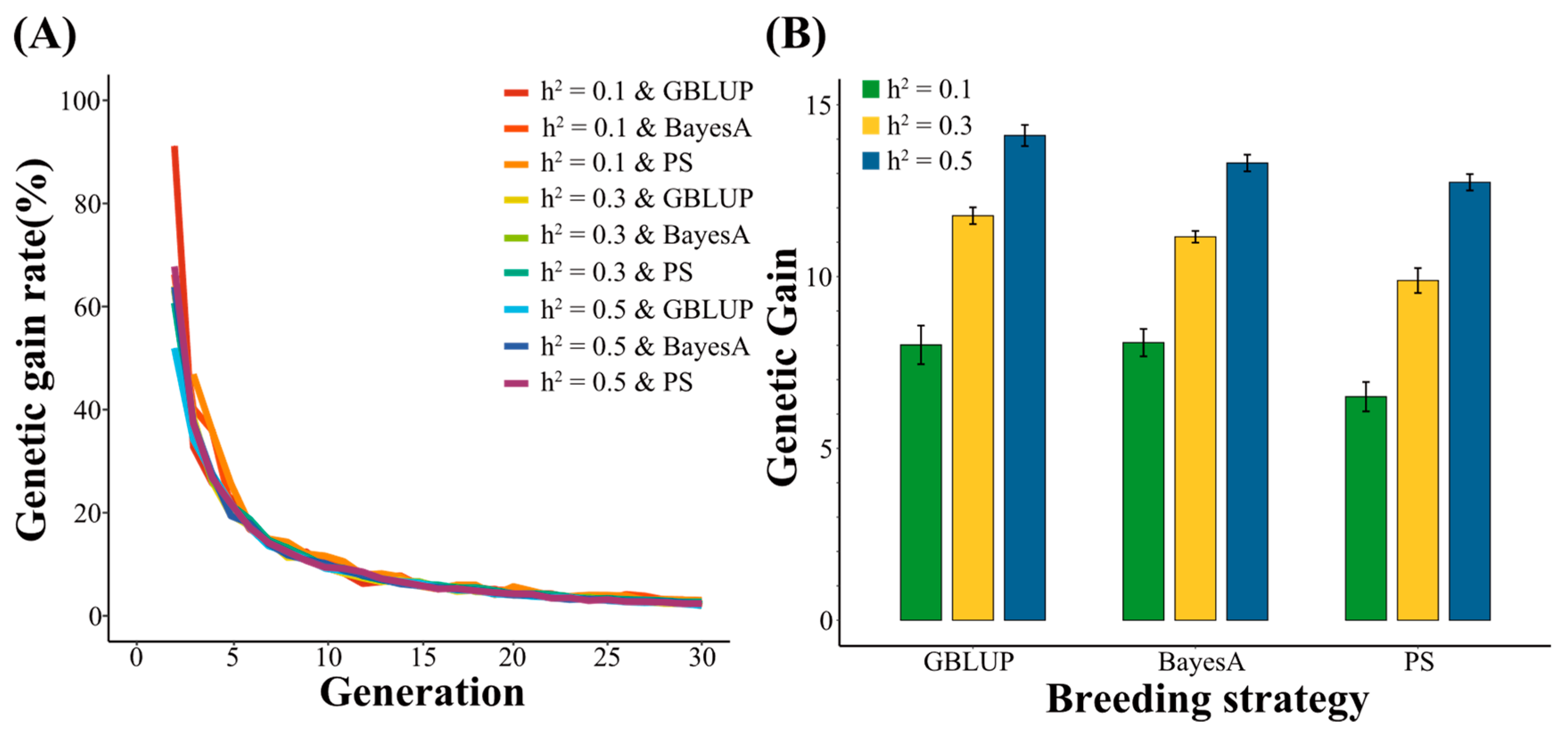
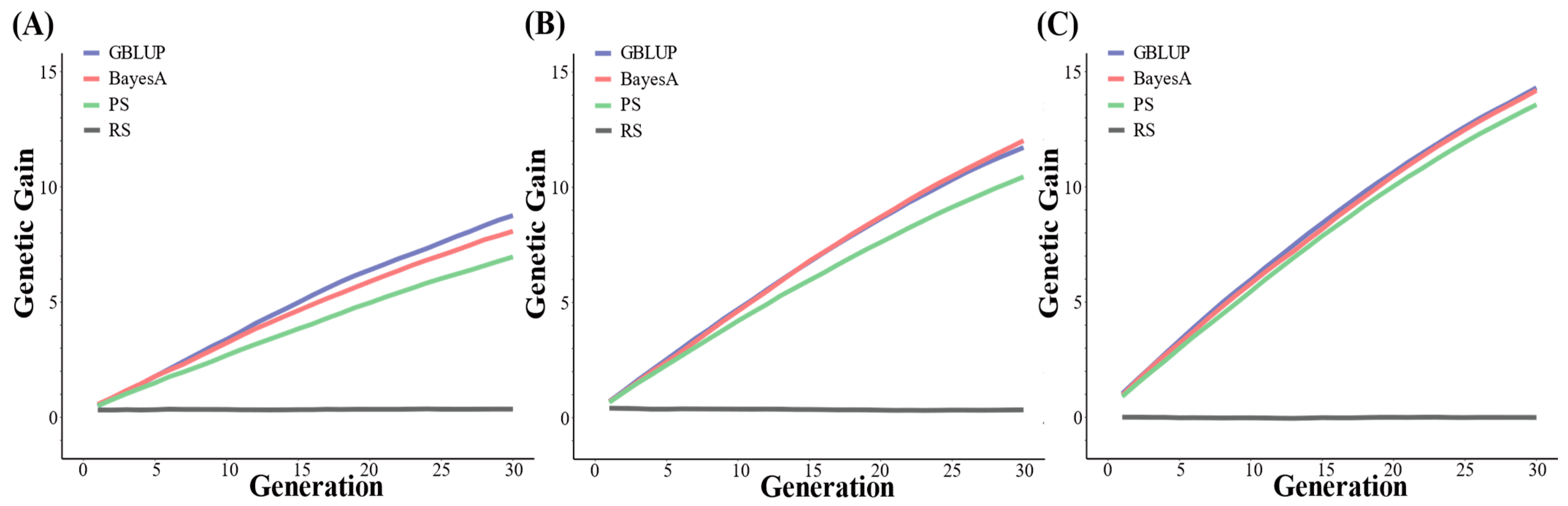
3.1. Genetic Gain Using 54 K SNPs

Using 54 K SNPs, the genetic gains gradually increase over 30 generations using three strategies—GBLUP, BayesA, and PS with the heritability of traits of 0.1, 0.3, and 0.5, respectively. In contrast, there was no significant change in the genetic gain using the RS strategy (Figure 1).
For the low heritability traits, the GBLUP and BayesA strategies showed similar effects on the genetic gain across generations. In the 30th generation, the genetic gain was 8.01, 8.08, and 6.50 using GBLUP, BayesA, and PS strategies, respectively. As for medium and high heritability trait, the GBLUP strategy showed better performance than BayesA. The genetic gains using the GBLUP strategy were 11.78 and 14.11 in the 30th generation for medium and high heritability traits, while the genetic gains using the BayesA strategy were 11.16 and 13.30.
Moreover, the genetic gain rates using the GBLUP, BayesA, and PS strategies showed a decreasing trend compared to the previous generation (Figure 2A). The genetic gain rates of the 2nd generation ranged from 51.95% to 101.28% across all scenarios, while the genetic gain rates of the 30th generation were about 2%, for all cases.
Selection strategies showed different trends across generations, along with heritability traits (Figure 2B). In general, using the GBLUP, BayesA and PS strategies, the genetic gains in the 30th generation are the highest for the high heritability traits, while the genetic gain is the lowest for the low heritability traits. Moreover, in current study, no change was observed in genetic gain using the RS strategy.

3.2. Genetic Gains Using 100 K SNPs

For 100 K SNPs, the genetic gains showed a greatly increasing trend using the GBLUP, BayesA, and PS strategies (Figure 3). For low heritability traits, the genetic gains using the GBLUP, BayesA, and PS strategies were 8.76, 8.07, and 6.96 in the 30th generation, respectively. For medium and high heritability traits, the GBLUP and BayesA strategies showed similar effects on genetic gain. The genetic gains were 11.73 and 12.02 using the GBLUP and BayesA strategies for medium heritability traits, while the genetic gains were 14.30 and 14.19 for high heritability traits. The genetic gains using the PS strategy was lower than those for the GS strategies, which were 10.45 and 13.57, respectively.
In addition, the genetic gain rate of the 2nd generation ranged from 50.47% to 71.74%, while it decreased to around 2% in the 30th generation (Figure 4A).
Using 100K SNPs, we also observed that the trait heritability has an impact on the genetic gain across generations (Figure 4B). The genetic gain in the 30th generation using the GBLUP, BayesA, and PS strategies was the highest for trait heritability at 0.5, while the genetic gain was the lowest for trait heritability at 0.1.

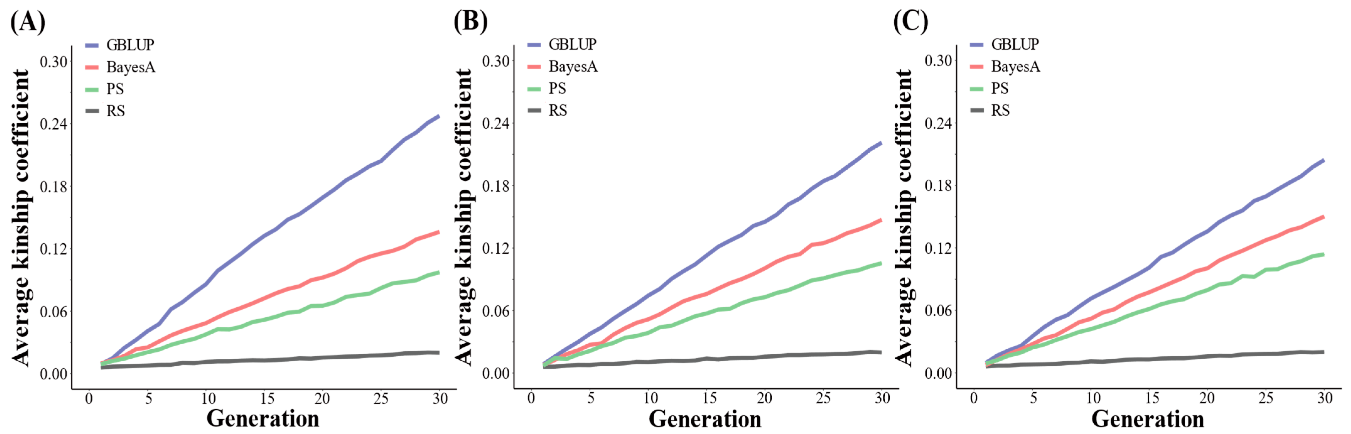
3.3. Average Kinship Coefficients Using 54 K SNPs

We estimated the average kinship coefficient across 30 generations to measure the change of inbreeding level among population. Using the 54 K SNPs, the average kinship coefficient increases to varying degrees using the GBLUP, BayesA, and PS strategies, with the exception of the RS strategy (Figure 5).
As for low, medium, and high heritability traits, the average kinship coefficients were up to 0.25, 0.22, and 0.20 using the GBLUP strategy. Using the BayesA strategy, the average kinship coefficients were 0.14, 0.15, and 0.11, respectively. The average kinship coefficients of the 30th generation using the PS strategy were 0.10, 0.11, and 0.11, which were all lower than those for the GS strategies.
The highest average kinship coefficients were obtained for trait heritability of 0.1 in the 30th generation using the GBLUP strategy, followed by heritability of 0.3, and heritability of 0.5. As for the BayesA and PS strategies, we found that the higher average kinship coefficient of the 30th generation changed along with trait heritability (Supplementary Materials Figure S2).

3.4. Average Kinship Coefficients Using 100 K SNPs

As for 100 K SNPs, we found that the change trend of the average kinship coefficients using different strategies was similar to that for 54 K SNPs. The average kinship coefficients were 0.26, 0.23, and 0.20 in the 30th generation with low, medium, and high heritability traits using the GBLUP strategy, followed by the BayesA strategy (0.13, 0.14, and 0.15), and the Ps strategy (0.09, 0.11, and 0.12). In contrast, no change for the average kinship coefficient across generations was observed using the RS strategy (Figure 6).
Using the GBLUP strategy, the higher average kinship coefficient in the 30th generation was obtained for the low heritability traits, while the higher average kinship coefficient was found for the high heritability traits using the BayesA and PS strategies (Supplementary Materials Figure S3).

3.5. Accuracy of GBLUP and BayesA Approach

We calculated the GEBVs of individuals within the population using the GBLUP and BayesA approach and derived the prediction accuracy of these two approaches (Supplementary Materials Table S1).
For the GBLUP approach, the average accuracies over 30 generations were 0.31, 0.47, and 0.57 for the low, medium, and high heritability traits using 54 K SNPs, while the average accuracies were 0.32, 0.37, and 0.58 using 100 K SNPs. For the BayesA approach, the average accuracies over 30 generations were 0.29, 0.45, and 0.57 using 54 K SNPs, while the average accuracies were 0.29, 0.46, and 0.58 using 100 K SNPs.

4. Discussion

In this study, we explored different selection strategies, trait heritability, and SNP density and evaluated their influence on the genetic gains and average kinship coefficients. We also compared the trends of genetic gain and change of the average kinship coefficients for different genetic architectures using four selection strategies. Our results showed that the GBLUP, BayesA, and PS strategies can increase the genetic gains across generations, and that these strategies also lead to different changes of kinships in the simulated populations. Our results should be helpful for designing appropriate strategies for breeding programs.

4.1. The Changes in Genetic Gain

We observed that the genetic gains vary considerably across generations using different selection strategies. As for the genetic architectures with different trait heritability, we found that the genetic gains using the RS strategy showed few changes across generations. For some generations, the average TBV of the offspring population was even lower than that of their parent population. The reason may be explained by the fact that there is no selection in RS strategy, and the gene frequency in the population remains stable [26]; thus, the trait performance in the population remains in a stable state. Similarly, the trend of kinship is stable, as there are no influence on the changes in the site frequency [6].
As for the GBLUP, BayesA, and PS strategies, the candidates were selected from the top individuals under the selection criteria; thus, the genetic performance of the offspring population is higher than that of the parents. The PS strategy showed improved performance for genetic gain in the offspring populations; however, the performance of this strategy was lower than that of the GBLUP and BayesA strategies; this finding is consistent with a previous study for dairy buffaloes [32]. Moreover, the GBLUP and BayesA strategies could help to improve genetic gain because a great amount of genomic information was used during the breeding program, supporting the previous finding that the GS promotes genetic gains by decreasing the generation interval [33], therefore the GS using genomic information can more accurately predict individual performance at a young age and shorten the generation interval [13].
A previous study has proved that higher genetic gain results mainly from higher GEBV prediction accuracy [28]. In this study, we found that the highest genetic gain was obtained using the GBLUP strategy, which was 5.41~19.08% higher than that obtained using the BaysA strategy. As for low, medium, and high heritability traits, the GEBV estimates using the GBLUP approach showed higher accuracy.
The trait heritability can influence the accuracy of the GEBV. Using the GEBV estimation approach, the higher the trait heritability, the higher the accuracy of the GEBV. This is consistent with several findings [27,34,35], as is expected from the theory in which Th2 [36] is a critical parameter (where the T is the number of the training population and h2 is the trait heritability). Thus, the accuracy of the GEBV can be influenced by trait heritability, ultimately affecting the genetic gain.
In this study, we compared the genetic gain across generations using different SNP densities, and our results suggested that SNP density also had an effect on genetic gain. Overall, the genetic gain using 100 K SNPs was higher that using 54 K SNPs (4.11% higher), relative to the two GS strategies. The SNP density is one of the most important factors affecting the accuracy of genomic prediction [37]. High SNP density can generate stronger LD across the genome; thus, the prediction accuracy is higher, as it can use more effective SNPs with LD [27,38]. Similar to our study, we also found that high SNP density yields higher prediction accuracy, leading to higher genetic gain.

4.2. Evaluating Effects on Average Kinship Coefficients

In this study, we selected candidates during the breeding process based on the goal of improving the genetic performance of the offspring. According to the “hitch-hiking effect” theory, selection can lead to an increase in the frequency of genes affecting the trait of interest and a decrease in the frequency of other alleles, thus affecting genetic diversity [39]. If genetic performance is the only focus when breeding candidates are selected, there is a high probability that individuals with good genetic performance with closer relationships will be co-selected [24], i.e., selection can lead to the increasing similarity between individuals, along with higher average kinship coefficients [40,41]. Some studies showed that selection causes the emergence of long homozygous regions in the genome, which also indicated the increased population kinship and inbreeding levels [40,42].
Using the PS strategy, we found that the average kinship coefficients were lower than those using other strategies, which was in agreement with the previous study [23]. Higher average kinship coefficients using the GBLUP and BayesA strategies may not be expected for GS. However, several studies have shown that GS may lead to an increase in the inbreeding coefficient of the offspring populations after for many generations of its application [43]. The maximization of genetic gain obtained by GS is produced through high selection intensity, which may lead to the loss of genetic diversity and the increase in inbreeding [24,44]. We found the highest average kinship coefficient using the GBLUP strategy, and the levels were much higher than those using the BayesA strategy (32.38~101.10% higher). This is likely due to the fact that the use of the BayesA approach involves a certain proportion of effective SNPs, which can effectively control the kinship of the offspring population.
We also observed that the average kinship coefficients of populations were changed according to different SNP densities. Overall, the average kinship coefficients using 100 K SNPs were slightly higher than those using 54 K SNPs. Considered in the context of genetic gain, although the populations with 100 K SNP density eventually had a higher average kinship coefficient, they also achieved higher genetic gain.
The average kinship and inbreeding levels were required to be controlled because higher inbreeding can lead to lower genetic diversity, lower response to selection, and a higher risk of homozygosity for deleterious or lethal alleles [45,46]. Several studies have confirmed that the use of GS in North American Holstein cattle populations, Jersey cattle populations, and Australian national populations has led to a rapid increase in population inbreeding levels [23,43,47]. Using simulation, our study also showed that the long-term effects of GS can lead to a rapid increase in kinship, which may lead to a rapid decline in the genetic gains.

4.3. Limitation and Prospects

Our results showed that GS can promote genetic gains across generations with different genetic architectures; however, many studies have proposed that it is important to achieve long-term and sustainable genetic gain while maintaining inbreeding levels at a low level. For instance, long-term selection, along with mating allocation based on linear programming [48] and the optimum contribution selection (OCS) method, can help to estimate the optimal number of offspring of a breeding candidate, and determine whether to select them for a breeding program [49]. These methods can efficiently control the inbreeding levels and maximize genetic gain while maintaining a certain level of genetic diversity [31].

5. Conclusions

This study showed that the GS approach can effectively promote the genetic gains of the breeding population due to the use of genomic information. The genetic gains can be affected by the selection strategy, the trait heritability, and the SNP density. The average kinship coefficient gradually increased across generations using the GS approach. The high inbreeding level may result in a reduction in inbreeding, further influencing the genetic gain rate in breeding programs. Therefore, it is necessary to improve the genetic performance while controlling the kinship among generations to maintain a long-term and sustainable genetic gain. Moreover, breeders should consider the appropriate SNP array to maximize their genetic gain and economic benefits while controlling kinship during breeding.

Supplementary Materials

The following supporting information can be downloaded at: https://www.mdpi.com/article/10.3390/agriculture12091463/s1, Figure S1: The schematic representation of simulation steps; Figure S2: The average kinship coefficient of the 30th generation based on 54 K SNPs for different heritabilities; Figure S3: The average kinship coefficient of the 30th generation based on 100 K SNPs for different heritabilities; Table S1: The prediction accuracy of the GBLUP and BayesA approach.

Author Contributions

Conceptualization, L.X., J.L. and X.Z.; methodology, X.Z. and T.Z.; software, X.Z. and Q.N.; validation, J.W. and T.W.; formal analysis, H.G.; investigation, Z.W.; resources, L.X.; data curation, J.W.; writing—original draft preparation, X.Z., T.Z. and L.X.; writing—review and editing, J.L.; visualization, T.W.; supervision, H.G.; project administration, L.X. and J.L.; funding acquisition, L.X. All authors have read and agreed to the published version of the manuscript.

Funding

This study was supported by the Agricultural Science and Technology Innovation Program of the Chinese Academy of Agricultural Sciences (CAAS-ZDRW202102, ASTIP-IAS-TS-16, and ASTIP-IAS03) and the National Beef Cattle Industrial Technology System (CARS-37). L.Y.X was supported by the Elite Youth Program of the Chinese Academy of Agricultural Sciences.

Institutional Review Board Statement

Not applicable.

Informed Consent Statement

Not applicable.

Data Availability Statement

The datasets used and analyzed during the current study are available from the corresponding author upon reasonable request (LYX). The data are not publicly available to preserve the privacy of the data.

Conflicts of Interest

The authors declare no conflict of interest.

References

  1. Meuwissen, T.H.E.; Hayes, B.J.; Goddard, M.E. Prediction of Total Genetic Value Using Genome-Wide Dense Marker Maps. Genetics 2001, 157, 1819–1829. [Google Scholar] [CrossRef]
  2. VanRaden, P. Symposium review: How to implement genomic selection. J. Dairy Sci. 2020, 103, 5291–5301. [Google Scholar] [CrossRef]
  3. Schierenbeck, S.; Pimentel, E.C.G.; Tietze, M.; Körte, J.; Reents, R.; Reinhardt, F.; Simianer, H.; König, S. Controlling inbreeding and maximizing genetic gain using semi-definite programming with pedigree-based and genomic relationships. J. Dairy Sci. 2011, 94, 6143–6152. [Google Scholar] [CrossRef]
  4. Daetwyler, H.D.; Calus, M.P.L.; Pong-Wong, R.; de los Campos, G.; Hickey, J.M. Genomic Prediction in Animals and Plants: Simulation of Data, Validation, Reporting, and Benchmarking. Genetics 2013, 193, 347–365. [Google Scholar] [CrossRef]
  5. Hickey, J.M.; Gorjanc, G. Simulated Data for Genomic Selection and Genome-Wide Association Studies Using a Combination of Coalescent and Gene Drop Methods. G3 Genes Genomes Genet. 2012, 2, 425–427. [Google Scholar] [CrossRef]
  6. Seno, L.D.O.; Guidolin, D.G.F.; Aspilcueta-Borquis, R.R.; Nascimento, G.B.D.; da Silva, T.B.R.; de Oliveira, H.N.; Munari, D.P. Genomic selection in dairy cattle simulated populations. J. Dairy Res. 2018, 85, 125–132. [Google Scholar] [CrossRef]
  7. de Rezende Neves, H.H.; Carvalheiro, R.; de Queiroz, S.A. Trait-specific long-term consequences of genomic selection in beef cattle. Genetica 2017, 146, 85–99. [Google Scholar] [CrossRef]
  8. Xu, L.; Wang, Z.; Zhu, B.; Liu, Y.; Li, H.; Bordbar, F.; Chen, Y.; Zhang, L.; Gao, X.; Gao, H. Theoretical Evaluation of Multi-Breed Genomic Prediction in Chinese Indigenous Cattle. Animals 2019, 9, 789. [Google Scholar] [CrossRef]
  9. Akanno, E.; Schenkel, F.; Sargolzaei, M.; Friendship, R.; Robinson, J. Persistency of accuracy of genomic breeding values for different simulated pig breeding programs in developing countries. J. Anim. Breed. Genet. 2014, 131, 367–378. [Google Scholar] [CrossRef]
  10. da Silva, E.D.B.; Xavier, A.; Faria, M.V. Impact of Genomic Prediction Model, Selection Intensity, and Breeding Strategy on the Long-Term Genetic Gain and Genetic Erosion in Soybean Breeding. Front. Genet. 2021, 12, 637133. [Google Scholar] [CrossRef]
  11. Burrow, H.M.; Mrode, R.; Mwai, A.O.; Coffey, M.P.; Hayes, B.J. Challenges and Opportunities in Applying Genomic Selection to Ruminants Owned by Smallholder Farmers. Agriculture 2021, 11, 1172. [Google Scholar] [CrossRef]
  12. de Roos, A.; Schrooten, C.; Veerkamp, R.; van Arendonk, J. Effects of genomic selection on genetic improvement, inbreeding, and merit of young versus proven bulls. J. Dairy Sci. 2011, 94, 1559–1567. [Google Scholar] [CrossRef]
  13. García-Ruiz, A.; Cole, J.B.; VanRaden, P.M.; Wiggans, G.R.; Ruiz-López, F.J.; Van Tassell, C.P. Changes in genetic selection differentials and generation intervals in US Holstein dairy cattle as a result of genomic selection. Proc. Natl. Acad. Sci. USA 2016, 113, E3995–E4004. [Google Scholar] [CrossRef]
  14. Samorè, A.B.; Fontanesi, L. Genomic selection in pigs: State of the art and perspectives. Ital. J. Anim. Sci. 2016, 15, 211–232. [Google Scholar] [CrossRef]
  15. Weller, J.; Ezra, E.; Ron, M. Invited review: A perspective on the future of genomic selection in dairy cattle. J. Dairy Sci. 2017, 100, 8633–8644. [Google Scholar] [CrossRef]
  16. Wiggans, G.R.; Cole, J.B.; Hubbard, S.M.; Sonstegard, T.S. Genomic Selection in Dairy Cattle: The USDA Experience. Annu. Rev. Anim. Biosci. 2017, 5, 309–327. [Google Scholar] [CrossRef]
  17. Rutkoski, J.E. Chapter Four—A practical guide to genetic gain. In Advances in Agronomy; Sparks, D.L., Ed.; Academic Press: Cambridge, MA, USA, 2019; Volume 157, pp. 217–249. [Google Scholar]
  18. Xu, Y.; Boddupalli, P.; Zou, C.; Lu, Y.; Xie, C.; Zhang, X.; Prasanna, B.M.; Olsen, M.S. Enhancing genetic gain in the era of molecular breeding. J. Exp. Bot. 2017, 68, 2641–2666. [Google Scholar] [CrossRef]
  19. Xu, Y.; Liu, X.; Fu, J.; Wang, H.; Wang, J.; Huang, C.; Prasanna, B.M.; Olsen, M.S.; Wang, G.; Zhang, A. Enhancing Genetic Gain through Genomic Selection: From Livestock to Plants. Plant Commun. 2019, 1, 100005. [Google Scholar] [CrossRef]
  20. Vanraden, P.M.; Van Tassell, C.P.; Wiggans, G.R.; Sonstegard, T.S.; Schnabel, R.D.; Taylor, J.F.; Schenkel, F.S. Invited Review: Reliability of genomic predictions for North American Holstein bulls. J. Dairy Sci. 2009, 92, 16–24. [Google Scholar] [CrossRef]
  21. Dekkers, J.C.M.; Su, H.; Cheng, J. Correction to: Predicting the accuracy of genomic predictions. Genet. Sel. Evol. 2021, 53, 81. [Google Scholar] [CrossRef]
  22. Zhu, B.; Guo, P.; Wang, Z.; Zhang, W.; Chen, Y.; Zhang, L.; Gao, H.; Gao, X.; Xu, L.; Li, J. Accuracies of genomic prediction for twenty economically important traits in Chinese Simmental beef cattle. Anim. Genet. 2019, 50, 634–643. [Google Scholar] [CrossRef]
  23. Forutan, M.; Mahyari, S.A.; Baes, C.; Melzer, N.; Schenkel, F.S.; Sargolzaei, M. Inbreeding and runs of homozygosity before and after genomic selection in North American Holstein cattle. BMC Genom. 2018, 19, 98. [Google Scholar] [CrossRef]
  24. Howard, J.T.; Pryce, J.E.; Baes, C.; Maltecca, C. Invited review: Inbreeding in the genomics era: Inbreeding, inbreeding depression, and management of genomic variability. J. Dairy Sci. 2017, 100, 6009–6024. [Google Scholar] [CrossRef]
  25. Pook, T.; Schlather, M.; Simianer, H. MoBPS-Modular Breeding Program Simulator. G3 Genes Genomes Genet. 2020, 10, 1915–1918. [Google Scholar] [CrossRef]
  26. Bastiaansen, J.W.; Coster, A.; Calus, M.P.; van Arendonk, J.A.; Bovenhuis, H. Long-term response to genomic selection: Effects of estimation method and reference population structure for different genetic architectures. Genet. Sel. Evol. 2012, 44, 3. [Google Scholar] [CrossRef]
  27. Brito, F.V.; Neto, J.B.; Sargolzaei, M.; Cobuci, J.A.; Schenkel, F.S. Accuracy of genomic selection in simulated populations mimicking the extent of linkage disequilibrium in beef cattle. BMC Genet. 2011, 12, 80. [Google Scholar] [CrossRef]
  28. Wientjes, Y.C.J.; Bijma, P.; Calus, M.P.L.; Zwaan, B.J.; Vitezica, Z.G.; van den Heuvel, J. The long-term effects of genomic selection: 1. Response to selection, additive genetic variance, and genetic architecture. Genet. Sel. Evol. 2022, 54, 19. [Google Scholar] [CrossRef]
  29. VanRaden, P. Efficient Methods to Compute Genomic Predictions. J. Dairy Sci. 2008, 91, 4414–4423. [Google Scholar] [CrossRef]
  30. Guidelines to MoBPS.pdf. Available online: https://github.com/tpook92/MoBPS/blob/master/Guidelines%20to%20MoBPS.pdf (accessed on 26 June 2022).
  31. He, J.; Wu, X.-L.; Zeng, Q.; Li, H.; Ma, H.; Jiang, J.; Rosa, G.J.M.; Gianola, D.; Tait, R.G.; Bauck, S. Genomic mating as sustainable breeding for Chinese indigenous Ningxiang pigs. PLoS ONE 2020, 15, e0236629. [Google Scholar] [CrossRef]
  32. Seno, L.; Fernández, J.; Cardoso, V.; García-Cortés, L.; Toro, M.A.; Santos, D.; Albuquerque, L.; De Camargo, G.; Tonhati, H. Selection strategies for dairy buffaloes: Economic and genetic consequences. J. Anim. Breed. Genet. 2012, 129, 488–500. [Google Scholar] [CrossRef]
  33. Schaeffer, L.R. Strategy for applying genome-wide selection in dairy cattle. J. Anim. Breed. Genet. 2006, 123, 218–223. [Google Scholar] [CrossRef] [PubMed]
  34. Bolormaa, S.; Pryce, J.E.; Kemper, K.; Savin, K.; Hayes, B.J.; Barendse, W.; Zhang, Y.; Reich, C.M.; Mason, B.A.; Bunch, R.J.; et al. Accuracy of prediction of genomic breeding values for residual feed intake and carcass and meat quality traits in Bos taurus, Bos indicus, and composite beef cattle1. J. Anim. Sci. 2013, 91, 3088–3104. [Google Scholar] [CrossRef] [PubMed]
  35. Daetwyler, H.D.; Pong-Wong, R.; Villanueva, B.; Woolliams, J.A. The Impact of Genetic Architecture on Genome-Wide Evaluation Methods. Genetics 2010, 185, 1021–1031. [Google Scholar] [CrossRef] [PubMed]
  36. Goddard, M. Genomic selection: Prediction of accuracy and maximisation of long term response. Genetica 2009, 136, 245–257. [Google Scholar] [CrossRef] [PubMed]
  37. Weigel, K.; Campos, G.D.L.; González-Recio, O.; Naya, H.; Wu, X.; Long, N.; Rosa, G.; Gianola, D. Predictive ability of direct genomic values for lifetime net merit of Holstein sires using selected subsets of single nucleotide polymorphism markers. J. Dairy Sci. 2009, 92, 5248–5257. [Google Scholar] [CrossRef]
  38. Su, G.; Brøndum, R.; Ma, P.; Guldbrandtsen, B.; Aamand, G.P.; Lund, M. Comparison of genomic predictions using medium-density (∼54,000) and high-density (∼777,000) single nucleotide polymorphism marker panels in Nordic Holstein and Red Dairy Cattle populations. J. Dairy Sci. 2012, 95, 4657–4665. [Google Scholar] [CrossRef]
  39. Maynard, J.; Haigh, J. The hitch-hiking effect of a favourable gene. Genet. Res. 2007, 89, 391–403. [Google Scholar] [CrossRef]
  40. Kim, E.-S.; Cole, J.B.; Huson, H.; Wiggans, G.R.; Van Tassell, C.P.; Crooker, B.A.; Liu, G.; Da, Y.; Sonstegard, T.S. Effect of Artificial Selection on Runs of Homozygosity in U.S. Holstein Cattle. PLoS ONE 2013, 8, e80813. [Google Scholar] [CrossRef]
  41. Kim, E.-S.; Sonstegard, T.S.; Van Tassell, C.P.; Wiggans, G.; Rothschild, M.F. The Relationship between Runs of Homozygosity and Inbreeding in Jersey Cattle under Selection. PLoS ONE 2015, 10, e0129967. [Google Scholar] [CrossRef]
  42. Bosse, M.; Megens, H.-J.; Madsen, O.; Paudel, Y.; Frantz, L.A.F.; Schook, L.B.; Crooijmans, R.P.M.A.; Groenen, M.A.M. Regions of Homozygosity in the Porcine Genome: Consequence of Demography and the Recombination Landscape. PLoS Genet. 2012, 8, e1003100. [Google Scholar] [CrossRef] [Green Version]
  43. Scott, B.; Haile-Mariam, M.; Cocks, B.; Pryce, J. How genomic selection has increased rates of genetic gain and inbreeding in the Australian national herd, genomic information nucleus, and bulls. J. Dairy Sci. 2021, 104, 11832–11849. [Google Scholar] [CrossRef] [PubMed]
  44. Curik, I.; Ferenčaković, M.; Sölkner, J. Inbreeding and runs of homozygosity: A possible solution to an old problem. Livest. Sci. 2014, 166, 26–34. [Google Scholar] [CrossRef]
  45. De Beukelaer, H.; Badke, Y.; Fack, V.; De Meyer, G. Moving Beyond Managing Realized Genomic Relationship in Long-Term Genomic Selection. Genetics 2017, 206, 1127–1138. [Google Scholar] [CrossRef] [PubMed]
  46. Akdemir, D.; Beavis, W.; Fritsche-Neto, R.; Singh, A.K.; Isidro-Sánchez, J. Multi-objective optimized genomic breeding strategies for sustainable food improvement. Heredity 2018, 122, 672–683. [Google Scholar] [CrossRef]
  47. Makanjuola, B.O.; Miglior, F.; Abdalla, E.A.; Maltecca, C.; Schenkel, F.S.; Baes, C.F. Effect of genomic selection on rate of inbreeding and coancestry and effective population size of Holstein and Jersey cattle populations. J. Dairy Sci. 2020, 103, 5183–5199. [Google Scholar] [CrossRef]
  48. Carthy, T.; McCarthy, J.; Berry, D. A mating advice system in dairy cattle incorporating genomic information. J. Dairy Sci. 2019, 102, 8210–8220. [Google Scholar] [CrossRef]
  49. Meuwissen, T.; Sonesson, A.K. Maximizing the response of selection with a predefined rate of inbreeding: Overlapping generations. J. Anim. Sci. 1998, 76, 2575–2583. [Google Scholar] [CrossRef]
Figure 1. Genetic gains across 30 generations using 4 strategies with low, medium, and high heritability traits based on 54 K SNPs. (A) Genetic gains for trait heritability of 0.1. (B) Genetic gains for trait heritability of 0.3. (C) Genetic gains for trait heritability of 0.5.
Agriculture 12 01463 g001
Figure 2. (A) Genetic gain rates across 30 generations for all scenarios using 54 K SNPs. (B) The genetic gains of the 30th generation based on 54 K SNPs for different heritabilities.
Agriculture 12 01463 g002
Figure 3. Genetic gains across 30 generations using 4 strategies with low, medium, and high heritability traits based on 100 K SNPs. (A) Genetic gains for trait heritability of 0.1. (B) Genetic gains for trait heritability of 0.3. (C) Genetic gains for trait heritability of 0.5.
Agriculture 12 01463 g003
Figure 4. (A) Genetic gain rates across 30 generations for all scenarios using 100 K SNPs. (B) The genetic gains of the 30th generation based on 100 K SNPs for different heritabilities.
Agriculture 12 01463 g004
Figure 5. Average kinship coefficients of 4 strategies with low, medium, and high heritability traits using 54 K SNPs. (A) Average kinship coefficients for trait heritability of 0.1. (B) Average kinship coefficients for trait heritability of 0.3. (C) Average kinship coefficients for trait heritability of 0.5.
Agriculture 12 01463 g005
Figure 6. Average kinship coefficients of 4 strategies with low, medium, and high heritability traits using 100 K SNPs. (A) Average kinship coefficients for trait heritability of 0.1. (B) Average kinship coefficients for trait heritability of 0.3. (C) Average kinship coefficients for trait heritability of 0.5.
Agriculture 12 01463 g006
Table 1. Different genetic architecture of HP.
ScenarioTrait HeritabilitySNP Density
10.154 K
20.1100 K
30.354 K
40.3100 K
50.554 K
60.5100 K
Publisher’s Note: MDPI stays neutral with regard to jurisdictional claims in published maps and institutional affiliations.

