Determination Method of Core Parameters for the Mechanical Classification Simulation of Thin-Skinned Walnuts

Abstract

Simulation can be used to visualize the mechanical classification of walnuts. It can collect microscopic information about walnuts in the classification roller and guide its optimization design. In this process, simulation parameters are essential factors that ensure the effectiveness of the simulation. In this study, the crucial parameters of thin-skinned walnut particles in classification simulation were determined by combining the discrete element method (DEM) and physical tests. Firstly, the moisture content, shear modulus, stacking angle, and some contact parameters in the shell and kernel were obtained by drying test, compression test, cylinder lifting test, and physical test of contact parameters, respectively. A walnut model was constructed using reverse modeling technology. Then, the ranges of the rest contact parameters were determined using simulation inversion based on the Generic EDEM Material Model database. Second, the parameters significantly influencing the stacking angle were screened via the Plackett–Burman test using contact parameters as factors and stacking angle as the index. The results revealed that the walnut–walnut static friction coefficient, walnut–walnut rolling friction coefficient, and walnut–steel plate static friction coefficient significantly affect the stacking angle. The steepest ascent experiment produced the optimal value intervals of crucial parameters. Besides, a quadratic regression model of important parameters was built using the Box–Behnken test to achieve the optimal parameter combination. The stacking and classification experiments verified that the stacking angle and morphology are mostly similar under calibration parameters without any considerable differences. The relative error was only 0.068%. Notably, the relative error of the average staying time of walnut in the classification roller was 0.671%, and the dimensionless distribution curves of stay time were consistent. This study provides technological support to the simulation analysis of walnut classification and recommends novel methods and references to determine the parameters of other shell materials.

1. Introduction

Walnut has extremely high edibleness and medicinal value and is one of the major nuts worldwide [1]. During post-harvest processing, the sales of walnuts that are graded according to size can attain higher values. Besides, size-based walnut classification is essential for breaking shells and collecting kernels in the shell-breaking device with fixed clearance [2]. However, wrong categorization (some small walnuts are mixed in with the big ones following classification) poses a universal challenge in the existing walnut classification devices [3]. The conventional “black box” analytical methods cannot identify the causes of wrong classifications (insufficient classification precision) from the microscopic level, thereby restricting the optimization design of relevant devices to some extent. Therefore, it is urgent to determine the walnut’s intrinsic and contact parameters, explore the fundamental movement laws during walnut classification according to visualization characteristics of simulation, and guide the walnut classification process.

Walnut classification is primarily investigated through trial and error [4]. However, this method is time-consuming, labor-intensive, and cannot accurately and thoroughly capture the complicated stress and movement characteristics of walnuts in the classification roller. The discrete element method (DEM) takes a shorter time for optimization design, can save costs, and monitors and extracts real-time information on particles. It has been applied preliminarily in the size-based classifications and shell-kernel separation of walnut. Notably, it has produced some beneficial results [5,6]. However, all the contact parameters in previous simulations were from materials with similar properties to walnut. Contact parameters and mechanical properties of materials vary with categories and species [7]. The accuracy of simulation parameters and model authenticity directly determine the effectiveness of the simulation analysis [8]. In recent years globally, scholars have investigated the critical simulation characteristics (intrinsic parameters and contact parameters) of materials, such as crop seeds, soil, fertilizers, and straws, among others. Zhou et al. [9] developed a simulation model of maize particles using the stacked sphere method. Importantly, they calibrated the seed parameters using the stacking angle test and the “self-flow screening” test. Yan et al. [10] simplified the soil particle model into small and simple overlapping spheres. Furthermore, they verified the accuracy of the calibration parameters using a straight shear test. Xie et al. [11] combined physical and simulation tests to achieve the best parameters for simulation test materials of organic fertiliser granules. Fang et al. [12] established a simulation model of corn stover pellets using 3D modeling and the multi-ball filling method. They calibrated the stover simulation parameters based on the response surface method. Nevertheless, it is unfortunate that the parameter calibration of thin-skinned walnuts has yet to be reported. More importantly, many scholars have achieved approximate ranges of contact parameters of materials whose direct evaluation via the Generic EDEM Material Model (GEMM) database is challenging [13,14]. The universality of these ranges is still up for comprehensive discussion [15]. Hence, an inversion method based on DEM was proposed to measure the ranges of contact parameters with insufficient reference data. Investigating walnut classification based on the discrete element simulation has a huge significance. It can provide method references to calculate the ranges of contact parameters in simulation with insufficient reference data of shell materials.

Based on the background presented above, the research objectives of this study are as follows. (1) The ranges of intrinsic parameters (moisture content, density, and shear modulus) and measurable contact parameters (walnut–steel plate collision recovery coefficient, walnut–steel plate static friction coefficient, and walnut–walnut collision recovery coefficient) of walnuts were established via a physical test. Meanwhile, the stacking angle of walnuts was calculated by combining the cylinder lifting stacking test and MATLAB image processing technology. (2) A walnut simulation model was constructed via the three-dimensional scanning reverse modeling technique. The ranges of difficult-to-measure contact parameters (walnut–walnut static friction coefficient, walnut–walnut rolling friction coefficient, and walnut–steel plate rolling friction coefficient) were determined via simulation inversion based on the GEMM database. Subsequently, the Plackett–Burman test, ascent experiment, and Box–Behnken test were conducted with the Design Expert software using the measured stacking angle as the response value to calibrate the contact parameters of the walnut simulation. (3) The applicability of calibration results was verified by the cylinder lifting test and classification test to deduce the movement laws of walnuts in the classification process and provide theoretical references for the optimization of the classification machine.

2. Materials and Methods

2.1. Acquisition of Walnut Intrinsic Parameters

The experimental samples for this study were collected from the walnut garden in Wensu County, Aksu, which is one of China’s major high-quality walnut production areas. After removing the green peel and surface cleaning, the walnut samples were dried in the shadow for half day and again dried for four to six days under natural conditions with a daily average temperature of 30 °C. When the dry basis moisture content in the walnut was lower than 8%, the walnut samples were stored at a constant temperature (23 °C) and cold humidity storage (humidity of 45%). In the experiment, walnuts with normal appearances and no apparent defects or cracks were selected as test samples.

2.1.1. Moisture Content and Density Tests of Walnuts

Because the moisture content is closely related to the stacking angle and mechanical properties of materials, the moisture content of walnut samples was tested by the drying method according to GB50093—2016 Food Safety National Standards for Water Test in Foods. The calculation formula [16] is expressed as follows:

$$MC=\frac{M-Me}{Me}\times 100\%$$

(1)

where MC is the dry basis moisture content, M is the initial quality of walnut samples, and M_e is the mass of the dry sample.

In total, 20 walnuts with full kernels and good sealing performances were selected randomly. After sealing processing, the density was measured using the drainage method proposed by C. González-Montellano [17].

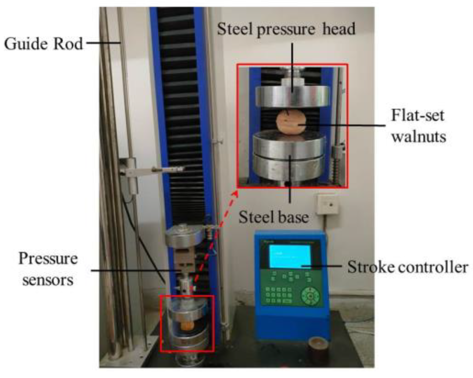
2.1.2. Geometric Size and Shear Modulus Test of Walnuts

A total of 400 walnuts were chosen randomly from test materials. The three-dimensional geometric dimension (W [axial] × L [longitudinal] × H [shortest axis]) of walnuts was measured using a Vernier caliper with an accuracy of 0.02 mm (Figure 1). Then, the average three-dimensional geometric dimension was calculated.

In total, 100 walnuts without cracks and openings were randomly selected from the test samples for size measurement and numbered accordingly. The corresponding three-dimensional geometric dimensions were also documented. A walnut was placed at the right center of the pressure head of the universal material testing machine (WD-D3-7). Then, it was compressed along its axial direction (Figure 2). It was a quasi-static compression, and the descending rate of the head was 0.02 mm/s [18].

The formula of elastic modulus can be deduced from the Hertz formula [19]:

$$E=\frac{0.388F\left(1-{\mu }^2\right)}{D^{3/2}}{\left[K_U{\left(\frac{1}{R_U}+\frac{1}{R_U^{\prime }}\right)}^{1/3}+K_L{\left(\frac{1}{R_L}+\frac{1}{R_L^{\prime }}\right)}^{1/3}\right]}^{3/2}$$

(2)

where E is the elastic modulus of the walnut (Pa); F is the static load applied onto the walnut (N); D is the deformation volume of walnuts (mm); µ is the Poisson’s ratio of walnuts, and it is determined as 0.3 [20]. R_U and R′_U are the minimum and maximum radii of curvature of the upper contact surface of walnuts (mm), respectively. R_L and R′_L are the minimum and maximum radii of curvature of the lower contact surface of walnuts (mm), respectively. K_U and K_L are the principal radii of curvature decision constants (by calculating cosθ, these two parameters can be checked in the standards of ASAE S368.4DEC2000 [R2008]). Based on the Hertz contact theory, the following calculations were made: cosθ = (1/R_U − 1/R′_U)/(1/R_U + 1/R′_U), where θ is the included angle between the upper walnut surface and head at the contact point (°).

Because the radii of curvature of the contact surface between the walnut and the head are almost similar, Equation (3) can be simplified as follows:

$$E=\frac{0.388F\left(1-{\mu }^2\right)}{D^{3/2}}{\left[2K_U{\left(\frac{1}{R_U}+\frac{1}{R_U^{\prime }}\right)}^{1/3}\right]}^{3/2}$$

(3)

where R_U = (H²/4 + W²)/2W and R′_U = (L²/4 + W²)/2W.

The calculation formula of shear modulus (G) is expressed as follows:

$$G=\frac{E}{2(1+\mu )}$$

(4)

where G is the shear modulus of walnuts (Pa); E is the elasticity modulus of walnuts (Pa); and μ is the Poisson’s ratio of walnuts.

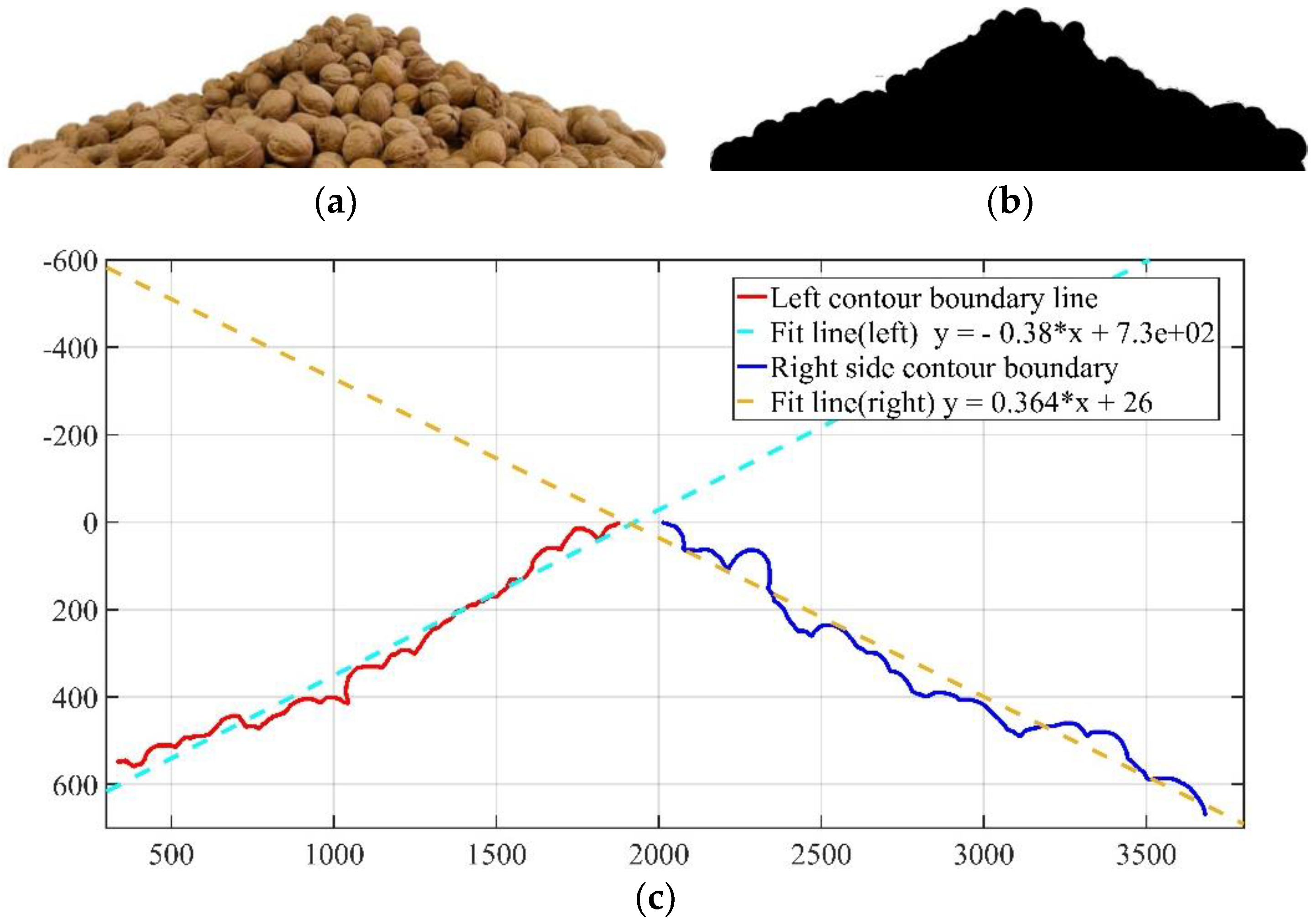
2.1.3. Physical Test of the Stacking Angle of Walnuts

Many complicated movement forms are present during the stacking of granular materials. They can efficiently characterize the scattering, flowing, and frictional features of materials and are highly significant for the harvest, storage, and transportation of materials [21]. The test methods of the stacking angle include the funnel, plate drawing, and cylinder lifting methods, among others [22]. Among them, the cylinder lifting method is easy to use and can better reflect walnuts’ scattering performances. The cylinder was made of steel with a diameter/height ratio of 1:3 (d₀ = 20 cm, h₀ = 60). Walnuts with random sizes were fed into the cylinder, which was lifted vertically at the rate of 0.05 m/s. After stabilizing the stacking slope, the front views of walnut stalking were captured at the fixed position (Figure 3a). A total of ten tests were performed. Subsequently, the walnut pile images were normalized, and a single-size boundary profile of the stacking angle [23] was extracted. The slope (k) was achieved by fitting the profiles based on the least squares method (Figure 3). Moreover, the stacking angle of the walnuts was obtained as follows:

$$\theta =\frac{\arctan \left|k\right|\times 180°}{\pi }$$

(5)

Because the included angles between the left and right slopes of the walnut pile with the horizontal surface were slightly different, the left and right boundary profiles of the walnut pile were fitted in this experiment, respectively. Finally, the mean value was selected.

2.2. Acquisition of Measurable Contact Parameters of Walnuts

Walnuts (W = 34.6 ± 1 mm, L = 40.2 ± 1 mm, H = 33.3 ± 1 mm, weight = 12 ± 0.5 g) with a size similar to the mean dimension, standard morphology, and good sealing performances were selected in the investigation of measurable contact parameters.

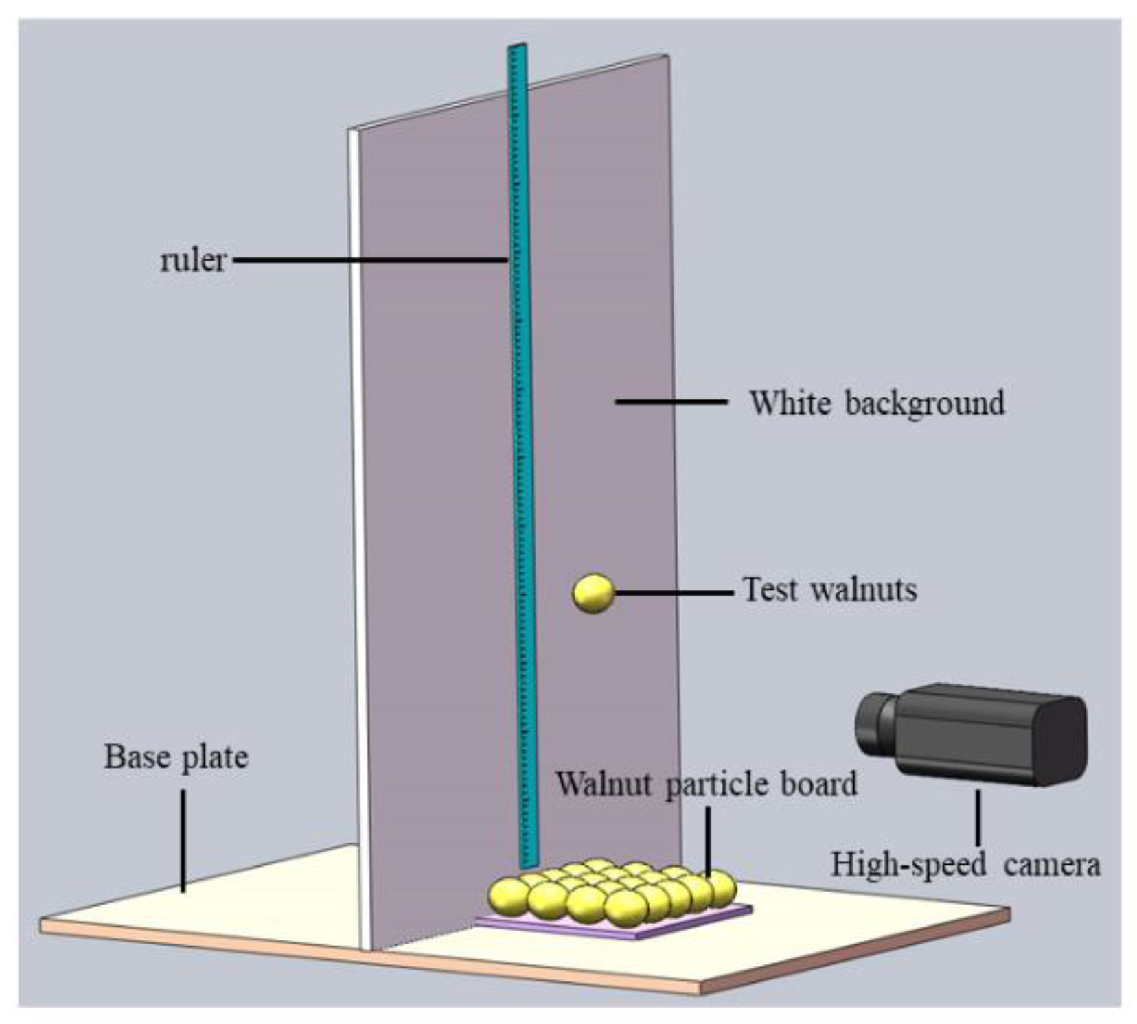
2.2.1. Collision Recovery Coefficient Test of Walnuts

The walnut–walnut collision recovery coefficient (e_pp) and walnut–steel plate collision recovery coefficient (e_ps) was evaluated using the particle–plate collision test. Before the test, 20 walnuts with generally consistent dimensions were bonded onto the steel plate to create a piece of particle board. A test platform was constructed at the same time (Figure 4). The walnut samples fell from a particular height, and their releasing height (h₁) and the maximum bouncing height (h₂) on the particle board were recorded using a high-speed camera. The results of several pre-tests revealed that walnuts might break upon impact if the falling height is too high, influencing test results’ accuracy. If the falling height is too low, the bouncing displacement of walnuts is relatively small, which is disadvantageous for measurement. Finally, h₁ was determined as 40 cm. Three walnuts were selected, and ten tests were conducted.

It is assumed that walnuts only face the gravitational force in the falling process (the air drag force is ignored). According to the theorem of kinetic energy and the definition of collision recovery coefficient, the following expression can be obtained [24]:

$$e=\frac{\left|v_2\right|}{\left|v_1\right|}=\sqrt{\frac{h_2}{h_1}}$$

(6)

where v₁ is the instantaneous normal velocity of collision at the contact point (m/s); v₂ is the instantaneous normal velocity of separation at the contact point (m/s); h₁ is the initial height of a freely falling body before collision (mm); and h₂ is the maximum height following collision rebounding (mm). The particle board must be replaced with a piece of steel plate to measure e_ps.

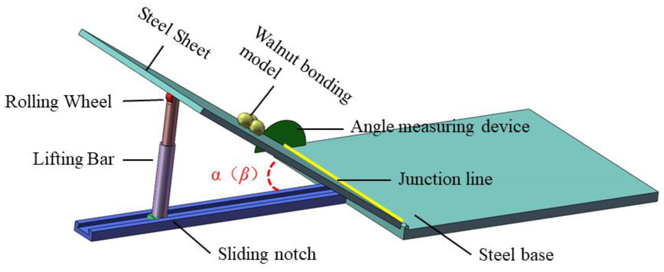
2.2.2. Test of Walnut–Steel Plate Static Friction Coefficient (μ_s,ps)

μ_s,ps was tested using the independently built slope (Figure 5). Nine walnuts were chosen in this experiment, and three walnuts with consistent dimensions were bonded together to avoid the errors caused by the rolling of walnuts. Three groups of experiments were conducted, and ten tests were performed on each group.

The walnut bonding model was placed onto the steel plate at the beginning of the experiment, and one end of the steel plate was lifted slowly. The rotation was stopped when the walnuts began to slide. At this moment, the included angle (α) between the steel plate and the horizontal surface was measured. According to the stress analysis, the following expression is obtained:

$$\mu s,ps=\frac{f}{N}=\frac{G\sin \alpha }{G\cos \alpha }=\tan \alpha$$

(7)

2.2.3. Test of Walnut–Steel Plate Rolling Friction Coefficient (μ_r,ps)

Section 2.2.2 describes the test platform in detail. The walnuts rolled downwards from a fixed point on the slope (dip angle = β) at the initial rate of 0. The straight distance between this fixed point and the steel base was X₀. Under the action of rolling friction, walnuts stopped at a distance (x) after rolling on the horizontal surface. The results of numerous pre-tests revealed that the trajectory of walnuts was a curve when X₀ was too high, thus influencing experimental results. x is also very small when X₀ is too small, which is disadvantageous in measuring x. Walnuts may “jump” if β is too high, but they cannot roll on the slope if β is too small. Finally, the following values were determined: β = 9° and X₀ = 80 cm. Following rigorous measurement and screening, 100 walnuts with typical characteristics and medium-level size were selected, and three walnuts were randomly chosen from among them. Each test was repeated by ten times. Walnuts are assumed to be ideal ellipsoids, and rolling was considered when sliding effects were not considered. It is easy to obtain the following expression from the conservation of energy [25]:

$$mgX0\sin \beta ={\mu }_{r,ps}mg\left(\cos \beta X0+x\right).$$

(8)

2.3. Construction of the Simulation Model and Acquisition of Unmeasurable Contact Parameters of Walnuts

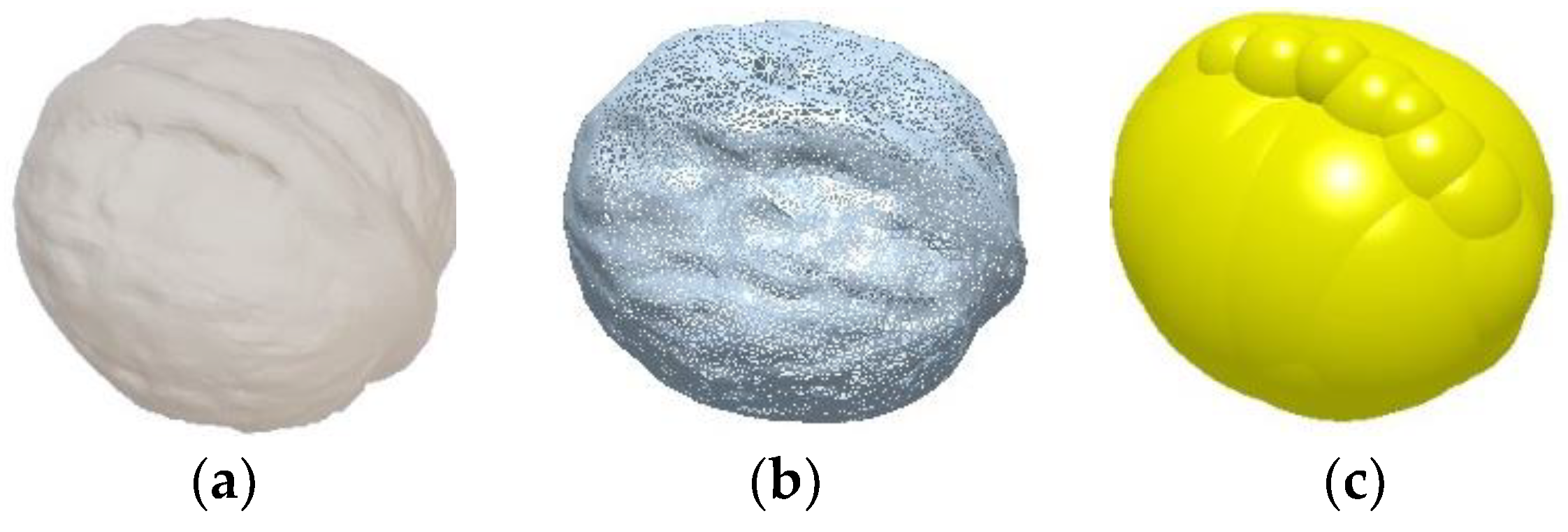
2.3.1. Discrete Element Modeling of Walnut Particles based on Three-Dimensional Scanning

Walnut has quite an irregular appearance; hence, the traditional simplified spherical modeling method cannot accurately reproduce its fundamental features. In this test, three-dimensional scanning technology was applied to effectively extract the dimension profile of walnuts. The mean three-dimensional geometric dimension of walnuts was measured as W = 34.6 mm, L = 40.2 mm, and H = 33.3 mm. The 3D scanning model of walnuts was scaled to the average walnut dimension by SolidWorks and then stored in the STL format. Subsequently, EDEM was input for particle filling. If the particle radius of filling spheres were smaller, then the quantity of filling spheres would be higher. Moreover, it could better approach the natural morphology of walnuts. However, this may affect the speed of simulation calculation and occupy computer storage resources. By carefully considering the above factors, it was finally determined that the model comprised 44 spheres of different sizes (Figure 6). This model is closer to reality and ensures a good calculation speed. It can eliminate the errors of simulation tests to some extent. It makes early preparations for the parameter calibration of DEM and classification simulation of walnuts.

2.3.2. Construction of the Simulation Model and Parameter Setting

A simulation model was constructed using SolidWorks. Subsequently, the model in the IGS format was input into EDEM. The cylinder and steel plate models were set to steel simultaneously. With respect to the intrinsic parameters, the Poisson’s ratio, density, and shear modulus were 0.28, 7.85 × 10³ kg/m^3, and 8.2 × 10¹⁰ Pa, respectively [26]. According to the characteristics of walnuts, the Hertz–Mindlin (no slip) contact model was selected in this study, and the gravity was Z = −9.81 m/s². A particle plant was set according to walnuts’ particle size distribution range. It had a dynamic particle production method. The total number of particles and the generation rate were 620 and 6.2 × 10³ psc/s, respectively. The time step in the calculation was set to 20% of Rayleigh’s time step. The data storage interval was 0.01 s, and the grid size was thrice the minimum particle radius. After stabilizing the number of simulation particles, the cylinder was lifted towards the +Z direction at the rate of 0.05 m/s, thus forming a stable particle pile (Figure 7).

2.3.3. Simulation Inversion Experiment

Walnut has unique structures and complicated appearances. Reference data are insufficient to determine the measurement ranges of contact parameters. In this experiment, an inversion method identified the ranges of contact parameters that cannot be measured directly by using the recommended value of the EDEM official database as a reference and simulation stacking results as orientation. It was used to determine the walnut–walnut static friction coefficient (μ_s,pp), walnut–walnut rolling friction coefficient (μ_r,pp), and walnut–steel plate rolling friction coefficient (μ_r,ps). Specifically, the standard parameter combination was first obtained. The measurable parameters of the physical test used the test results in Section 2.2.1 and Section 2.2.2 Parameters that cannot be measured directly were set with references to the GEMM database. One parameter that cannot be measured directly was selected as the variable, increasing from 0 to 1.0 successively. The increasing amplitude was 0.1, and the rest parameters were kept constant. The rest can be conducted in the same way.

3. Results and Discussion

3.1. Physical Test Results

Table 1. Parameter lists of the Physical test measurement results.

Parameters	Value
Dry basis moisture content of walnut kernel /%	3.53 ± 0.29
Dry basis moisture content of walnut shells/%	6.51 ± 0.34
Density of walnuts/kg × m−3	5.27 × 102 ± 0.26 × 102
Shear modulus of walnuts/Pa	2.4 × 107 ± 0.46 × 107
Walnut–walnut restitution coefficient	0.14~0.46
Walnut–steel plate restitution coefficient	0.16~0.48
Walnut–steel plate static friction coefficient	0.16~0.36
Walnut–steel plate rolling friction coefficient (under the ideal state)	0.093~0.119

demonstrates the results of tests presented in Section 2.1.1, Section 2.1.2 and Section 2.2.3.

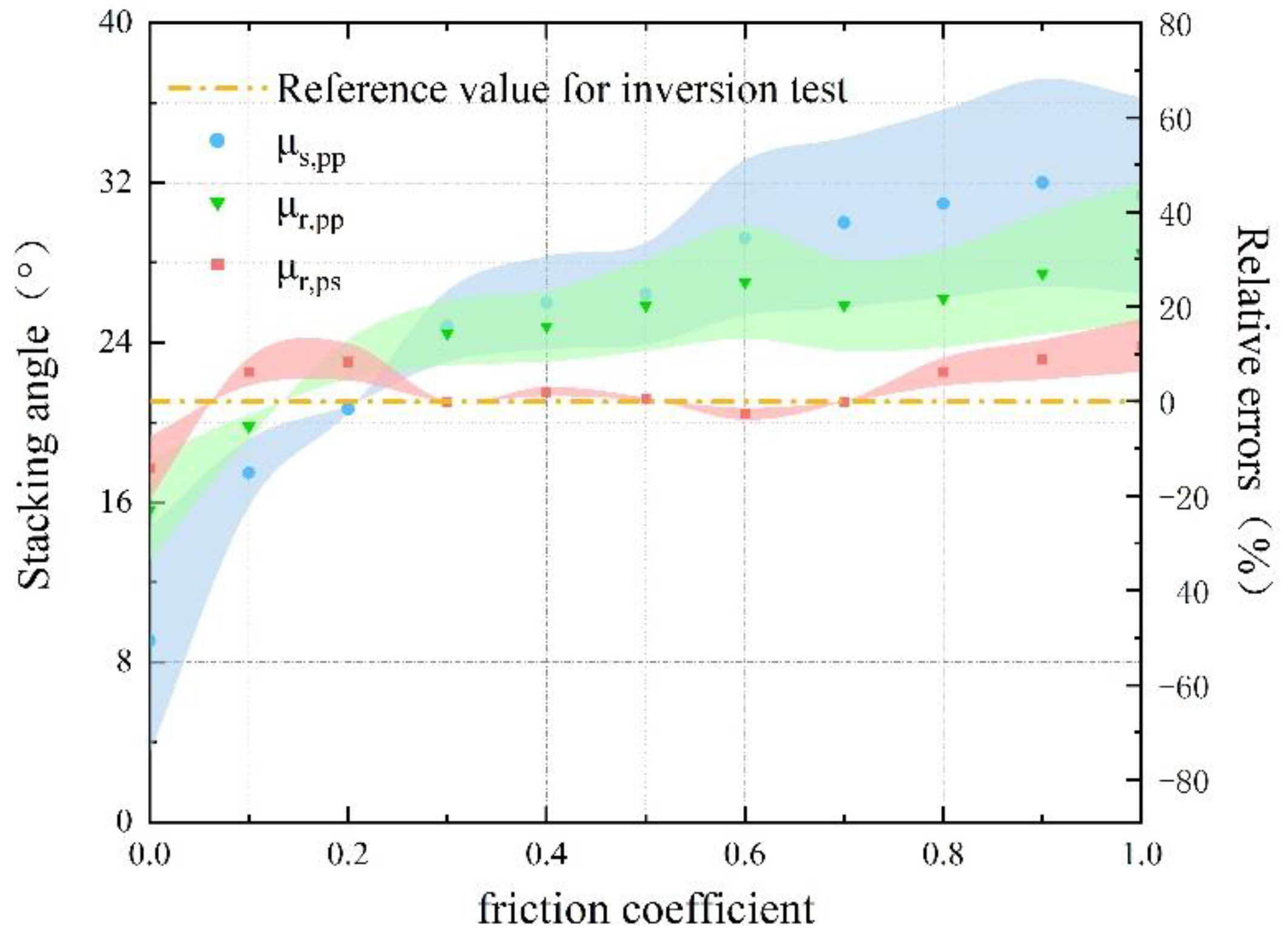
3.2. Unmeasurable Contact Parameters (μ_r,pp, μ_s,pp, μ_r,ps)

The contact parameters that cannot be measured directly were obtained according to the test presented in Section 2.3.3 (Figure 8). The simulation stacking angle increases with the increase in μ_s,pp and μ_r,pp. Its error with the standard stacking angle (21.06°) first decreases and then increases. The range of the friction coefficient failing to reach the actual stacking angle and the range of friction coefficient with significant differences between the stacking slope profile and the actual slope profile were eliminated. The following values were determined: μ_s,pp = 0.1~0.3 and μ_r,pp = 0~0.2. In contrast, the simulation stacking angle increases and then fluctuates with the increase in μ_r,ps. Its error with the standard stacking angle decreases then increases, and finally fluctuates. This parameter affects the scattering of walnuts on the steel plate. It determines the rolling distance of walnuts on the steel plate surface following their elimination from the bottom of the cylinder [27]. By comparing the pile tail morphology in the front view of the simulated and actual pile and the particle scatter distribution condition in the top view of the pile. With regard to Section 2.2.3 and Section 2.3.3, μ_r,ps was determined as 0~0.12.

3.3. Parameter Calibration

Based on the abovementioned tests, the ranges of intrinsic parameters, measurable contact parameters, and degrees of simulation contact parameters of walnuts that cannot be measured directly were obtained. Because of the complicated appearances and relatively large ranges of coefficients of walnuts, an experiment was designed using the Design Expert software to swiftly and accurately determine the simulation contact parameters.

3.3.1. Plackett–Burman Test

The mean stacking angle was acquired from the actual cylinder lifting test and used as the response value. The Plackett–Burman test was designed by the Design Expert software to screen the factors that significantly influence the stacking angle from six contact parameters. The parameters requiring calibration were expressed by A~F (

Table 2. Parameter lists of the Plackett–Burman test.

Simulation Parameters	Level			Label
	−1	0	1
Walnut–walnut restitution coefficient	0.14	0.3	0.46	A
Walnut–walnut static friction coefficient	0.1	0.2	0.3	B
Walnut–Walnut rolling friction coefficient	0	0.1	0.2	C
Walnut–steel plate restitution coefficient	0.16	0.32	0.48	D
Walnut–steel plate static friction coefficient	0.16	0.26	0.36	E
Walnut–steel plate rolling friction coefficient	0	0.06	0.12	F

).

The simulation test has inconsistent stacking angles on left and right slopes. In order to decrease errors, the least squares method was used to extract the left and right slopes of the simulation stacking angle based on MATLAB and select its mean value. The specific test procedure is explained in Section 2.1.3.

Table 3. Plackett–Burman test design and results.

No.	A	B	C	D	E	F	Stacking Angle θ/(°)
1	−1	1	−1	1	1	−1	10.65
2	1	1	1	−1	−1	−1	15.38
3	1	−1	1	1	−1	1	9.09
4	1	−1	1	1	1	−1	14.84
5	−1	−1	−1	−1	−1	−1	3.21
6	−1	−1	−1	1	−1	1	5.68
7	1	1	−1	1	1	1	21.06
8	1	1	−1	−1	−1	1	9.09
9	−1	1	1	1	−1	−1	18.78
10	−1	1	1	-1	1	1	39.18
11	1	−1	−1	−1	1	−1	1.23
12	−1	−1	1	−1	1	1	20.56
13	0	0	0	0	0	0	21.01
14	0	0	0	0	0	0	21.21
15	0	0	0	0	0	0	21.06

presents the Plackett–Burman test design and results.

Table 4. Parameter significance test of the Plackett–Burman test.

Source	Sum of Mean Squares	Degree of Freedom	Mean Square	F-Value	p-Value	Significance
Model	1052.64	6	175.44	6.2	0.011 *	—
A	62.43	1	62.43	2.2	0.176	5
B	295.32	1	295.32	10.43	0.012 *	2
C	373.08	1	373.08	13.18	0.007 **	1
D	6.09	1	6.09	0.22	0.655	6
E	178.56	1	178.56	6.31	0.036 *	3
F	137.16	1	137.16	4.84	0.059	4

Notes: ** means that this term is highly significant (p < 0.01), and * means that this term is extremely significant (0.01 < p < 0.05), hereinafter inclusive.

shows that C exerts the most significant effect on the stacking angle of walnuts, followed by B, E, F, A, and D successively. Among them, F exerts an insignificant impact on the stacking angle of walnuts. This outcome may occur because F primarily impacts the scattering characteristics of particles at the edges of the particle pile. When F is small, the particles scatter well and are relatively discrete at the edges of the pile. The variations of F can significantly affect the stacking angle. With the increase in F, particles are more concentrated on the steel plate at the edges of the pile. As a result, the effects of F on the stacking angle decrease gradually and tend to be insignificant. Consequently, the effects of F on the stacking angle are generally negligible. Among them, A and D do not significantly affect the stacking angle. The reason may be that the steel cylinder is lifted slowly during the stacking process, the collision energy between walnuts and between walnuts and steel plates is low, and their changes have no significant effect on the stacking angle. Hence, A and D cannot be calibrated via the stacking test, and the means were collected in the follow-up test. B and E significantly affect the stacking angle, and C exhibits highly significant effects. These three parameters must be further analyzed and calibrated.

3.3.2. Steepest Ascent Experiment

Based on the Plackett–Burman test, the steepest ascent experiment was conducted on three significance parameters (B, C, and E) to quickly narrow the ranges of significance parameters. During the parameter setting, the insignificant parameters A, D, and F were set at the 0 levels [11,28]. Significance parameters were kept at the step length of 0.04.

Table 5. The steepest ascent experiment scheme and results.

No.	Parameters			Stacking Angle θ/(°)
	B	C	E
1	0.1	0	0.16	5.23
2	0.14	0.04	0.2	11.86
3	0.18	0.08	0.24	17.74
4	0.22	0.12	0.28	26.57
5	0.26	0.16	0.32	33.02
6	0.3	0.2	0.36	35.75

shows the test results. The simulation stacking angle increases with the increase in B, C, and E, and its relative error with the physical stacking angle first decrease and then increases. The relative error of Test 3 is the lowest (11.79%). Hence, parameters in Test 3 were chosen at the 0 levels of the Box–Behnken test. The parameters of Test 2 and Test 4 were set at the high (+1) and low (−1) levels, respectively. For instance, B takes 0.14~0.22, C takes 0.04~0.12, and E takes 0.2~0.28 as the optimal range of values for the three significance parameters.

3.3.3. Box–Behnken Test

Based on the steepest ascent experiment results, the Box–Behnken module of the Design Expert software was applied to design the experiment. B, C, and E were used as factors, whereas the simulation of the stacking angle was used as the index. Effects of quadratic terms of three factors and the pairwise interaction terms of B, C, and E on the stacking angle were also investigated.

Table 6. Box–Behnken test results.

No.	Parameters			Stacking Angle θ/(°)
	B	C	E
1	0	0	0	17.74
2	−1	0	1	17.22
3	0	0	0	16.96
4	1	0	−1	17.74
5	1	1	0	20.56
6	0	1	−1	15.91
7	0	0	0	16.96
8	0	−1	−1	11.86
9	0	−1	1	18.52
10	0	1	1	22.29
11	−1	1	0	16.44
12	−1	0	−1	15.11
13	0	0	0	17.48
14	0	0	0	18.34
15	−1	−1	0	13.22
16	1	0	1	24.7
17	1	−1	0	18.26

shows the experimental design and results.

According to the test results in Table 6, a quadratic regression model between three variables and simulation stacking angle was constructed by the Design Expert software. The quadratic polynomial equation was expressed as follows:

$$\begin{array}{c}\theta =+17.34+2.41\ast B+1.49\ast C+2.59\ast E\\ -0.23\ast BC+1.21\ast BE-0.07\ast CE\\ +0.66\ast B^2-0.88\ast C^2+0.69\ast E^2\end{array}$$

(9)

The analysis of variance (ANOVA) (Table 6) was also conducted.

Table 7. ANOVA of the quadratic regression model in the Box–Behnken test.

Source	Sum of	df	Mean	F-Value	p-Value
	Squares		Square
Model	130.79	9	14.53	65.17	<0.0001 **
B	46.42	1	46.42	208.15	<0.0001 **
C	17.82	1	17.82	79.91	<0.0001 **
E	53.61	1	53.61	240.42	<0.0001 **
BC	0.21	1	0.21	0.95	0.3624
BE	5.88	1	5.88	26.37	0.0013 **
CE	0.02	1	0.02	0.09	0.7755
B2	1.85	1	1.85	8.29	0.0237 *
C2	3.3	1	3.3	14.78	0.0063 **
E2	1.99	1	1.99	8.93	0.0203 *
Residual	1.56	7	0.22
Lack of Fit	1.04	3	0.35	2.66	0.1841
Pure Error	0.52	4	0.13
Cor Total	132.35	16

Notes: ** means that this term is highly significant (p < 0.01), and * means that this term is extremely significant (0.01 < p < 0.05).

shows the ANOVA test. This model shows p < 0.0001, which is highly significant. The lack-of-fit term is p = 0.1841 > 0.05, which is insignificant to the test. The coefficient of variation (CV) in the test was 2.64%, indicating the high stability and reliability of the test results. The coefficient of determination (R²) and the adjusted coefficient of determination (R²_adj) were 0.9882 and 0.9730, respectively, which are close to 1, suggesting a high degree of fitting with actual data. The model has a high precision (32.89), and the model can be used to predict the stacking angle of walnuts. According to the regression analysis of the model, B, C, and E significantly affect the stacking angle of walnut. The interaction term (BE) and quadratic term (C²) considerably impact the stacking angle of walnut. However, quadratic terms (B² and E²) significantly influence the stacking angle of walnuts. The rest terms exert some effects on the stacking angle of walnuts, but such influences were not significant. According to the analysis of reasons, rolling and relative sliding is two major movement forms of particles during cylinder lifting and stacking. They influence the supporting effect among particles and the ability for particles to slide around and determine the stability of the particle pile.

3.4. Discussions

Because of poor experimental conditions or flawed theory, some contact parameters could not be measured directly and must be calibrated by simulation tests. Before calibration, the ranges of these contact parameters have to be determined first. Now, the ranges of contact parameters are primarily acquired through the literature review. There is a paucity of studies on contact parameters with insufficient reference data that cannot be measured directly [29]. When the cited parameter errors are relatively large, the reliability of simulation results declines, thus affecting the guidance on mechanical optimization design and violating the original intention of the simulation. The general ranges of these contact parameters were acquired based on the inversion simulation test. It provides a reference method to determine the general range of contact parameters of materials in case of insufficient reference data.

This study revealed that μ_r,pp, μ_s,pp and μ_s,ps exert significant effects on the stacking angle, which is consistent with previous research works’ conclusions [28,30]. This might occur because walnuts make autorotation to respond to the coupling effect between the frictional force and gravity during cylinder lifting. Rolling is the primary movement form of walnuts. μ_r,pp affects the repulsive force among adjacent particles in a pile [31]. The stability of the walnut pile and stacking angle are positively related to such a repulsive force. During drainage from the roller, particles’ drainage speed and direction are different, and the relative sliding between adjacent particles is another essential movement form in the stacking process. μ_s,pp affects the supporting capability among particles [32]. The stronger supporting capability among particles results in more robust contact stability among particles, thereby increasing the stacking angle. Otherwise, the stacking angle decreases. In the stacking process, the bottom particles in a pile primarily make sliding movements on the steel plate because of the pushing effect of the above particles, given the higher μ_s,ps, the resistance of the steel plate against the particles increases, and the projection area of the particle pile decreases [32]. As a result, the stacking height increases and vice versa. Hence, μ_r,pp, μ_s,pp and μ_s,ps significantly influence the stacking angle.

Compared with previous research results [33,34], this study discovered that μ_r,ps, e_pp, and e_ps exert insignificant effects on stacking behaviors. Specifically, μ_r,ps mainly influences the rolling distance of walnuts on the steel plate. In the stacking process, walnuts fill in the bottom first. Walnuts that are drained lately fall into the spaces among bottom walnuts, thus losing most of the kinetic energies. Hence, walnuts that are drained lately can hardly contact the steel plate. Although they reach the steel plate, they cannot roll continuously on the steel plate because of insufficient kinetic energy. In other words, μ_r,ps has minor influences on stacking angle. Furthermore, e_pp refers to the post-collision rebounding capacity among walnuts. In the stacking process, walnuts are relatively compact and can be considered fluid. The lifting speed of the cylinder is relatively low, thus generating small collision energy among walnuts and unobvious effects on the stacking angle. e_ps refers to the post-collision rebounding capacity on the steel plate. The walnut height in the cylinder is consistent in each group of stacking simulation tests. In other words, the gravitational potential energy is consistent. Although μ_s,ps increases, particles in the cylinder are brought to a higher position because of the frictional force with a wall surface. However, such variations hardly influence on stacking angle of walnuts. Therefore, μ_r,ps, e_pp, and e_ps have insignificant effects on the stacking angle.

3.5. Validation Tests

3.5.1. Verification Test of Stacking Angle of Walnuts

The quadratic regression model established through the Design Expert software is not a unique solution and needs a verification test. The mean stacking angle in the physical test (20.12°) was used for optimization. Three tests were conducted on several groups of optimal solutions. When B = 0.19, C = 0.11 and E = 0.25, the simulation stacking angles were 20.30°, 20.81° and 19.29°, respectively, with a mean of 20.13°. The relative error between simulation and physical stacking angles was only 0.068%. Figure 9 illustrates the simulation and physical test results of the stacking angle. The stacking angles are very close with respect to value and morphology, indicating the high accuracy and reliability of parameter calibration results.

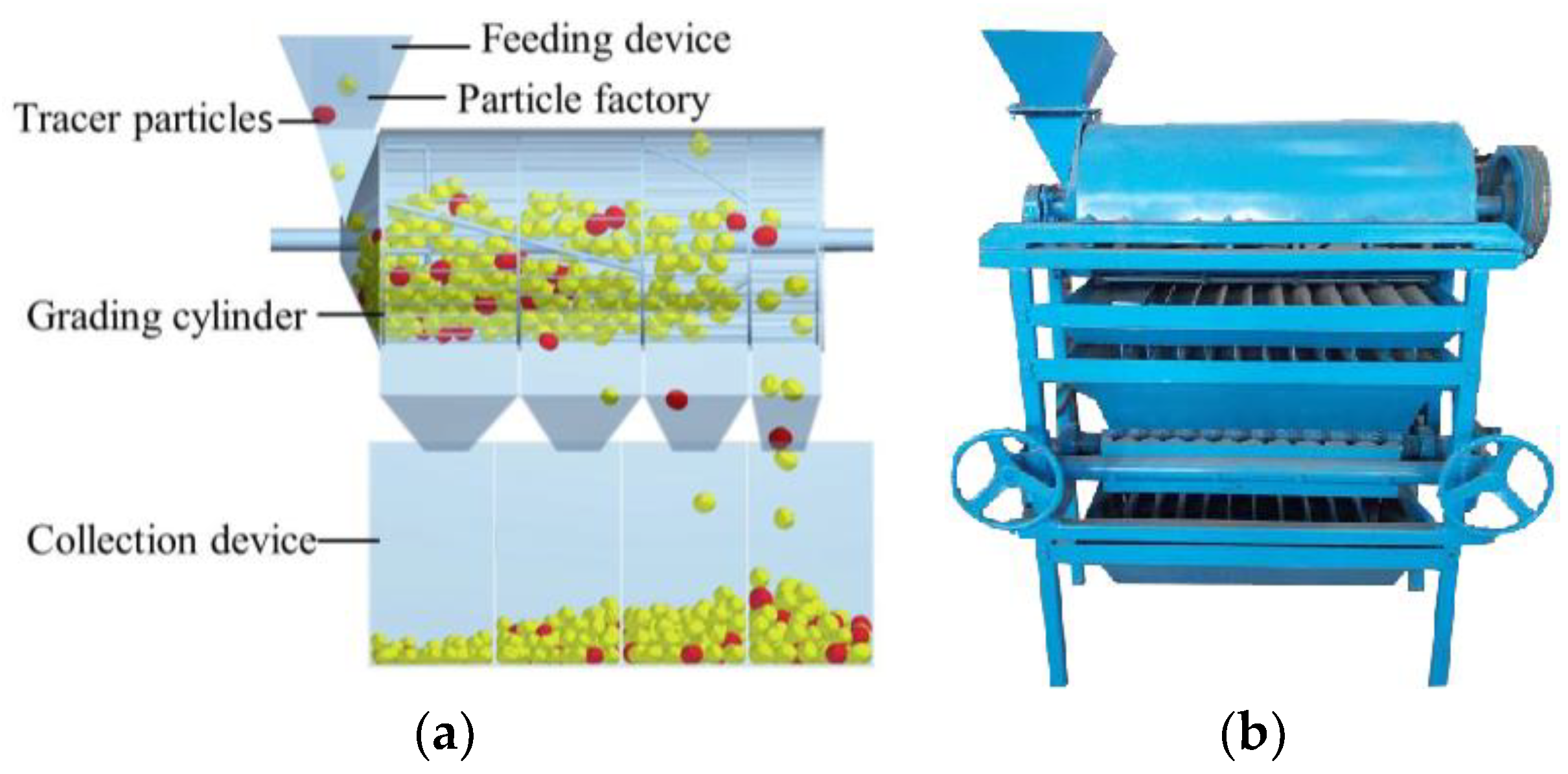
3.5.2. Verification Test of Walnut Classification

To further verify the applicability of the simulation model and its parameters, the calibration results were confirmed by the walnut classification experiment in this study. The validation methods of simulation models are divided into direct and indirect validation. The direct observation of the particle behaviour inside the classifying drum is still challenging due to the opaqueness inside the classifying drum and the complexity of the classifying environment. Therefore, indirect validation was performed in this paper using residence time, which is one of the crucial methods to measure whether the simulation is close to the actual [35,36].

Detailed experimental settings are introduced as follows: the rotation speed of the classification roller was 28 rpm (theoretical optimum rotation speed), and a particle plant was set in the hopper, which produced walnut particles conforming to the size distribution continuously and stably at the rate of 30 pcs/s. After the filling rate of the classification roller reached 30%, the stable particle stream was formed in the roller, and the walnut production rate was changed to 15 pcs/s. Meanwhile, 100 walnuts were marked randomly, and the time of random samples from entering into the hopper to leaving of classification roller was recorded (Figure 10a). Subsequently, an actual classification experiment was conducted. Before the investigation, 100 walnuts with consistent dimensions with those of random simulation samples were selected. They were dyed and used as tracking particles in the actual experiment. The frequency converter was adjusted to increase the rotation speed of the walnut classification roller to 28 rpm and adjust the walnut feeding-in rate at 30 pcs/s. After the filling rate of the classification, roller reached 30%, and the stable particle stream was formed in the roller, the walnut feeding-in rate was changed to 15 pcs/s. Dyed tracking particles were added in under the same feeding-in volume. The time taken by tracking particles from entering the hopper to leaving the classification roller was recorded by a high-speed camera (Figure 10b). The results demonstrated that the relative error of the average staying time between the simulation and the physical tests was 0.671%. Subsequently, the residence time of walnuts in the grading drum was dimensionless and processed by first dividing the residence time into equal time gradients. Each time gradient was noted as T_i. Then, the dimensionless residence time-related variables were calculated according to Equations (10)–(13). The calculation formula of dimensionless residence time is expressed as follows [37]:

$$E(t)=\frac{\mathrm{C}(t)\overline{t}}{{\displaystyle \int {}_0^{\infty }\mathrm{C}(t)d(t)}}$$

(10)

$$E(t_i)=\frac{\mathrm{C}(t_i)}{{\displaystyle \sum {}_i^{N_S}\mathrm{C}(t_i)\Delta t_i}}$$

(11)

$$E(\theta )=E(t)\overline{t}$$

(12)

$$\theta =\frac{T_{i}C\left(t_i\right)}{\overline{t}}$$

(13)

where E(t) is the distribution function; C(t_i) is the ratio of kernels to total tracer particles kernels being graded at the moment t_i, i = {1, 2, 3,..., N_S}; △t_i is the time difference between adjacent gradients, t is the mean residence time; and θ is the dimensionless residence time. Figure 11 shows the results. The distribution curves of the dimensionless staying time in the simulation and physical tests are in good agreement, but there is still a tiny difference. The reasons are analyzed as follows. Although parameter settings in the simulation and physical tests are basically consistent, they are not entirely the same. Due to the simplification of the particle model, the simulation cannot simulate vibration and thermal energy consumption, all of which can cause differences. However, the simulation test results present a consistent overall trend with physical test results. The error is controlled within the acceptable range (<5%), indicating that parameter calibration results are accurate and effective.

4. Conclusions

(1)

Intrinsic parameters of walnuts were measured via physical tests. Moisture contents in the walnut kernel and shell were 3.53% and 6.51%, respectively. Density, shear modulus, and stacking angle were reported as 527 kg/m³, 2.4 × 10⁷, and 20.12°, respectively. Measurable contact parameters included walnut–walnut collision recovery coefficient (0.14~0.46), walnut–steel plate collision recovery coefficient (0.16~0.48), and walnut–steel plate static friction coefficient (0.16~0.36). The inversion simulation test determined the values of walnut–steel plate rolling friction coefficient (0~0.2), walnut–walnut static friction coefficient (0~0.12), and walnut–walnut static friction coefficient (0.1~0.3).

(2)

The Plackett–Burman test results revealed that walnut–walnut static friction coefficient, walnut–walnut rolling friction coefficient, and walnut–steel plate static friction coefficient exerts significant effects on the stacking angle of walnuts, whereas rest contact parameters have insignificant effects. The optimal value intervals of three significant parameters are determined quickly through the steepest ascent experiment. The quadratic regression models of three crucial parameters were constructed using the Box–Behnken test. According to ANOVA, BE and C² significantly affect the stacking angle of walnuts, and B² and E² have substantial effects. The rest items can impact the stacking angle of walnuts to some extent, but such effects are not significant.

(3)

Three crucial parameters are optimized by targeting the physical stacking angle. Finally, the walnut–walnut static friction coefficient is 0.19, the walnut–walnut rolling friction coefficient is 0.11, and the walnut–steel plate static friction coefficient is 0.25. According to verification by three groups of parallel tests, the relative error is 0.068%. The simulation stacking angle is quite similar to the physical test result regarding value and morphology. Finally, the dimensionless staying time distribution diagrams between actual and simulation classifications are compared, revealing small fluctuations and consistent trends. Hence, the mechanical classification simulation of thin-skinned walnuts based on DEM modeling is feasible.

References

1. Rao, G.; Sui, J.; Zhang, J. Metabolomics reveals significant variations in metabolites and correlations regarding the maturation of walnuts (Juglans regia L.). Biol. Open 2016, 5, 829–836. [Google Scholar] [CrossRef] [PubMed] [Green Version]
2. Zhang, H.; Liu, H.L.; Zeng, Y.; Tang, Y.R.; Zhang, Z.G.; Che, J. Design and Performance Evaluation of a Multi-Point Extrusion Walnut Cracking Device. Agriculture 2022, 12, 1494. [Google Scholar] [CrossRef]
3. Liu, M.Z.; Li, C.H.; Cao, C.M.; Wang, L.Q.; Li, X.P.; Che, J.; Yang, H.M.; Zhang, X.W.; Zhao, H.Y.; He, G.Z.; et al. Walnut fruit processing equipment: Academic insights and perspectives. Food Eng. Rev. 2021, 13, 822–857. [Google Scholar] [CrossRef]
4. Shi, M.C.; Liu, M.Z.; Li, C.H.; Cao, C.M.; Li, X.Q. Design and Experiment of Cam Rocker Bidirectional Extrusion Walnut Shell Breaking Device. Trans. Chin. Soc. Agric. Mach. 2022, 53, 140–150. [Google Scholar]
5. Cao, C.M.; Luo, K.; Peng, M.L.; Wu, Z.M.; Liu, G.Z.; Li, Z. Experiment on winnowing mechanism and winnowing performance of hickory material. Trans. Chin. Soc. Agric. Mach. 2019, 50, 105–112. [Google Scholar]
6. Niu, H.; Wang, Z.T.; Tang, Y.R.; Zhang, H.; Lan, H.P.; Zhang, Y.C. Design and test of walnut classification device based on discrete element method. Trans. Chin. Jour. Agric. Mech. Resear. 2021, 43, 91–95. [Google Scholar]
7. Zhao, H.B.; Huang, Y.X.; Liu, Z.D.; Liu, W.Z.; Zheng, Z.Q. Applications of discrete element method in the research of agricultural machinery: A review. Agriculture 2021, 11, 425. [Google Scholar] [CrossRef]
8. Tan, Y.; Yu, Y.; Fottner, J.; Kessler, S. Automated measurement of the numerical angle of repose (aMAoR) of biomass particles in EDEM with a novel algorithm. Powder Technol. 2021, 388, 462–473. [Google Scholar] [CrossRef]
9. Zhou, L.; Yu, J.Q.; Liang, L.S.; Wang, Y.; Yu, Y.J.; Yan, D.X.; Sun, K.; Liang, P. DEM Parameter Calibration of Maize Seeds and the Effect of Rolling Friction. Processes 2021, 9, 914. [Google Scholar] [CrossRef]
10. Yan, D.X.; Yu, J.Q.; Wang, Y.; Zhou, L.; Tian, Y.; Zhang, N. Soil Particle Modeling and Parameter Calibration Based on Discrete Element Method. Agriculture 2022, 12, 1421. [Google Scholar] [CrossRef]
11. Xie, C.; Yang, J.W.; Wang, B.S.; Zhuo, P.; Li, C.S.; Wang, L.H. Parameter calibration for the discrete element simulation model of commercial organic fertiliser. Int. Agrophysics 2021, 35, 107–117. [Google Scholar] [CrossRef]
12. Fang, M.; Yu, Z.H.; Zhang, W.J.; Cao, J.; Liu, W.H. Friction coefficient calibration of corn stalk particle mixtures using Plackett-Burman design and response surface methodology. Powder Technol. 2022, 396, 731–742. [Google Scholar] [CrossRef]
13. Peng, C.W.; Xu, D.J.; He, X.; Tang, Y.H.; Sun, S.L. Parameter calibration of discrete element simulation model for pig manure organic fertiliser treated with Hermetia illucen. Trans. Chin. Soc. Agric. Eng. 2020, 36, 212–218. [Google Scholar]
14. Ma, Y.H.; Song, C.D.; Xuan, C.Z.; Wang, H.Y.; Yang, S.; Wu, P. Parameters calibration of discrete element model for alfalfa straw compression simulation. Trans. Chin. Soc. Agric. Eng. 2020, 36, 22–30. [Google Scholar]
15. Coetzee, C.J. Calibration of the discrete element method and the effect of particle shape. Powder Technol. 2016, 297, 50–70. [Google Scholar] [CrossRef]
16. Chen, C.; Venkitasamy, C.; Zhang, W.P.; Khir, R.; Upadhyaya, S.; Pan, Z.L. Effective moisture diffusivity and drying simulation of walnuts under hot air. Int. J. Heat Mass Transf. 2020, 150, 119283. [Google Scholar] [CrossRef]
17. González-Montellano, C.; Fuentes, J.M.; Ayuga-Téllez, E.; Ayuga, F. Determination of the mechanical properties of maise grains and olives required for use in DEM simulations. J. Food Eng. 2012, 111, 553–562. [Google Scholar] [CrossRef]
18. Zeng, Y.; Jia, F.G.; Xiao, Y.W.; Han, Y.L.; Meng, X.Y. Discrete element method modelling of impact breakage of ellipsoidal agglomerate. Powder Technol. 2019, 346, 57–69. [Google Scholar] [CrossRef]
19. ASAE S368. 4 DEC2000 (R2017); Compression Test of Food Materials of Convex Shape. American Society of Agricultural and Biological Engineers: St. Joseph, MI, USA, 2008.
20. Dietzel, A.; Raßbach, H.; Krichenbauer, R. Material testing of decorative veneers and different approaches for structural-mechanical modelling: Walnut burl wood and multilaminar wood veneer. BioResources 2016, 11, 7431–7450. [Google Scholar] [CrossRef]
21. Al-Hashemi, H.M.B.; Al-Amoudi, O.S.B. A review on the angle of repose of granular materials. Powder Technol. 2018, 330, 397–417. [Google Scholar] [CrossRef]
22. Roessler, T.; Katterfeld, A. DEM parameter calibration of cohesive bulk materials using a simple angle of repose test. Particuology 2019, 45, 105–115. [Google Scholar] [CrossRef]
23. Xia, R.; Li, B.; Wang, X.W.; Li, T.J.; Yang, Z.J. Measurement and calibration of the discrete element parameters of wet bulk coal. Measurement 2019, 142, 84–95. [Google Scholar] [CrossRef]
24. Sandeep, C.S.; Luo, L.; Senetakis, K. Effect of grain size and surface roughness on the normal coefficient of restitution of single grains. Materials 2020, 13, 814. [Google Scholar] [CrossRef] [Green Version]
25. Wei, H.; Nie, H.; Li, Y.; Saxén, H.; He, Z.J.; Yu, Y.W. Measurement and simulation validation of DEM parameters of pellet, sinter and coke particles. Powder Technol. 2020, 364, 593–603. [Google Scholar] [CrossRef]
26. Dai, Z.W.; Wu, M.L.; Fang, Z.C.; Qu, Y.B. Calibration and Verification Test of Lily Bulb Simulation Parameters Based on Discrete Element Method. Appl. Sci. 2021, 11, 10749. [Google Scholar] [CrossRef]
27. Hong, Y.L.; Jia, F.G.; Tang, Y.R.; Liu, Y.; Zhang, Q. Influence of granular coefficient of rolling friction on accumulation characteristics. Trans. Chin. Act. Phy. Sin. 2014, 63, 173–179. [Google Scholar]
28. Zhao, L.; Zhou, H.P.; Xu, L.Y.; Song, S.Y.; Zhang, C.; Yu, Q.X. Parameter calibration of coconut bran substrate simulation model based on discrete element and response surface methodology. Powder Technol. 2022, 395, 183–194. [Google Scholar] [CrossRef]
29. Coetzee, C.J. Calibration of the discrete element method. Powder Technol. 2017, 310, 104–142. [Google Scholar] [CrossRef]
30. Jiang, W.; Wang, L.H.; Tang, J.; Yin, Y.C.; Zhang, H.; Jia, T.P.; Qin, J.W.; Wang, H.Y.; Wei, Q.K. Calibration and Experimental Validation of Contact Parameters in a Discrete Element Model for Tobacco Strips. Processes 2022, 10, 998. [Google Scholar] [CrossRef]
31. Cao, X.L.; Li, Z.H.; Li, H.W.; Wang, X.C.; Ma, X. Measurement and calibration of the parameters for discrete element method modeling of rapeseed. Processes 2021, 9, 605. [Google Scholar] [CrossRef]
32. Li, Q.L. The Research of Granular Piling and Bulk Material Transfer Process Using DEM Simulation. Master’s Thesis, Northeastern University, Shenyang, China, 2010. [Google Scholar]
33. Ding, X.T.; Wei, Y.Z.; Yan, Z.Y.; Zhu, Y.T.; Cao, D.D.; Li, K.; He, Z.; Cui, Y.J. Simulation and Experiment of the Spiral Digging End-Effector for Hole Digging in Plug Tray Seedling Substrate. Agronomy 2022, 12, 779. [Google Scholar] [CrossRef]
34. Yu, S.Y.; Bu, H.R.; Dong, W.C.; Jiang, Z.; Zhang, L.X.; Xia, Y.Q. Calibration of Physical Characteristic Parameters of Granular Fungal Fertilizer Based on Discrete Element Method. Processes 2022, 10, 1564. [Google Scholar] [CrossRef]
35. Landry, H.; Thirion, F.; Lague, C.; Roberge, M. Numerical modeling of the flow of organic fertilisers in land application equipment. Comput. Electron. Agric. 2006, 51, 35–53. [Google Scholar] [CrossRef]
36. Cao, B.; Jia, F.G.; Zeng, Y.; Han, Y.L.; Meng, X.Y.; Xiao, Y.W. Effects of rotation speed and rice sieve geometry on turbulent motion of particles in a vertical rice mill. Powder Technol. 2018, 325, 429–440. [Google Scholar] [CrossRef]
37. Njeng, A.B.; Vitu, S.; Clausse, M.; Dirion, J.L.; Debacq, M. Effect of lifter shape and operating parameters on the flow of materials in a pilot rotary kiln: Part I. Experimental RTD and axial dispersion study. Powder Technol. 2015, 269, 554–565. [Google Scholar] [CrossRef]
Figure 1. Three-dimensional geometric size of walnuts.
Agriculture 13 00104 g001
Figure 2. Elastic modulus measurement test.
Agriculture 13 00104 g002
Figure 3. The stacking angle acquisition of walnuts. (a) Physical test diagram of the walnut diagram; (b) Grey processing diagram of the walnut stacking angle; (c) Profiles of the walnut stacking angle and fitting diagram.
Agriculture 13 00104 g003
Figure 4. Walnut–walnut collision recovery coefficient measurement test.
Agriculture 13 00104 g004
Figure 5. Measurement test of the walnut–steel plate static friction coefficient.
Agriculture 13 00104 g005
Figure 6. The construction process of the DEM simulation model of walnuts. (a) 3D scanning model of walnuts; (b) Mesh model of walnuts; (c) Simulation model of walnuts.
Agriculture 13 00104 g006
Figure 7. DEM simulation model of cylinder lifting.
Agriculture 13 00104 g007
Figure 8. Belt error of the inversion test.
Agriculture 13 00104 g008
Figure 9. Comparison between simulation results and physical test results of stacking angle. (a) Physical test; (b) Simulation test.
Agriculture 13 00104 g009
Figure 10. Comparison between the simulation test and physical test of walnut classification. (a) Physical test; (b) Simulation test.
Agriculture 13 00104 g010
Figure 11. Comparison of the dimensionless staying time of walnuts.
Agriculture 13 00104 g011