Abstract
Several studies have identified a host of factors to be considered when attempting to reduce food postharvest loss (PHL). However, very few studies have ranked those factors by their importance in driving PHL. This study used the Random Forest model to rank the critical drivers of PHL in maize, mango, and tomato, cultivated in Tanzania, Kenya, and Nigeria, respectively. The study then predicted the maize, mango, and tomato PHLs by changing the levels of the most critical drivers of PHL and the number of farmers at each level. The results indicate that the most critical drivers of PHL consist of pre-harvest and harvest variables in the field, such as the quantity of maize harvested in the maize value chain, the method used to know when to begin mango harvest, and the type of pest that attacks plants in the tomato value chain. Furthermore, changes in the levels of a critical driver and changes in the number of smallholder farmers at a given level both have an impact on PHL, although the impact of the former is much higher than the latter. This study also revealed that the critical drivers of PHL can be categorized as either passive and difficult to manipulate, such as the geographic area within which a smallholder farmer lives, or active and easier to control, such as services provided by the Rockefeller Foundation YieldWise Initiative. Moreover, the affiliation of smallholder farmers to the YieldWise Initiative and a smallholder farmer’s geographic location are ubiquitous critical drivers across all three value chains. Finally, an online dashboard was created to allow users to explore further the relationship between several critical drivers, the PHL of each crop, and a desired number of smallholder farmers.
1. Introduction
Maize, mango, and tomato are essential crops in Tanzania, Kenya, and Nigeria, respectively. One way to observe this importance is by comparing each crop’s annual production to all the other primary crops in each country. Maize in Tanzania, mango in Kenya, and tomato in Nigeria ranked in the 97th, 92nd, and 76th percentile of all primary crops, respectively, in 2019 [1]. Additionally, maize is cultivated by most Tanzanian farmers and occupies 45 percent of Tanzania’s cultivated land [2]. Meanwhile, mango production in Kenya, notably the Apple and Ngowe varieties, which are the most prevalent, has increased rapidly over the last decade and is expected to reach an annual production of 1.1 MT in 2022 [3]. Nigeria is the largest producer of tomatoes in Sub-Saharan Africa (SSA), and tomato is a key vegetable consumed throughout the country [4].
Besides production quantities, the nutritional facet of each crop is also valuable in understanding the importance of the crops within the respective country. For example, maize has been reported to provide about 60 percent of Tanzanian’s dietary calories and 50 percent of their proteins [5], making it an important food crop in several parts of Tanzania [6]. Mangos contain high β-carotene content, which is a precursor of vitamin A. Hence, either fresh or dried, mango fruits could reduce vitamin A deficiency in Kenya in vulnerable groups such as women and children [7]. Tomato are a rich source of lycopene, beta-carotene, folate, potassium, vitamin C, flavonoids, and vitamin E, hence, may be considered a valuable component of a cardioprotective diet [8].
Lastly, the economic importance of each crop, particularly for the benefit of smallholder farmers (SHFs), has been well reported in several studies. In Tanzania, for example, SHFs contribute over 80 percent of Tanzania’s total maize production [5], while mango farming in Kenya and tomato farming in Nigeria constitute a major income generator for many SHF households [4,9,10].
Yet, despite the evident nutritional and economic value that maize, mango, and tomato crops bring to the populations of SSA, large quantities of these crops are lost during or after harvest [11], thus never reaching the end consumer. For instance, in Tanzania, maize postharvest losses (PHL) of up to 18 percent have been reported along the entire value chain [12]. Similarly, mango and tomato production is usually accompanied by a major PHL, estimated at 40–50% [13,14]. Hence, PHL reduction efforts, especially in SSA, could be a catalyst for increasing profit for food value chain actors while at the same time boosting food availability and ultimately improving food security [5,15]. To this end, several PHL reduction initiatives have emerged over the last decade, predominantly in SSA, which remains the most food-insecure region of the world [16].
Notably, the United Nations Sustainable Development Goals (SDG12.3) aim, by 2030, to reduce food losses along production and supply chains, including postharvest losses [17]. Additionally, The Rockefeller Foundation launched the YieldWise Initiative (YWI) in 2016, which implemented several interventions to help smallholder farmers reduce their PHL in Tanzania, Kenya, and Nigeria [18]. Following the implementation of the YWI, surveys were conducted to collect farm-level data [19].
While the survey instruments used in the YWI captured many explanatory variables related to PHL, identifying critical drivers from such a large number of covariates using standard statistical methods is rather challenging [20]. Therefore, this study used a predictive modeling approach from the field of machine learning to first identify the most critical drivers of PHL from the large numbers of explanatory variables recorded in the datasets and their respective impact on PHL in the maize, mango, and tomato value chains. The advantages of using predictive modeling to this effect include, but are not limited to, their high speed in generating results [21] and their higher predictive accuracy than explanatory statistical models [22]. Moreover, predictive models are well suited for exploring and analyzing diverse data [20,23]. They can capture underlying complex patterns and relationships in the data [22] and quantify relationships between predictors and outcomes [24]. Furthermore, they are well suited for identifying important variables derived from a large dataset. Therefore, this study used the Random Forest predictive model approach to identify the most critical drivers of PHL in the maize, mango, and tomato value chains and predict their impact. Lastly, an online dashboard was created to allow users to predict maize, mango, and tomato PHLs by varying several critical drivers of a value chain and the number of farmers at once. The dashboard is described in Appendix A and can be accessed through the following link: https://phldashboard.shinyapps.io/phldashboard/ (accessed on 8 May 2023).
2. Materials and Methods
2.1. Data Summary
For each value chain, the data collected contained multiple explanatory variables, such as farm demographics, agricultural practices, storage methods, YieldWise affiliation or interventions, and PHL quantity incurred by the farmer between the harvest and point of sale. In each value chain, PHL was expressed as the quantitative and qualitative losses accumulated between harvest and point of sale [19]. After extensively cleaning the YWI survey data, the maize value chain dataset contained 22 explanatory variables and 381 observations (Table 1), the mango value chain dataset contained 21 explanatory variables and 753 observations (Table 2), and the tomato value chain dataset contained 25 explanatory variables and 503 observations (Table 3). Each observation represents a SHF who responded to the survey.

Table 1.
Maize value chain data summary.
Table 2.
Mango value chain data summary.
Table 3.
Tomato value chain data summary.
2.2. Random Forest
Predictive models range from linear models to decision trees, neural networks, support vector machines, cluster models, expert systems, etc. Each type has its strengths and weaknesses. However, the Random Forest predictive model was deemed more appropriate for this study’s objectives since it does not require any distributional assumptions [25] to analyze the complex YWI data. Furthermore, Random Forests are more effective when predictors are categorical and are not converted into dummy variables [24], as is the case in the YWI datasets. They are robust to a noisy response [24], fast to execute, require minimal storage [26], and, overall, are an effective tool in prediction [27]. Lastly, a Random Forest analysis can create several predictive models called decision trees and then combine them [21] to produce more precise predictions [22].
Random Forest models can be divided into two main categories: regression and classification. Regression Forests are used to predict a quantitative or continuous response, whereas classification Forests are used to predict a qualitative or categorical response [28]. Because the response variables in this study are maize, mango, and tomato PHL (quantitative), the regression Random Forest was used. Fundamentally, the Random Forest regression model consists of recording the predictions of each regression tree, Tb, for a new observation and then taking the average over B trees [23]:
where
prediction outcome of each regression tree b for a new observation x
total number of regression trees in the Random Forest model
sum of divided by the for a new observation x
The Random Forest predictive model was built using R software (RStudio, Boston, MA, USA). The overarching process used to attain the objectives of this study is shown in Figure 1. Further, the specific procedures used in this study are detailed within the following subsections. In addition, it should be noted that a first step in this study’s procedures was to conduct an extensive screening and cleaning process, as described by [19].
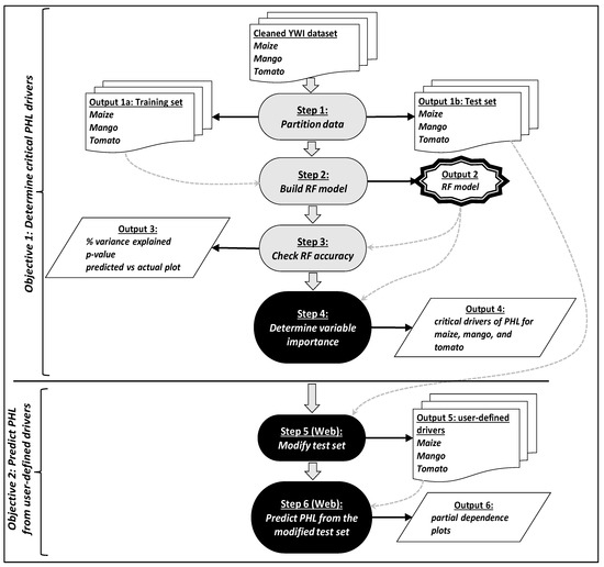
Figure 1.
Regression Random Forest model and predictions. Web refers to the online dashboard.
2.3. Random Forest
To prevent the Random Forest model from overfitting and to accurately evaluate it, it is important to split the data into a training set and a testing set [29]. The training set was used to develop the model, while the test or validation set was used to evaluate the model’s performance [24]. Several splitting rules can be used to partition data; however, empirical studies show that the best results are obtained when 20–30% of the data are used for testing and the remaining 70–80% are used for training [29]. Within this study, partitioning the maize, mango, and tomato datasets was accomplished through the DataPartition() function [30] and resulted in training sets of 269, 530, and 354 observations and test sets of 112, 223, and 149 observations in the maize, mango, and tomato value chain datasets, respectively (Figure 1 step 1).
2.4. Tuning the Random Forest Model
The Random Forest package and the Classification and Regression Training (caret) package were first loaded to simplify the tuning process. Then, three key parameters were considered to improve the model’s accuracy, namely: the random seed, the number of trees to be built in the predictive model, and the number of predictors randomly sampled at each split, also referred to as “mtry” in R.
Setting a random seed allows the results of the predictive model to be reproduced [28], since the Random Forest predictive model is built by selecting predictors randomly. The random seed was set as set.seed(1234) by using the set.seed() function [28]. The number of trees specifies how many trees will be built to populate the Random Forest. The default value is generally set at 500 [31], since a larger number of trees in a Forest only increases its computational cost, has no significant performance gain [32], and could yield overfitting [33]. Hence, the number of trees in this study was left to R’s default setting of 500 trees. As for the number of predictors randomly sampled at each split, the RandomForest() function calculates this value by dividing the total number of predictors found in the dataset by three for the regression Forest [28]. Since the maize dataset contained 22 predictors, the mango dataset, 21, and the tomato dataset, 25, the resulting mtry values were seven for the maize and mango value chain predictive models and eight for the tomato model. Three Random Forest predictive models were built for each value chain’s dataset. Each Random Forest predictive model’s significance was computed using the rfUtilities package and the rf.significance() function. In addition to the significance of the predictive models, the proportion of variance explained and predicted vs. actual plots was also generated to assess further the accuracy of each Random Forest predictive model.
2.5. Variable Importance
The variable importance calculation identifies important predictors or variables highly related to the response variable [34]. Hence, computing the variable importance was essential in achieving this study’s first objective, which consists of identifying the most critical drivers of maize, mango, and tomato PHL. The variable importance was computed along with the corresponding p-values by using the rfPermute package and the rfPermute() and rp.importance() functions. The variable importance was expressed in units of “percent increase in mean squared error (%IncMSE)”, which represents the mean decrease in accuracy in predictions when a given predictor or independent variable is excluded from the predictive model [28]. Hence, the higher the %IncMSE, the greater the importance of the corresponding variable in the predictive model. After computing the variable importance, the critical drivers of PHL were identified as those variables whose %IncMSE were significant (p-value < 0.05) (see Appendix B). Critical drivers with the highest %IncMSE were referred to as “most critical drivers”.
2.6. Predictions
Partial dependence plots were generated for each model as they are useful in interpreting the complexity of the Random Forest model [35] by displaying the relationship between the predicted outcome (PHL) and predictors of interest (critical drivers) [36]. Partial dependence plots were first generated by using the plotmo package, plotmo() function, and method = "partdep" argument [37] to have an overall view of the changes in the predicted PHL as a function of several variables contained in the dataset (Appendix C).
Additional partial dependence plots were also created to explore predicted PHL changes by varying the levels or subsets of a given critical driver. This process entailed altering a critical driver of interest in the test set while leaving all other critical drivers of PHL unchanged and subsequently running the predict() function on the modified test sets. The process of altering a critical driver of interest varied depending on whether the critical driver was categorical or numerical. When a critical driver of interest was categorical, all the levels of that critical driver were changed to a single level of interest (Figure 1 step 5), then the predict() function was run to predict PHL as a function of the changes made. The predicted PHL values were subsequently averaged over the total number of observations (Figure 1 step 6) and plotted on a bar graph, with the predicted average on the vertical axis and the chosen subset of the critical drivers on the horizontal axis. However, when the critical driver was numerical, it was first altered by adding a constant to each observation (Figure 1 step 5), then the predict() function was run to predict PHL as a function of the changes made (Figure 1 step 6). The predicted PHL values were subsequently plotted in a line graph, and placed on the vertical axis, while the altered values of the numerical driver were placed on the horizontal axis. While creating partial dependence plots helps understand the marginal effect that one or two critical drivers have on the predicted PHL, adding more than two critical drivers to the plot makes it difficult to visualize. Therefore, an online dashboard was created using the Shiny package to assess PHL by varying the subsets of one or more critical drivers and the number of farmers.
3. Results
3.1. Random Forest Models
The proportion of variance explained (R-squared) was low for the predictive models of the three value chains (Table 4). The low proportion of variance explained is also reflected in the predicted vs. actual value plots of each crop chain (Figure 2).
Table 4.
Summary of the Random Forest predictive model for each value chain.
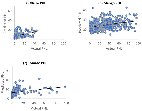
Figure 2.
Predicted PHL vs. actual PHL.
Obtaining such low R-squared values in a Random Forest regression model is not uncommon, especially when using a large dataset with irregular patterns [25], such as the YWI dataset. The fact that the PHL values were estimated by farmers and not measured likely led to errors, which in turn contributed to the lower R-squared values, as is sometimes the case in social science studies [38]. One way to minimize the errors caused by estimating would be to measure PHL by quantifying each crop’s total weight loss and subsequently expressing it as a percentage of the total harvested weight [39]. The Random Forest model summary also produced the mean squared residual values listed in Table 4, which can be used to compare alternative predictive models to the Random Forest predictive models used in this study.
3.2. Critical Drivers of PHL
Overall, the number of critical drivers of PHL in the mango and tomato value chains shown in Figure 3b and Figure 3c, respectively, is approximately three times larger than those in the maize value chain shown in Figure 3a. Hence, these results suggest that perishable crops have more critical drivers of PHL than nonperishable crops. Kiaya [40] supports this notion, as PHL in nonperishable crops is primarily due to exogenous factors such as moisture, insects, or rodents, while PHL in perishable crops is usually due to exogenous factors and endogenous factors such as respiration, transpiration, and germination.
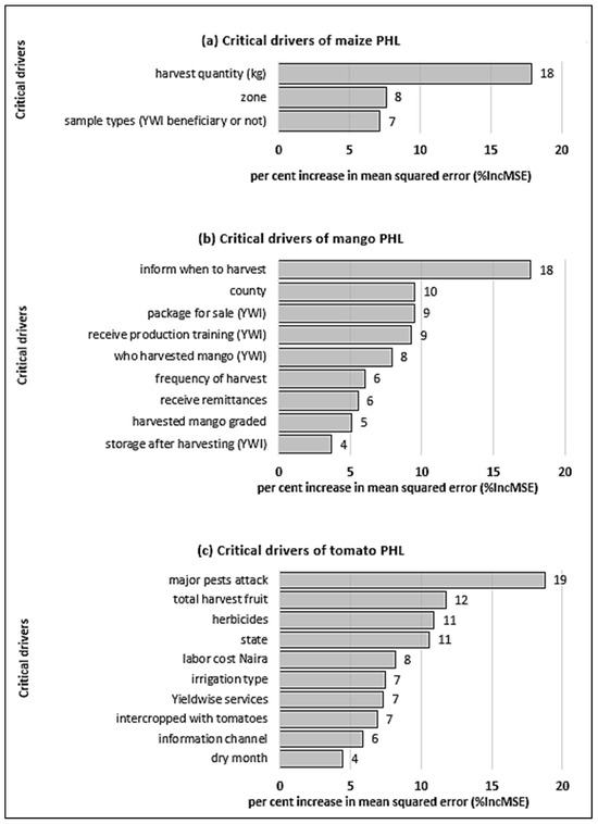
Figure 3.
Critical drivers of PHL.
Additionally, the most critical drivers of PHL, labeled “the quantity (kg) of maize harvested by a smallholder farmer” (Figure 3a), “the method used to know when to begin mango harvest” (Figure 3b), and “the type of pest that attacked the tomato plant” (Figure 3c), are all related to either pre-harvest or harvest activities. Hence, these results suggest that PHL reduction efforts should start before a harvest and continue during the harvest. Incidentally, several studies have attempted to understand how pre-harvest factors affect PHL. For example, [41] looked at how physiological processes and field management strategies influenced the ultimate quality of perishable crops. Similarly, [42] established that the prevention of pre-harvest infection of maize by toxigenic A. flavus strains should be a critical control point to reduce PHL due to aflatoxin contamination.
The per cent increase in mean squared error (%IncMSE) represents the mean decrease of accuracy in predictions when a given predictor or independent variable is excluded from the predictive model. YWI refers to critical drivers related to the YieldWise Initiative.
Lastly, two types of critical drivers were ubiquitous across all three crop value chains (Figure 3). First, the geographic location of the smallholder farmer (SHF) was labeled as “zone” in the maize value chain, “province” in the mango value chain, and “state” in the tomato value chain. Second, the affiliation of a SHF with the YWI defined as the “sample types” in the maize value chain, the “type of packaging” material in the mango value chain, and the "YWI services" in the tomato value chain. These results also indicate that the YWI played an important role as a driver of PHL reduction in the three value chains [43]. While the geographic location of a SHF can be difficult to modify [44], the various YWI services could be further explored to identify combinations that best reduce PHL. For this purpose, an online dashboard was created and made accessible at https://phldashboard.shinyapps.io/phldashboard/ (accessed on 8 May 2023). Screenshots of the dashboard can be found in Appendix A.
3.3. Assessing the Critical Drivers of PHL
The assessment of the critical drivers of PHL was carried out through partial dependence plots (Figure 4). These show the relationship between the most critical driver in each value chain, the PHL of each crop, and the number of SHFs. In the maize value chain, the results reveal that as the quantity of harvested maize increases, typically to more than 1000 kg, the maize PHL decreases, regardless of the change in the number of farmers.
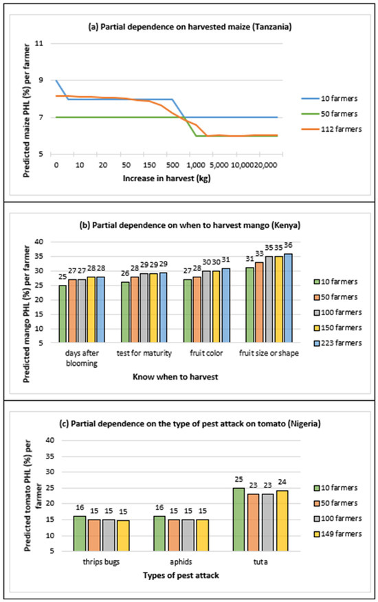
Figure 4.
Partial dependence plots for the most critical drivers of PHL.
In the mango value chain, counting the number of days after blooming to know when to begin harvest was associated with the least PHL. Incidentally, several studies have used the number of days after blooming to either determine the optimal mango harvest date to mitigate PHL during storage [45] or know when mango fruit develops the best organoleptic characteristics during ripening [46,47]. The partial dependence plot in Figure 4b also reveals that the mango PHL increases as the levels change from “days after blooming” to “fruit size or shape”. Moreover, the PHL increases monotonically as the number of farmers at each level changes from 10 to 263. However, the PHL increase due to changes in the levels (from "days after blooming" to “fruit size or shape”) is larger than the increase due to changes in the number of farmers (from 10 to 223) at each level. These results suggest that an optimum PHL mitigation practice or technology should be identified first before increasing its adoption among farmers.
In the tomato value chain, Thysanoptera, ”thrips bugs”, and Emitteri, ”aphids”, are equally associated with less PHL than the tomato leaf miner Tuta absoluta, “tuta”. Incidentally, other studies have reported the lepidoptera “tuta” as a destroyer of tomato plants in seven northern states in Nigeria, mainly due to SHFs lacking knowledge of integrated pest management practices [48,49]. Like the maize and mango value chains, as the levels of the "types of pest attack" change from Thysanoptera, “thrips bugs”, to Emitteri, “aphids”, and then to Tuta absoluta, “tuta” (Figure 4c), the shift in tomato PHL is more pronounced than when changing the number of farmers at each level.
In addition to the established relationship between the levels of various critical drivers and PHLs, it should be noted that PHL is mainly impacted by the change in the levels of a critical driver rather than the change in the number of SHFs at each level.
Since PHL is a multifaceted issue that requires considering multiple critical drivers at a time, an online dashboard was created to explore the relationship between critical drivers, the PHL of each crop, and the desired number of SHFs. The ability to insert a selected number of farmers in the dashboard allows the user to predict PHLs based on a new, arbitrary number of farmers that are not part of the YWI dataset. The online dashboard is accessible at https://phldashboard.shinyapps.io/phldashboard/ (accessed on 8 May 2023) and is described in Appendix A.
4. Conclusions
This study used Random Forest modeling to analyze the YWI data collected by the Rockefeller Foundation YieldWise Initiative in three value chains, namely maize in Tanzania, mango in Kenya, and tomato in Nigeria. The following conclusions emerged from this analysis.
- Three critical drivers of PHL were identified in the maize value chain, nine in the mango value chain, and ten in the tomato value chain. Hence, perishable crops such as tomato and mango have more critical drivers to consider when attempting to reduce PHL than nonperishable crops such as maize.
- The most critical drivers of PHL were the quantity of maize harvested by a smallholder farmer in the maize value chain, the method used to know when to begin mango harvest in the mango value chain, and the type of pest that attacked the tomato plant in the tomato value chain. It was then noted that the most critical drivers are all related to pre-harvest and harvest activities in the field. Hence, PHL reduction efforts should begin in the field before harvest and continue during harvest.
- The critical drivers of PHL fall into two categories: passive critical drivers that are difficult to manipulate, such as the geographic area within which a smallholder farmer lives, and active critical drivers that are easier to manage, such as the services provided by the YieldWise Initiative. Moreover, the geographic location of a smallholder farmer and the smallholder farmers’ affiliation with the YieldWise Initiative were both ubiquitous drivers across all three value chains.
- PHL is impacted by changes in the levels of a critical driver as well as changes in the number of smallholder farmers at each level, although the former has a much higher impact. Hence, the optimum PHL mitigation practices or technologies should be identified first before attempting to increase their adoption among smallholder farmers.
- An online dashboard was created to (a) visually display maize, mango, and tomato PHLs in bar graphs for the numerous variables found in the YieldWise Initiative dataset, (b) rank the critical drivers of maize, mango, and tomato PHL reduction, and (c) explore the relationship between several critical drivers in each value chain, the PHL of each crop, and a desired number of smallholder farmers.
While the data that led to the above conclusions were estimated by farmers and not measured, applying the Random Forest regression algorithm to assess effects across the three different agricultural commodity types is a strength of this research.
Author Contributions
Conceptualization, H.C., D.M. and S.O.; data curation, H.C.; formal analysis, H.C. and S.O.; investigation, H.C., D.M., S.O. and S.S.; methodology, H.C., D.M. and S.O.; software, H.C. and S.O.; visualization, H.C. and D.M.; roles/writing—original draft, H.C.; writing—review and editing, H.C. and D.M.; funding acquisition, D.M. and S.S.; project administration, D.M. and S.S.; resources, D.M. and S.S.; supervision, D.M., S.O. and S.S.; validation, D.M., S.O. and S.S. All authors have read and agreed to the published version of the manuscript.
Funding
Funding for this study was provided by The Rockefeller Foundation (2018 FOD 004), the Foundation for Food and Agriculture Research (DFs-18-0000000008), and the Iowa Agriculture and Home Economics Experiment Station (DD14481).
Data Availability Statement
An online interactive mango PHL dashboard was created at https://phldashboard.shinyapps.io/phldashboard/ (accessed on 8 May 2023) to support this study’s results.
Acknowledgments
The authors would like to thank The Rockefeller Foundation, the Foundation for Food and Agriculture Research, and the Iowa Agriculture and Home Economics Experiment Station for providing funding which made this research possible.
Conflicts of Interest
The funders had no role in the design of this study, analyses, or interpretation of data, in the writing of the manuscript, or in the decision to publish the results.
Appendix A. YieldWise Initiative PHL Data Dashboard
This online dashboard serves as a quantitative information management tool that
- Provides a visual display of the maize, mango, and tomato postharvest losses (PHLs) in the form of bar graphs as a function of the numerous variables found in the Rockefeller YieldWise Initiative datasets.
- Ranks the critical drivers of the maize, mango, and tomato PHLs in order of importance.
- Predicts the maize, mango, and tomato PHLs as a function of their three most critical drivers as well as the number of smallholder farmers of interest.
The dashboard can be accessed by copying the following link into a web browser: https://phldashboard.shinyapps.io/phldashboard/ (accessed on 8 May 2023). This will open the dashboard, which can be used as explained in Figure A1, Figure A2, Figure A3, Figure A4, Figure A5, Figure A6 and Figure A7 below.

Figure A1.
On the left-hand side of the screen is a menu item with the three value chains of the YieldWise Initiative.
Figure A1.
On the left-hand side of the screen is a menu item with the three value chains of the YieldWise Initiative.


Figure A2.
The user can expand a desired value chain by clicking on it. This will allow them to either visualize PHL or analyze PHL.
Figure A2.
The user can expand a desired value chain by clicking on it. This will allow them to either visualize PHL or analyze PHL.


Figure A3.
By selecting “Mango postharvest loss” as shown in the figure above, the user will access a list of variables. The user can then select a desired variable such as the “county” variable selected in the figure above as an example. The user will then automatically see a bar graph of various PHL along the value chain, categorized by counties. The number of farmers in each category of the county is also specified in the legend. Finally, the user can collapse the list of variables by clicking on “Mango postharvest loss” one more time.


Figure A4.
By clicking on “Analyze mango”, as shown in the figure above, the user can “combine factors”, which allows them to view PHL along the value chain as a function of combining multiple desired variables as opposed to looking at only one variable. Or the user could also select “drivers of mango PHL” to look at the critical drivers of mango PHL ranked in their order of importance, that is, from the most critical driver or variable to the least. Finally, under “Analyze mango”, the user can predict a PHL by selecting a given driver of PHL and a desired number of farmers.


Figure A5.
The figure illustrates an example of how the “combine mango factors” is used to visualize PHL along the value chain as a function of combining the “county” AND “labor cost” variables.
Figure A5.
The figure illustrates an example of how the “combine mango factors” is used to visualize PHL along the value chain as a function of combining the “county” AND “labor cost” variables.


Figure A6.
This figure shows the ranking of the drivers of mango PHL, i.e., “mango_factors” in the first column, followed by their relative importance (expressed in percent in mean squared error) in driving PHL, and the p-values in the third column. The critical drivers are factors with p < 0.05 (red text in column 3).


Figure A7.
This figure illustrates how to predict PHL. The user will first have to click on the “predict mango PHL” menu item circled in red. Then the user can select the desired subset or level of a given driver, as well as a desired number of farmers circled in blue. Lastly the user will be able to read the predicted PHL that will be displayed in the box circled in yellow based on the previously made selections.

The mango value chain was chosen as an example to illustrate how the dashboard works. The user can conduct the same operations in the maize and tomato value chains on the dashboard.
Appendix B. Variable Importance

Figure A8.
The vertical axis lists all explanatory variables found in each value chain dataset. The horizontal axis shows the %IncMSE, which represents the importance of each explanatory variable. The red bars represent the critical drivers of PHL or the explanatory variables with statistically significant importance (p < 0.05).

Appendix C. Partial Dependence Plots

Figure A9.
Partial dependence plots (PDP). PDPs illustrate the change in the response variables for given subsets of a critical driver of the highest importance in each value chain. The response variables are averages of the predicted PHLs and are located on the vertical axis. Each exhibit shows two 2D plots of the partial dependence and four 3D plots of the combined relationships between multiple critical drivers of PHL.

References
- FAO. FAOSTAT. 2021. Available online: https://www.fao.org/faostat/en/#data/QCL (accessed on 24 November 2021).
- Flanagan, K.; Robertson, K.; Hanson, C. Reducing Food Loss Setting a Global Action Agenda; World Resources Institute: Washington, DC, USA, 2019. [Google Scholar]
- Owuor, T.O. Guide to Export of Fresh and Processed Mango from Kenya: A Manual for Exporters: August 2015. Available online: https://www.scribd.com/document/432862956/Mango-Export-Guide-Final (accessed on 7 April 2023).
- The Rockefeller Foundation. Saving Tomatoes for the Sauce. 2021. Available online: https://www.rockefellerfoundation.org/wp-content/uploads/2021/04/YieldWise-Tomato-Overview-V4.pdf (accessed on 7 April 2023).
- Wilson, R.T.; Lewis, J. The Maize Value Chain in Tanzania. A report from the Southern Highlands Food Systems Programme 2015. Available online: https://www.fao.org/fileadmin/user_upload/ivc/PDF/SFVC/Tanzania_maize.pdf (accessed on 7 April 2023).
- Mboya, R.; Tongoona, P.; Derera, J.; Mudhara, M.; Langyintuo, A. The dietary importance of maize in Katumba ward, Rungwe district, Tanzania, and its contribution to household food security. Afr. J. Agric. Res. 2011, 6, 2617–2626. [Google Scholar]
- Muoki, P.N.; Makokha, A.O.; Onyango, C.A.; Ojijo, N.K.O. Potential contribution of mangoes to reduction of vitamin A deficiency in Kenya. Ecol. Food Nutr. 2009, 48, 482–498. [Google Scholar] [CrossRef] [PubMed]
- Willcox, J.K.; Catignani, G.L.; Lazarus, S. Tomatoes and cardiovascular health. Crit. Rev. Food Sci. Nutr. 2003, 43, 1–18. [Google Scholar] [CrossRef] [PubMed]
- Grant, W.; Kadondi, E.; Mbaka, M.; Ochieng, S. Opportunities for Financing the Mango Value Chain: A Case Study of Lower Eastern Kenya; FSD Kenya: Nairobi, Kenya, 2015; p. 52. [Google Scholar]
- Wangithi, C.M.; Muriithi, B.W.; Belmin, R. Adoption and dis-adoption of sustainable agriculture: A case of farmers’ innovations and integrated fruit fly management in kenya. Agriculture 2021, 11, 338. [Google Scholar] [CrossRef]
- Suri, T.; Udry, C. Agricultural Technology in Africa. J. Econ. Perspect. 2022, 36, 33–56. [Google Scholar] [CrossRef]
- APHLIS. APHLIS+. 2021. Available online: https://www.aphlis.net/en (accessed on 4 May 2021).
- Engineering for Change. Landscape analysis of Post-Harvest Technologies for Mango Production in East Africa. 2020. Available online: https://www.engineeringforchange.org/wp-content/uploads/2020/10/landscape_analysis_mango_postharvest_tech.pdf (accessed on 7 April 2023).
- Ugonna, C.; Jolaoso, M.; Onwualu, A. Tomato Value Chain in Nigeria: Issues, Challenges and Strategies. J. Sci. Res. Rep. 2015, 7, 501–515. [Google Scholar] [CrossRef]
- Sheahan, M.; Barrett, C.B. Food loss and waste in Sub-Saharan Africa: A critical review. Food Policy 2017, 70, 1–12. [Google Scholar] [CrossRef]
- Xie, H.; Perez, N.; Anderson, W.; Ringler, C.; You, L. Can Sub-Saharan Africa feed itself? The role of irrigation development in the region’s drylands for food security. Water Int. 2018, 43, 796–814. [Google Scholar] [CrossRef]
- Flanagan, K.; Lipinski, B.; Goodwin, L. SDG Target 12.3 on Food Loss and Waste: 2019 Progress Report. 2019, pp. 1–16. Available online: https://champions123.org/sites/default/files/2020-09/champions-12-3-2019-progress-report.pdf (accessed on 7 April 2023).
- The Rockefeller Foundation. YieldWise—The Rockefeller Foundation. 2022. Available online: https://www.rockefellerfoundation.org/initiative/yieldwise/ (accessed on 8 January 2022).
- Chikez, H.; Maier, D.; Sonka, S. Mango postharvest technologies: An observational study of the yieldwise initiative in Kenya. Agriculture 2021, 11, 623. [Google Scholar] [CrossRef]
- Best, K.B.; Gilligan, J.M.; Baroud, H.; Carrico, A.R.; Donato, K.M.; Ackerly, B.A.; Mallick, B. Random forest analysis of two household surveys can identify important predictors of migration in Bangladesh. J. Comput. Soc. Sci. 2020, 4, 77–100. [Google Scholar] [CrossRef]
- Finlay, S. Predictive Analytics, Data Mining and Big Data; Springer: Berlin/Heidelberg, Germany, 2014. [Google Scholar] [CrossRef]
- Shmueli, G. To explain or to predict? Stat. Sci. 2010, 25, 289–310. [Google Scholar] [CrossRef]
- Kern, C.; Klausch, T.; Kreuter, F. Tree-based machine learning methods for survey research. Surv. Res. Methods 2019, 13, 73–93. [Google Scholar] [PubMed]
- Kuhn, M.; Johnson, K. Applied Predictive Modeling; Springer Science Business Media: New York, NY, USA, 2013. [Google Scholar] [CrossRef]
- Hengsdijk, H.; de Boer, W.J. Post-harvest management and post-harvest losses of cereals in Ethiopia. Food Secur. 2017, 9, 945–958. [Google Scholar] [CrossRef]
- Criminisi, A.; Shotton, J. Decision Forests for Computer Vision and Medical Image Analysis; Springer Science Business Media: New York, NY, USA, 2013. [Google Scholar]
- Breiman, L. Random Forests. Mach. Learn. 2001, 45, 5–32. [Google Scholar] [CrossRef]
- James, G.; Witten, D.; Hastie, T.; Tibshirani, R. An Introduction to Statistical Learning; 8th Printing 2017; Springer: New York, NY, USA, 2013; Volume 102. [Google Scholar] [CrossRef]
- Gholamy, A.; Kreinovich, V.; Kosheleva, O. Why 70/30 or 80/20 Relation Between Training and Testing Sets: A Pedagogical Explanation. Comput. Sci. 2018, 1–6. [Google Scholar]
- Kuhn, M. Building predictive models in R using the caret package. J. Stat. Softw. 2008, 28, 1–26. [Google Scholar] [CrossRef]
- Williams, G. Data Mining with Rattle and R: The Art of Excavating Data for Knowledge Discovery; Springer: New York, NY, USA, 2011. [Google Scholar] [CrossRef]
- Perner, P. Machine Learning and Data Mining in Pattern Recognition. In Proceedings of the 7th International Conference, MLDM 2011, New York, NY, USA, 30 August–3 September 2011; Volume 2961. [Google Scholar]
- Couronné, R.; Probst, P.; Boulesteix, A.-L. Random forest versus logistic regression: A large-scale benchmark experiment. BMC Bioinform. 2018, 19, 27. [Google Scholar] [CrossRef]
- Grömping, U. Variable importance assessment in regression: Linear regression versus random forest. Am. Stat. 2009, 63, 308–319. [Google Scholar] [CrossRef]
- Friedman, J.H. Greedy function approximation: A gradient boosting machine. Ann. Stat. 2001, 29, 1189–1232. [Google Scholar] [CrossRef]
- Greenwell, B.M. pdp: An R package for constructing partial dependence plots. R J. 2017, 9, 421–436. [Google Scholar] [CrossRef]
- Milborrow, S. Plotting Regression Surfaces with Plotmo Stephen Milborrow. 2019. Available online: http://www.milbo.org/doc/plotmo-notes.pdf (accessed on 7 April 2023).
- Itaoka, K. Regression and Interpretation of Low R-squared. In Proceedings of the Social Research Network 3rd Meeting, Noosa, Australia, 12–13 April 2012. [Google Scholar]
- Hurburgh, C.R., Jr.; Bern, C.J.; Wilcke, W.F.; Anderson, M.E. Shrinkage and Corn Quality Changes in on-Farm Handling Operations. Trans. ASAE 1983, 26, 1854–1857. [Google Scholar] [CrossRef][Green Version]
- Kiaya, V. Post-Harvest Losses and Strategies to Reduce Them. 2014. Available online: https://www.actioncontrelafaim.org/wp-content/uploads/2018/01/technical_paper_phl__.pdf (accessed on 7 April 2023).
- Weston, L.A.; Barth, M.M. Preharvest factors affecting postharvest quality of vegetables. HortScience 1997, 32, 812–816. [Google Scholar] [CrossRef]
- Mahuku, G.; Nzioki, H.S.; Mutegi, C.; Kanampiu, F.; Narrod, C.; Makumbi, D. Pre-harvest management is a critical practice for minimizing aflatoxin contamination of maize. Food Control. 2019, 96, 219–226. [Google Scholar] [CrossRef]
- Sonka, S.; Lee, H.; Shah, S. The YieldWise Approach to Post-Harvest Loss Reduction: Creating Market-Driven Supply Chains to Support Sustained Technology Adoption. Agriculture 2023, 13, 910. [Google Scholar] [CrossRef]
- Delgado, L.; Schuster, M.; Torero, M. The Reality of Food Losses: A New Measurement Methodology; no. IFPRI Discussion Paper 01686; International Food Policy Research Institute: Washington, DC, USA, 2017; p. 40. [Google Scholar]
- Mathieu, L.; Jacques, J. Quality and maturation of mango fruits of cv. Cogshall in relation to harvest date and carbon supply. Aust. J. Agric. Res. 2006, 57, 419–426. [Google Scholar]
- Dick, E.; N’DaAdopo, A.; Camara, B.; Moudioh, E. Influence of maturity stage of mango at harvest on its ripening quality. Fruits 2009, 64, 13–18. [Google Scholar] [CrossRef]
- Stathers, T.; Holcroft, D.; Kitinoja, L.; Mvumi, B.M.; English, A.; Omotilewa, O.; Kocher, M.; Ault, J.; Torero, M. A scoping review of interventions for crop postharvest loss reduction in sub-Saharan Africa and South Asia. Nat. Sustain. 2020, 3, 821–835. [Google Scholar] [CrossRef]
- Borisade, O.A.; Kolawole, A.O.; Adebo, G.M.; Uwaidem, Y.I. The tomato leafminer (Tuta absoluta) (Lepidoptera: Gelechiidae) attack in Nigeria: Effect of climate change on over-sighted pest or agro-bioterrorism? J. Agric. Ext. Rural Dev. 2017, 9, 163–171. [Google Scholar] [CrossRef]
- Bala, I.; Mukhtar, M.M.; Saka, H.K.; Abdullahi, N.; Ibrahim, S.S. Determination of insecticide susceptibility of field populations of tomato leaf miner (Tuta absoluta) in northern Nigeria. Agriculture 2019, 9, 7. [Google Scholar] [CrossRef]


Disclaimer/Publisher’s Note: The statements, opinions and data contained in all publications are solely those of the individual author(s) and contributor(s) and not of MDPI and/or the editor(s). MDPI and/or the editor(s) disclaim responsibility for any injury to people or property resulting from any ideas, methods, instructions or products referred to in the content. |
© 2023 by the authors. Licensee MDPI, Basel, Switzerland. This article is an open access article distributed under the terms and conditions of the Creative Commons Attribution (CC BY) license (https://creativecommons.org/licenses/by/4.0/).