The Rapid Detection of Trash Content in Seed Cotton Using Near-Infrared Spectroscopy Combined with Characteristic Wavelength Selection

Abstract

Herein, we propose a new method based on Fourier-transform near-infrared spectroscopy (FT-NIR) for detecting impurities in seed cotton. Based on the spectral data of 152 seed cotton samples, we screened the characteristic wavelengths in full-band spectral data with regard to potential correlation with the trash content of seed cotton. Then, we applied joint synergy interval partial least squares (siPLS) and combinatory algorithms with the competitive adaptive reweighted sampling method (CARS) and the successive projection algorithm (SPA). In addition, we used the sparrow search algorithm (SSA), gray wolf algorithm (GWO), and eagle algorithm (BES) to optimize parameters for support vector machine (SVM) analysis. Finally, the feature wavelengths optimized via the six feature wavelength extraction algorithms were modeled and analyzed via partial least squares (PLS), SSA-SVM, GWO-SVM, and BES-SVM, respectively. The correlation coefficients, R_c and R_p, of the calibration and prediction sets were subsequently used as model evaluation indices; comparative analysis highlighted that the preferred option was the inverse estimation model as this could accurately predict the trash content of seed cotton. Subsequently, we found that the accuracy of predicting the content of impurities in seed cotton when applying the optimized SVM model of SSA combined with the feature wavelengths screened via siPLS-SPA was optimal. Thus, the optimal modeling method for inverse impurity content was siPLS-SPA-SSA-SVM, with an R_c value of 0.9841 and an R_p value of 0.9765. The rapid application development (RPD) value was 6.7224; this is >3, indicating excellent predictive ability. The spectral inversion model for determining the impurity rate of mechanized harvested seed cotton samples established herein can, therefore, determine the impurity rate in a highly accurate manner, thus providing a reference for the subsequent construction of a portable spectral detector of impurity rate. This will help objectively and quantitatively characterize the impurity rate of mechanized harvested seed cotton and provide a new tool for rapidly detecting impurities in mechanized harvested wheat. Our findings are limited by the small sample size and the fact that the model developed for estimating the impurity content of seed cotton was specific to a local experimental field and certain varieties of cotton.

1. Introduction

China is the foremost global producer of unprocessed cotton, with Xinjiang emerging as its primary hub for cultivating premium-grade cotton since the turn of the millennium. In 2022, the production of cotton in the Xinjiang region amounted to 5.391 million tons, thus representing a significant share of 90% of cotton production by the entire nation. According to the National Bureau of Statistics of China, the total area allocated for cotton cultivation in Xinjiang amounted to 2496.9 thousand hectares [1]. In the same year, this region possessed 6300 cotton-picking machines, thus resulting in an impressive mechanized harvesting rate of over 80% for cotton crops. The mechanization level in Xinjiang cotton agriculture, including planting and harvesting, has been reported to be 94.49%. At present, the region of Xinjiang has several established industrial bases for modern agricultural machinery and equipment; the central hubs for this industry are located in Urumqi, Shihezi, Korla, and Aksu [2]. The lack of established online monitoring systems restricts the real-time assessment of trash content in cotton harvested using machinery. This leads to inconsistent quality in mechanized cotton harvesting, thus impacting cotton fiber quality and severely limiting the application and promotion of mechanized cotton harvesting.

The application of image detection methods often detects cotton impurities. For example, Wang et al. [3] and others used machine vision to identify foreign fibers in cotton; Zhou et al. [4] detected foreign impurities in lint cotton using an alternating white light/fluorescence imaging detection method; Wan et al. [5] detected the trash content of seed cotton using a color wo-sided imaging method; and Zhang et al. [6,7] used a color shape method and genetic algorithm to optimize a parameter model for support vector machine (SVM) analysis to identify impurities in machine-picked cotton images. In another study, Wang et al. [8] used a local binary pattern and a grayscale covariance matrix to classify and identify impurities in seed cotton. Zhao et al. [9] used an improved ant colony algorithm to select the features of exotic fibers in cotton to classify and identify impurities, while Mustafic et al. [10] developed an imaging device with blue and UV excitation sources for the classification and identification of foreign matter in cotton.

Near-infrared (NIR) spectroscopy has attracted considerable attention over recent years because it is rapid, simple, non-destructive, and simultaneously measures multiple components [11]. Previously, researchers used various spectroscopic techniques to perform quantitative analysis. For instance, Wu et al. [12] employed near-infrared and Raman spectroscopy to develop a quantitative model for assessing mung bean moisture, protein, and total starch content. Teye et al. [13] used near-infrared spectroscopy for the non-destructive determination of total fat content in cocoa bean samples. Wang et al. [14] employed characteristic wavelength-selective near-infrared spectroscopy to rapidly detect protein content in rice. Li et al. [15] developed a generalized multi-location model based on near-infrared spectroscopy to determine the content of soluble solids in Fuji apples. Fortier et al. [16] successfully identified cotton impurities by extracting NIR spectral features from a spectral database. Azadnia et al. [17] adopted wavelength selection and machine learning techniques to rapidly detect nitrogen, phosphorus, and potassium content in apple leaves. Jiang et al. [18] designed a hyperspectral imaging system based on push-broom technology to efficiently detect and classify foreign matter on the surface of cotton lint. Chen et al. [19,20] developed a hyperspectral inversion model to determine the content of impurities in wheat and soybean. In addition, researchers have utilized classical feature wavelength selection algorithms, such as synergy interval partial least squares (siPLS) [20] and competitive adaptive reweighted sampling (CARS) [21], for the detection of impurities in cotton.

Many studies have shown that more accurate calibration models may be achieved by selecting the important spectral variables instead of using the full spectrum [22,23,24,25,26,27]. Several variable selection methods exist, such as competitive adaptive reweighted sampling (CARS), the genetic algorithm (GA), the successive projections algorithm (SPA), and the synergy interval partial least squares (siPLS) [28]. Additionally, variable selection attempts to reduce the complexity and thus improve the robustness of a calibration model [29]. Different spectral variable selection methods showed differences in terms of accuracy and parsimony. Variable selection is often highly dependent on the dataset, which seriously complicates the interpretation. The success of spectral variable selection is usually evaluated empirically via statistics of the resulting multivariate model (e.g., the cross-validated root-mean-squared error (RMSE)).

Machine vision monitoring is limited by complex algorithms and poor real-time performance. Another issue is that the content of impurities in seed cotton is much larger than that of lint cotton; in particular, seed cotton has a large number of stems, hulls, and leaves from the cotton plant that are interspersed with cotton fibers in seed cotton harvested using a cotton-picker. Fourier-transform near-infrared (FT-NIR) spectroscopy is the method of choice for the non-destructive monitoring of impurity content in seed cotton. In this study, we used long-wave Fourier-transform near-infrared spectroscopy (FT-NIR) to analyze the seed cotton harvested using cotton pickers and screened the characteristic wavelengths sensitive to trash content in seed cotton (predominantly stems, hulls, and leaves from the cotton plant). Next, the spectra of the characteristic wavelengths were used to construct an inversion model for plant trash content in seed cotton, and the detection accuracy of this method was compared with a range of other models. Our aim was to develop an alternative means of detecting traditional trash in seed cotton and provide a reference for rapidly detecting trash content in cotton.

2. Materials and Methods

2.1. Seed Cotton Samples

The test samples were obtained from the Xinjiang Iron Construction Heavy Industry test base. Samples were harvested on 15 September 2022 using a 4MZD-6 cotton-picking baler. A total of 152 samples were collected as experimental samples. The samples were placed in a sealed bag after collection; these bags were numbered and returned to the laboratory. The 152 samples were randomly divided into a calibration set of 114 samples and a prediction set of 38 samples for modeling analysis (in a 3:1 ratio).

2.2. Spectral Preprocessing

There are several spectral preprocessing methods, including multiplicative scatter correction (MSC), first derivative (FD), and second derivative (SD) with Savitzky–Golay (SG) smoothing [19]. Continuous wavelet transform (CWT) has recently been reported for spectral preprocessing. The CWT exhibits better performance than common preprocessing methods [30]. In this study, CWT was used for seed cotton spectra.

2.3. Determination of Trash Content

The percentage of impurities in seed cotton refers to the proportion (in %) of impurities contained in seed cotton. The separation of impurities is mainly performed manually [31]. The trash content was then determined by Equation (1).

$$\mathrm{Z}=\frac{{\mathrm{m}}_{\mathrm{s}}}{{\mathrm{m}}_{\mathrm{c}}}\times 100$$

(1)

In Equation (1), Z denotes the trash content (%); m_s denotes the mass of the test sample grams (g); and m_c denotes the trash content of the test sample (g).

2.4. Acquisition of FT-NIR Spectra

NIR spectra were acquired using a Fourier-transform near-infrared spectrometer (Antaris II, Thermo Fisher Scientific Corporation, Waltham, MA, USA) equipped with an indium gallium arsenide (InGaAs) detector and controlled via Resulte software (version 4, Thermo Fisher Scientific Corporation, USA). The seed cotton sample was placed into a sample cup and shaken evenly. Then, we performed an integrating sphere spectrum scan on a FT-NIR spectrometer. The spectral scanning wavenumber range was 3800–12,000 cm⁻¹. Each sample was loaded three times, with a spectral resolution of 16 cm^−1, and scanned 96 times after each loading. Scanning provides information relating to a given sample and facilitates the accurate and stable analysis of impurities. The background was scanned hourly. We collected spectra from seed cotton in absorbance mode, and the procedure was repeated three times for each sample of seed cotton to obtain their average spectra. All spectra were recorded as absorbance values.

2.5. Spectral Variable Selection

The raw spectral data featured both intrinsic information about the sample as well as extraneous information that has the potential to impact the precision of the model. The raw spectra featured a large number of redundant and uninformative variables. In addition, the informative variables also exhibited serious collinearity. The selection of spectral bands showing high correlations with the impurity content of seed cotton allowed for the improved interpretation of modeled relationships and variables. From an optimization point of view, wavelength selection could be viewed as an optimization process to maximize the predictive performance of the calibration model [32].

2.5.1. siPLS Methodology

The synergy interval partial least squares (SiPLS) algorithm is a feature band selection method and was developed based on interval partial least squares (iPLS) [33]. The whole spectral region can be divided into several equal-width subintervals via the iPLS algorithm. Then, a regression model was established for each interval using the PLS method, and the optimal number of principal factors was determined using the cross-validation method. Finally, the root-mean-square of cross-validation was considered as the accuracy measurement of the local model; the sub-interval refers to when the local model with high accuracy was taken as the feature interval. SiPLS is based on iPLS and combines the sub-intervals of several local models with higher accuracy in the same division as a whole to build a larger model; from this, the combination interval with the smallest RMSECV value was selected as the optimal feature sub-interval. SiPLS algorithms are often used in conjunction with cross-validation methods, such as syst123 cross-validation. This method evaluates the model’s predictive performance and provides an estimate of its stability and generalization ability. In this study, the interval of SiPLS was set to 14.

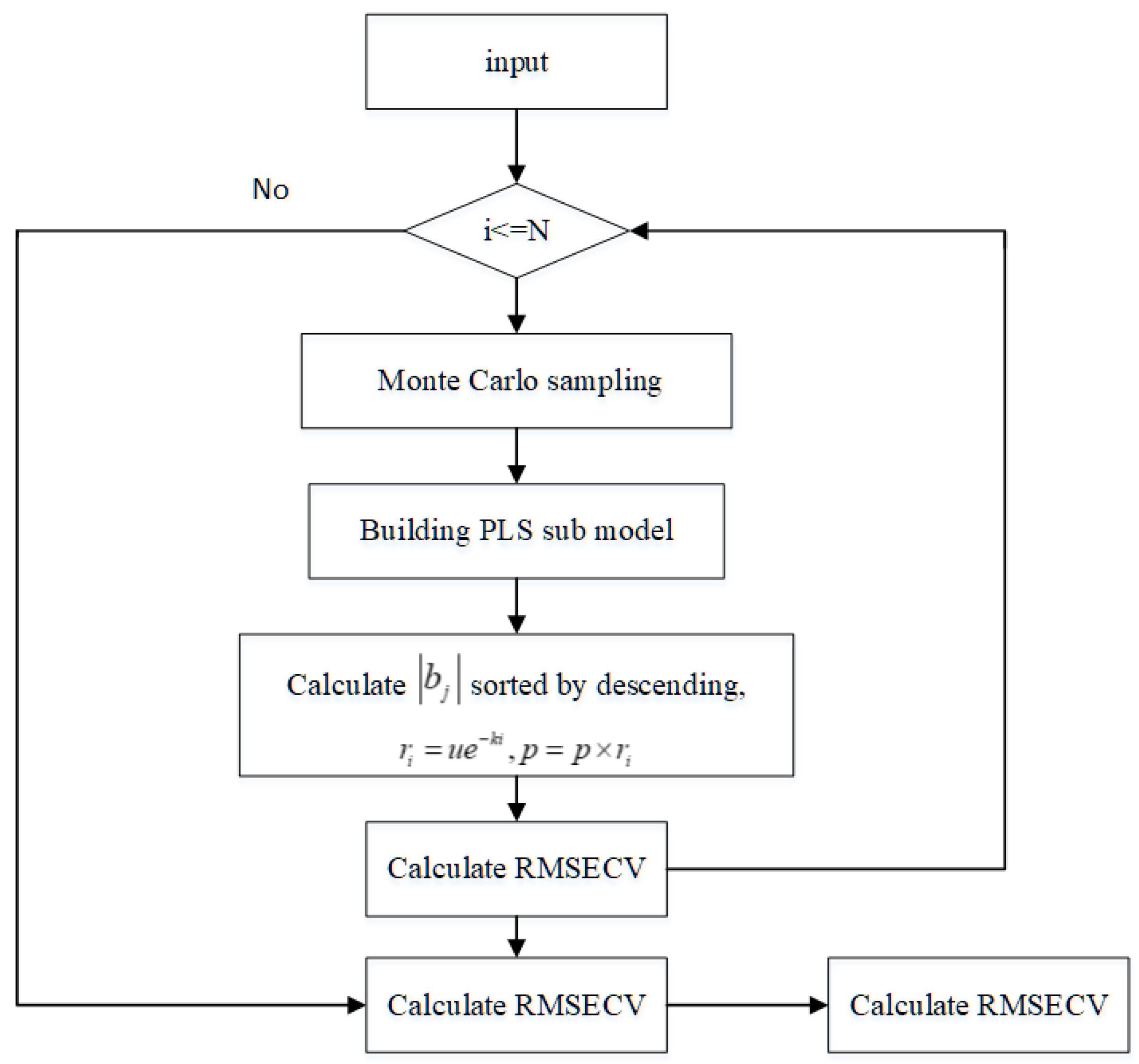
2.5.2. The CARS Algorithm

The competitive adaptive reweighted sampling (CARS) algorithm was first introduced by Li et al. [34]. To select the effective wavelength, we used CARS to select a subset of N variables via m Monte Carlo (MC) sampling runs iteratively. Finally, we selected the subset with the smallest cross-validated root-mean-square error (RMSECV) value as the optimal subset. In each sampling run, the steps can be described as follows: (a) Monte Carlo model sampling; (b) forced wavelength selection based on the exponentially decreasing function (EDF); (c) competitive wavelength selection using adaptive reweighted sampling; and (d) evaluation of the subset using cross-validation. CARS employs a simple but effective “survival of the fittest” principle and a certain degree of cross-validation. CARS adopts a simple but effective “survival of the fittest” principle and allows the selection of the optimal wavelength subset, at least to some extent. CARS can eliminate non-informative variables and perform wavelength selection to build high-performance calibration models. Incorrect parameter selection may lead to the degradation of algorithm performance or unsatisfactory feature selection results. Therefore, careful parameter tuning is required [35].

2.5.3. The SPA Algorithm

The successive projections algorithm (SPA) is a forward variable selection algorithm commonly used for multivariate calibration. The operational mechanism involves executing basic projection operations within a vector space to derive a subset of variables that exhibit minimal covariance [36]. The forward selection approach categorizes SPA since it begins by selecting a single wavelength and then computes the projections of this wavelength onto additional wavelengths in each cycle [37]. The effective wavelength can then be determined by selecting the wavelength with the highest projection value. The SPA method aims to identify wavelengths that possess minimal redundancy in their spectrum information. This selection process facilitates the identification of the most informative and important variables for subsequent analysis. The SPA algorithm can select fewer variables and significantly reduce covariance information. This algorithm is not very effective when used alone; therefore, it is usually combined with other wavelength selection algorithms.

2.6. Modeling Methods

2.6.1. PLS-Based Regression

PLS is a well-established technique in multivariate linear analysis [38]. Spectral data analysis is a commonly employed technique [19]. Here, we used partial least squares (PLS) regression analysis to develop a prediction model for quantitative outcomes using near-infrared data from seed cotton. The spectral variables were used as input data for PLS analysis and represented the X variables. Conversely, various trash contents were used as output data representing the Y variables.

The PLS method was used for analysis because this tool is able to accommodate data matrices with a greater number of variables than individuals (921 wavelengths and 260 samples). In addition, this method can analyze the covariance between the explanatory matrix, X, and the response matrix, Y, as well as identify the component of the subspace that coincides most closely with the two data matrices [38,39]. Equation (2) was used to calculate the expected value Y_p for a given sample.

$${\mathrm{Y}}_{\mathrm{p}}=\mathrm{TX}+\mathrm{b}$$

(2)

In Equation (2), T is the matrix of regression coefficients, and b is the model offset. The number of latent variables (lv) is an important parameter in developing PLS models.

2.6.2. SVM-Based Regression

A support vector machine (SVM) is a widely used classification and regression algorithm that minimizes the empirical risk and confidence interval by controlling different ratios between the empirical risk and confidence interval values, thus improving the overall generalization ability of the model [40]. This algorithm has numerous advantages; for example, it has a small generalization error, can be interpreted easily, and can solve non-linear and high-dimensional problems [41]. In this study, we mapped the linearly inseparable low-dimensional feature data to the high-dimensional space. Then, we identified the optimal hyperplane using the kernel function to minimize the distance between the samples and the hyperplane, thus establishing a linear regression model.

The kernel function is the key to the SVM algorithm. Commonly used kernel functions include the polynomial kernel function, linear kernel function, Gaussian kernel function, and radial basis function (RBF). Because the RBF kernel function can handle both linear and non-linear information in spectral data and is less susceptible to the interference of sample outliers [42], the RBF kernel function was chosen to build the SVM model. The RBF can be described as follows:

$$\mathrm{K}(x,x_k)=\exp (-\parallel x-x_k{\parallel }^2/2{\sigma }^2)$$

(3)

In Equation (3), $\parallel x-x_k\parallel$ is the distance between the input vector and the threshold vector and $\sigma$ is the broadband parameter.

Choosing the appropriate regularization parameter c and kernel function g is crucial for the performance of RBF-SVM models, although there is no accepted best method for parameter optimization for SVM machines. Intelligent optimization algorithms, such as bald eagle search (BES), sparrow search algorithm (SSA), and gray wolf optimization (GWO), have been widely used for parameter optimization for support vector machines applying spectral data; this strategy has achieved satisfactory results.

In the present study, we used SSA to optimize the parameters c and g within the SVM model. SSA is an intelligent optimization technique first introduced by Jiankai Xue in 2020 [43]. This algorithm was inspired by the foraging and antipredator actions exhibited by sparrows. The algorithm has various advantages over other methods, such as uniqueness, rapid convergence, and robust global search capabilities. In SSA, sparrows were categorized into two forms: seekers and participants, and the foraging process of sparrows was regarded as a finder and follower model with superimposed detection and warning mechanisms [44]. The finder provides the foraging area and direction for the whole sparrow population, while the follower obtains food by locating the finder. Moreover, a certain proportion of individuals in the sparrow population were selected for scouting and early warning activities. The number of optimization parameters was 2; the upper limit of optimization parameters was 100 and the lower limit was 0.01; the number of sparrows was set to 10; and the maximum number of iterations was set to 100.

The BES was first reported in 2019 [45] and represents an optimization algorithm inspired by the hunting strategies and intelligent social behaviors of bald eagles when seeking fish. In the original paper, BES hunting was divided into three phases. In the first phase (selecting a space), the bald eagle selected the space with the highest number of prey. In the second phase (searching through the space), the eagle moved through the selected space in search of prey. In the third phase (swooping), the eagle swung from the best position determined in the second phase and identified the best hunting spot. The dive started from the optimal point, and all other movements were directed to this point. The optimization results confirmed that the BES algorithm competed well with advanced metaheuristics and traditional methods. The number of optimization parameters was 2; the upper limit of optimization parameters was 100 and the lower limit was 0.01; the number of populations was set to 5; and the maximum number of iterations was set to 60.

The GWO algorithm [46] mimics the leadership hierarchy and hunting mechanisms of wild gray wolves. Four species of gray wolves (alpha, beta, delta, and omega) were used to model the leadership hierarchy. In addition, three main phases of hunting were executed to perform optimization (searching, aggression, and attacking prey). The number of optimization parameters was 2; the upper limit of optimization parameters was 100 and the lower limit was 0.01; the number of wolves was set to 10; and the maximum number of iterations was set to 50.

2.7. Model Evaluation

In the present study, the dataset was randomly divided into validation and test sets for data processing and model establishment. The validation set featured 75% of the data, while the test set featured 25%. This process was repeated five times, each employing a different random data partition into validation and test sets. This method, known as cross-validation, ensured the robustness and reliability of the model’s performance evaluation.

This method of arbitrarily separating data into training and testing sets and performing multiple validations is frequently employed in machine learning experiments to obtain more accurate and representative model evaluation outcomes. Three performance metrics were used in the present study to evaluate the experimental results: the root-mean-square error (RMSE), the coefficient of determination (R²), and rapid application development (RPD). R² measures the extent to which the independent variable explains the variance of the dependent variable. The closer the R² value is to 1, the greater the model’s ability to explain the relationship between variables and predict outcomes when data change [36]. The RMSE represents the difference between the model’s predicted and actual values; a smaller RMSE indicates a greater predictive accuracy [46]. Our objective was to minimize the RMSE to increase the model’s accuracy when predicting the target variable. The accuracies of the calibration models were categorized following the suggestions of Saeys et al. [25]. According to these established guidelines, RPD values > 3 indicate excellent predictions, while RPD values between 2.5 and 3.0 indicate good predictions. An RPD value between 2.0 and 2.5 indicates an approximate quantitative prediction, while an RPD value between 1.0 and 1.4 indicates that the model is not suitable for accurate quantitative prediction and can only differentiate between high and low values of physicochemical properties. RPD values < 1.5 indicate unsuccessful predictions.

The equations for calculating RMSE, R², and RPD are presented as Equations (4)–(6), respectively. Evaluating these measures was essential in determining the precision and predictive capacity of the constructed models.

$$\mathrm{RMSE}=\sqrt{\frac{1}{n}{{\displaystyle \sum _{i=1}^n(y_i-{\widehat{y}}_i)}}^2}$$

(4)

$${\mathrm{R}}^2=1-\frac{{\displaystyle \sum _{i=1}^n{({\widehat{y}}_i-y_i)}^2}}{{\displaystyle \sum _{i=1}^n{({\overline{y}}_{}-y_i)}^2}}$$

(5)

$$\mathrm{RPD}=\frac{\sqrt{\frac{1}{n-1}{\displaystyle \sum _{i=1}^n{(y_i-y)}^2}}}{\mathrm{RMSE}}$$

(6)

In these equations, $y_i$ indicates the predicted value of trash content in samples of seed cotton, %; ${\widehat{y}}_i$ indicates the measured value of trash content in samples of seed cotton, %; $\overline{y}$ indicates the average value of trash content in samples of seed cotton, %; and n indicates the number of samples.

2.8. Software

The development of predictive models for trash content in seed cotton was conducted with MATLAB R2021a, a software platform offered by MathWorks Inc., Natick, MA, USA. Two distinct regression techniques were utilized for modeling: SVM regression and PLS regression. Using the MATLAB R2021a software, two regression techniques were employed to develop prediction models for the trash content in seed cotton. These models enabled the estimation of trash content by utilizing spectral data obtained from samples of seed cotton. We used a range of functions, including plsregress, svmtrain, fmincon, getobjvalue, initialization, BES, GWO, and SSA.

3. Results and Discussion

3.1. Selection of Characteristic Spectral Wavelengths

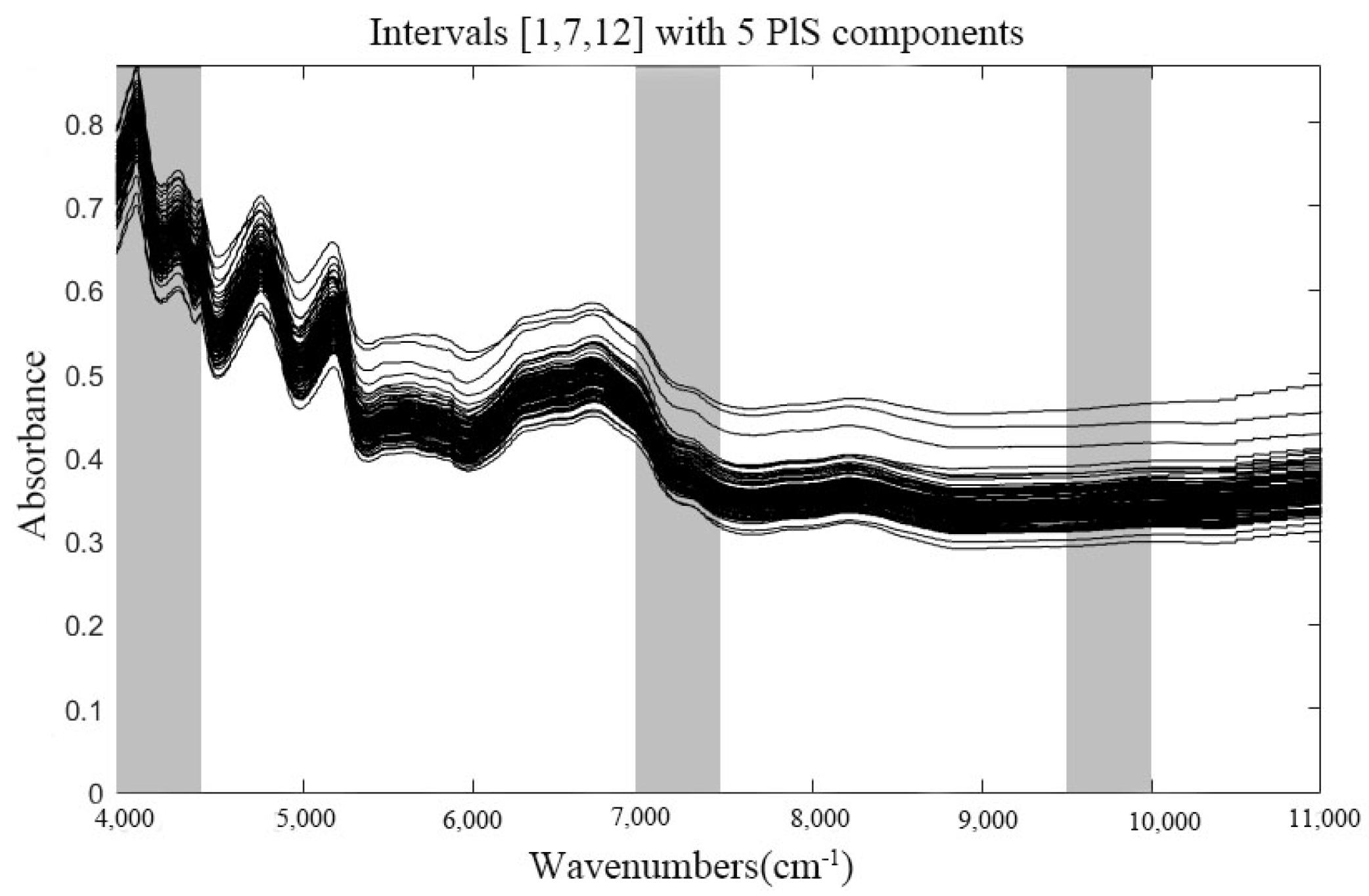
3.1.1. siPLS-Based Feature Interval Selection

The spectral information of full-band spectra contains some spectral information that is not related to seed cotton content, which will affect not only the accuracy of the model but also the calculation speed. Therefore, we used the siPLS method to divide the full-band spectra into different joint subintervals. Then, the interval with the best correlation was selected for data dimensionality reduction. The results of subinterval optimization are shown in

Table 1. Results derived from the smooth-1der Si-PLS model for selecting different spectral regions.

PLS Components	Selected Intervals	RMSECV (%)
5	[1,7,12]	0.3981
5	[1,7,9]	0.3989
5	[1,7,14]	0.3995
5	[1,7,13]	0.4001
5	[1,8,13]	0.4007
5	[1,7,11]	0.4008
4	[1,8,9]	0.4020
4	[1,11,12]	0.4022
4	[1,9,10]	0.4022
4	[1,12,13]	0.4023

. In Table 1, PLS components denote the number of principal components extracted from the input variables using the PLS algorithm; selected intervals denote the final variable intervals or ranges selected during the siPLS process. siPLS selects the most relevant variables based on assessing the importance of the variables as a subset of the final variables. RMSECV is the root-mean-square error calculated during the cross-validation. The percentage representation of the root-mean-square error, a measure of the difference between the actual observations and the cross-validated predictions, was calculated during the process. Lower values of RMSECV (%) indicate better predictive performances of the model.

The optimal subinterval selected for the final run was [1,7,12], and the minimum RMSECV value was 0.3981, resulting in a total of 197 spectral variables, accounting for 21.4% of the total variables. Next, the preferred subintervals were downscaled using the characteristic wavelength extraction algorithm to reduce the dimensionality of the data further. The application of the extraction algorithm for data dimensionality reduction further improved the accuracy of the model and simplified it. Figure 1 demonstrate RMSECV as a function of the number of PLS components for the selected intervals. Figure 2 demonstrate the optimal result of the characteristic band. The rectangle in the figure shows the preferred band.

3.1.2. The CARS Algorithm

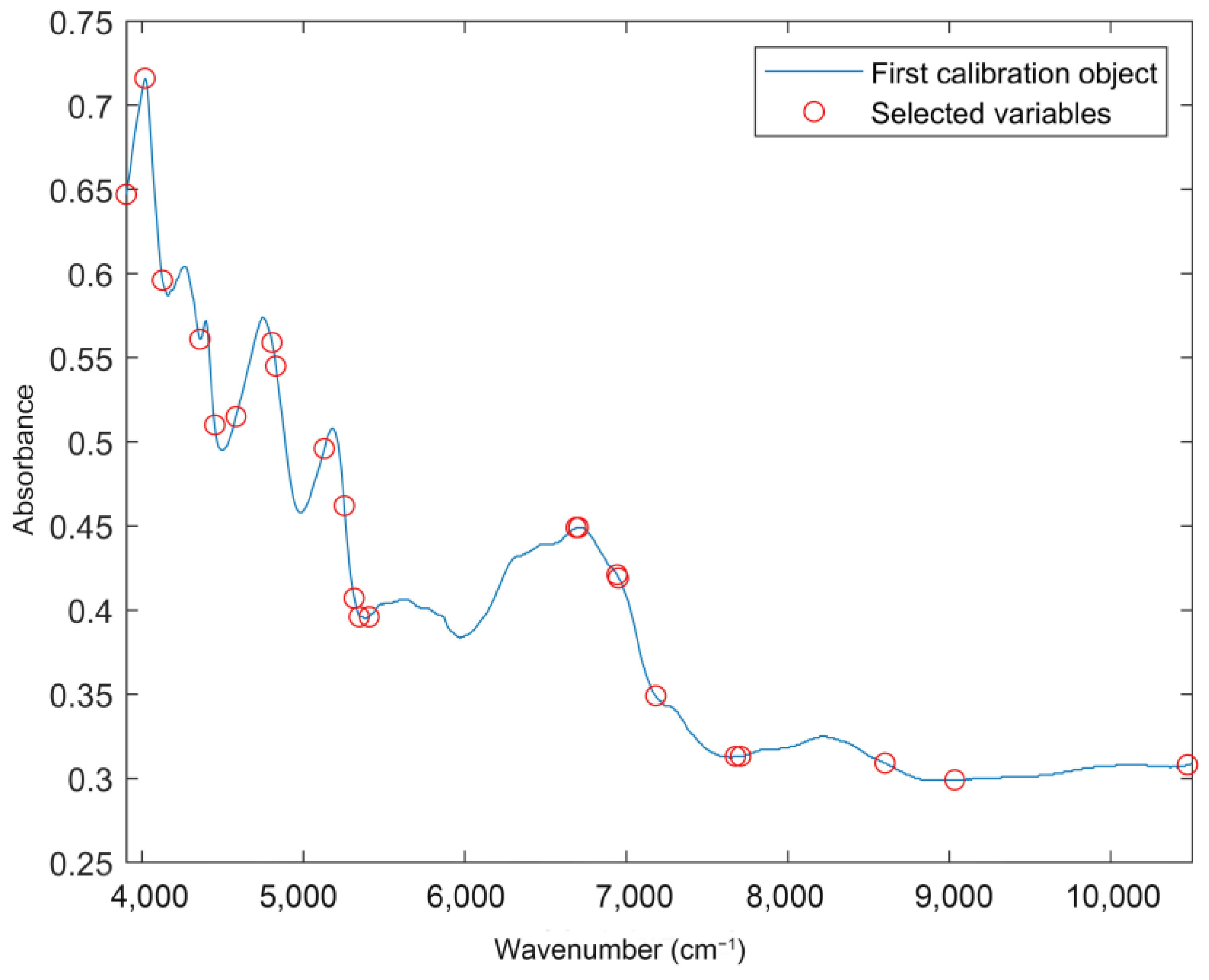
The CARS algorithm was used to select characteristic wavelengths from the 197 spectral variables previously identified using the siPLS technique. To assure the algorithm’s robustness and reliability, the number of Monte Carlo samples for CARS cross-validation was set to 200. Each sampling was random and resulted in unique outcomes for each execution of the CARS algorithm. The optimal number of feature wavelengths was determined by performing multiple validation comparisons. The integration of siPLS and CARS refined the set of characteristic wavelengths, reduced the dimensionality of the data, and improved the performance and precision of the inversion model for predicting trash content in seed cotton. The iterative nature of the CARS algorithm assured exhaustiveness in the selection process and captured the most significant spectral characteristics associated with the trash content of seed cotton.

Figure 3 is a flowchart illustrating the key steps and procedures of the CARS algorithm. The objective of the CARS algorithm was to select the most informative and pertinent wavelengths from the provided spectral data. As depicted in Figure 4, the optimally selected characteristic wavelength variables indicate which wavelengths provide the most helpful information for predicting the trash content of seed cotton. Following the application of the CARS algorithm, the number of variables selected via CARS was reduced to 55, while the number of variables selected via siPLS-CARS was reduced to 23.

Figure 4 shows the changing trend of the number of sampled variables (plot a), RMSECV values (plot b), and the regression coefficient path of each variable (plot c) with the increasing of sampling runs from one CARS running. In Figure 4a, the number of sampled variables decreases fast in the first step and then very slowly in the second step. In Figure 4b, the RMSECV values first descend from sampling runs 1–25, which indicates that the uninformative variables were eliminated. Finally, it increased rapidly due to some informative variables being removed. In Figure 4c, the lowest RMSECV was achieved, where the line was marked by an asterisk (in the 39th sampling run), when the sampling runs were increased.

3.1.3. SPA

Next, we used the successive projections algorithm (SPA) to further reduce the dimensionality of the spectral data by selecting the feature wavelengths for three distinct sets of spectral variables: the initial spectra, the 273 spectral variables identified via siPLS, and the spectral variables identified via CARS. The SPA algorithm successfully discovered 48 specific wavelengths from the original spectra that were highly pertinent for accurately predicting the impurity rate of seed cotton. The set of 273 feature variables selected via the siPLS method was further subjected to the SPA algorithm, resulting in the selection of 30 feature wavelengths. Thus, the SPA algorithm discovered nine feature wavelengths for the spectral variables specified via CARS.

The wavelengths identified played a crucial role in determining the overall prediction performance of the inversion model. Figure 5 shows the spectral variables chosen for spectral principal component analysis (SPA). The utilization of siPLS, CARS, and SPA algorithms throughout the data reduction procedure guaranteed the preservation of the most informative wavelengths while simultaneously reducing the dimensionality of the data. This led to the development of a prediction model that was more efficient in terms of its performance.

3.2. PLS-Based Regression

Table 2. PLS regression results using different wavelength selection methods.

Feature Selection	Number of Wavelengths	Modeling Methods	Calibration Set		Prediction Set		RPD
			${\mathit{R}}_{\mathit{c}}^2$	RMSEC	${\mathit{R}}_{\mathit{p}}^2$	RMSEP
siPLS	273	PLS	0.9702	0.3717	0.9273	0.5896	3.4702
CARS	55		0.9716	0.3279	0.9643	0.5389	3.0634
SPA	48		0.9700	0.3706	0.9438	0.4824	3.5236
siPLS-CARS	30		0.9687	0.3773	0.9534	0.4748	4.0613
siPLS-SPA	23		0.9753	0.3289	0.9607	0.4086	3.8976
CARS-SPA	9		0.9688	0.3514	0.9698	0.4506	3.7128

shows the outcomes of applying the generalized PLS model in conjunction with various wavelength selection techniques for determining the trash content of seed cotton. The analysis demonstrated that all models attained a prediction accuracy of 90%, thus confirming that the developed model was highly suitable for predicting trash content in seed cotton. In the PLS model, siPlS-SPA yielded better results (R2: p = 0.9607; RMSE: p = 0.4086; RPD = 3.8976). CARS yielded the worst results (R2: p = 0.9643; RMSE: p = 0.5389; RPD = 3.0643). Cross-validation was used for each model. The various parameters of each model were within normal limits and were not overfitted.

3.3. SVM- Based Regression

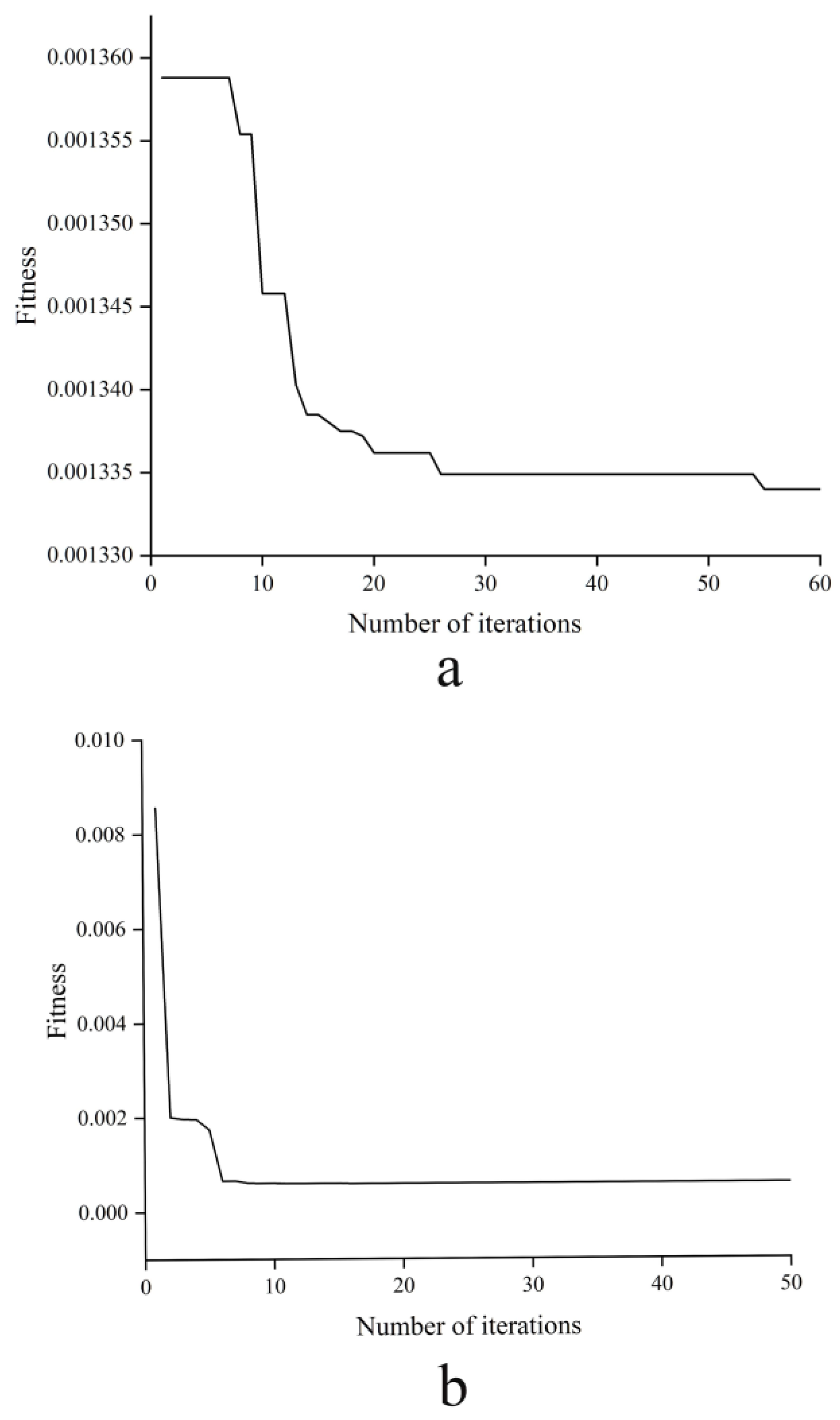
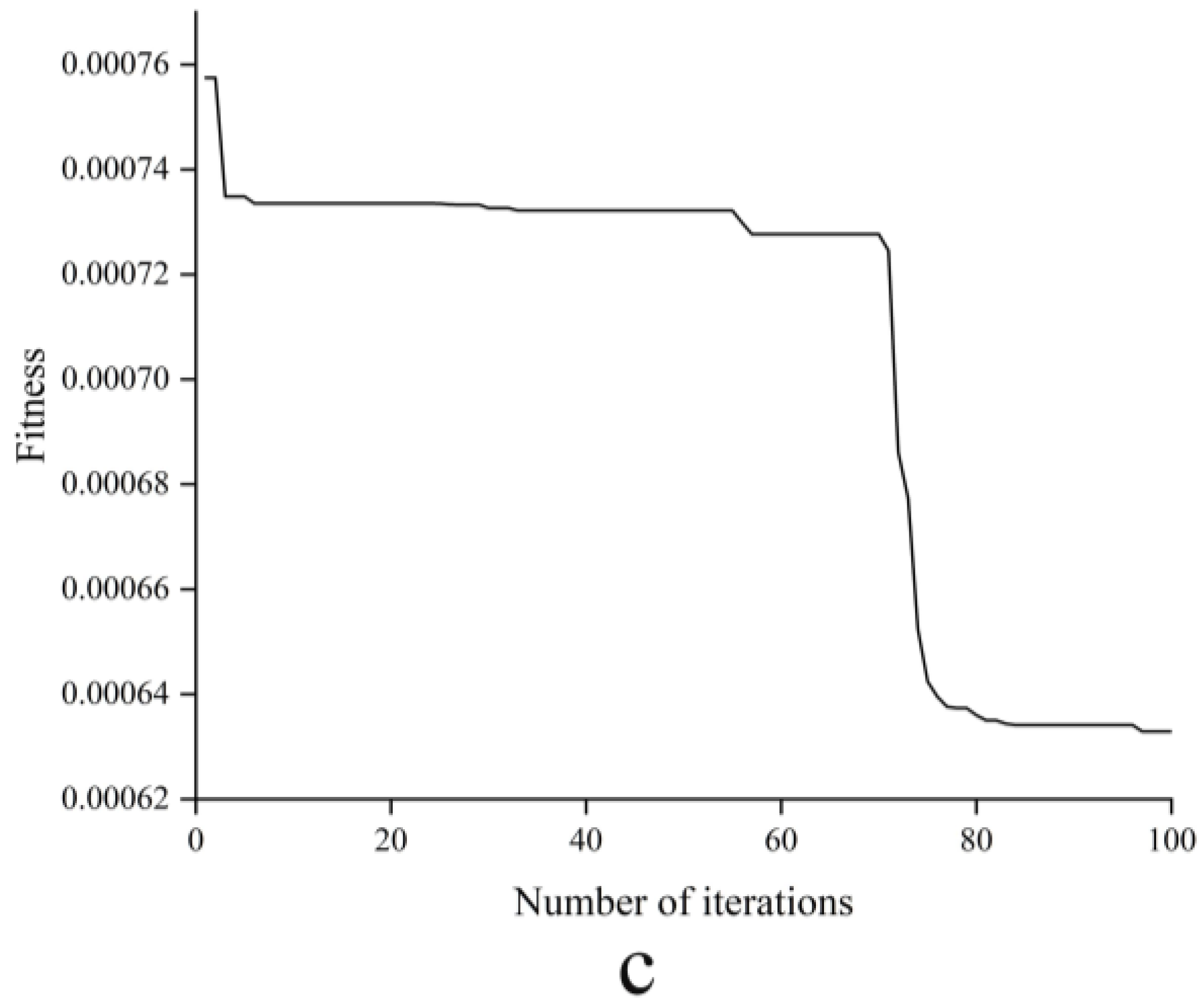
3.3.1. Optimization of SVM Based on GWO, SSA, and BES

The modeling procedure commenced by first choosing the characteristic wavelengths of the spectra. Following this, parameter configurations were established for the bald eagle search (BES), grey wolf optimizer (GWO), and sparrow search algorithm (SSA). In the BES, the parameter specifying the number of populations was assigned a value of 5, while the parameter determining the number of iterations was set to 60. The minimum value for the regularization parameter C and the kernel parameter gamma was 0.01, while the maximum was 100. The grey wolf optimizer (GWO) and the social spider algorithm (SSA) utilized comparable parameter configurations.

Figure 6 provides depictions of the optimization process. As the number of iterations grew, the fitness value of the fitness function fell, thus suggesting a reduction of the discrepancy between the final predicted value of the model and the actual value. Of the three methods under consideration, it was evident that the SSA algorithm exhibited superior optimization performance as it attained the lowest value on the vertical axis. Using parameter optimization techniques such as BES, GWO, and SSA played a significant role in identifying optimal parameters for the SVM model. Figure 6 shows that BES reached stability around 56 iterations with an adaptation of 0.001334, GWO reached stability around 21 iterations with an adaptation of 0.00015, and SSA reached stability around 97 iterations with an adaptation of 0.00063. The smaller the adaptation, the better the parameter was selected with 56, 21 and 97 iterations, respectively.

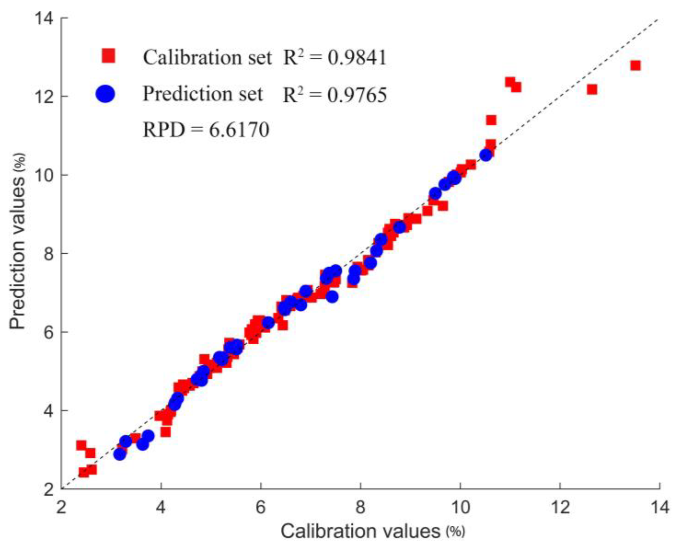
3.3.2. Modeling of Seed Cotton Impurity Prediction

In this study, we utilized six wavelength selection methods. The GWO-SVM, SSA-SVM, and BES-SVM modeling analysis incorporated specific wavelengths as independent variables. The variable that was measured and analyzed as the outcome in the final model was the amount of trash in a sample of seed cotton. The modeling results are presented in

Table 3. Performance comparison of the support vector machine (SVM) models based on different optimization algorithms.

Feature Selection	Modeling Methods	Calibration Set		Prediction Set		RPD
		${\mathit{R}}_{\mathit{c}}^2$	RMSEC	${\mathit{R}}_{\mathit{p}}^2$	RMSEP
siPLS	GWO-SVM	0.9967	0.1228	0.9274	0.5893	3.7621
CARS		0.9813	0.3034	0.8979	0.6134	3.1724
SPA		0.9947	0.1545	0.9198	0.6190	3.5785
siPLS-CARS		0.9973	0.1075	0.9294	0.6234	3.8161
siPLS-SPA		0.9910	0.2002	0.9544	0.4737	4.7506
CARS-SPA		0.9692	0.3747	0.9433	0.5240	4.2558
siPLS	SSA-SVM	0.9971	0.1147	0.9287	0.5832	3.7973
CARS		0.9883	0.2414	0.9447	0.5453	4.3125
SPA		0.9916	0.1927	0.9087	0.6621	3.3541
siPLS-CARS		0.9968	0.1188	0.9437	0.5467	4.2717
siPLS-SPA		0.9841	0.2814	0.9772	0.3355	6.7224
CARS-SPA		0.9964	0.1267	0.9551	0.4836	4.7844
siPLS	BES-SVM	0.9980	0.0949	0.9216	0.6134	3.6212
CARS		0.9880	0.2315	0.9194	0.5911	3.5710
SPA		0.9948	0.1412	0.9412	0.5392	4.1824
siPLS-CARS		0.9847	0.2620	0.9708	0.3803	5.9303
siPLS-SPA		0.9869	0.2422	0.9765	0.2900	6.6170
CARS-SPA		0.9674	0.3831	0.9785	0.2949	5.7914

, which illustrates the efficacy of each of the constructed prediction models utilizing distinct wavelength selection techniques. The models utilizing feature wavelength variables selected via the siPLS feature interval method resulted in poorer accuracies when compared to the three algorithms combined (siPLS-SPA, siPLS-CARS, and CARS-SPA). This disparity can be mainly attributed to the siPLS algorithm’s tendency to save a substantial quantity of data in the chosen feature wavelengths, encompassing certain wavelength variables that did not pertain to the trash content of seed cotton. Consequently, the accuracy of the model’s predictions was compromised, and the complexity of the model was increased due to the excessive inclusion of wavelength variables.

In contrast, combining the siPLS-SPA, siPLS-CARS, and CARS-SPA algorithms efficiently streamlined the prediction models while improving their predictive capacities. Utilizing these integrated algorithms effectively filtered out wavelength factors that exhibited a strong link with the presence of waste in seed cotton, thus enhancing the precision of predictive outcomes. In general, utilizing these integrated algorithms is highly advantageous in effectively forecasting and monitoring the level of seed cotton trash in mechanized processes.

The analysis in Table 3 demonstrates that the optimized SVM models exhibited superior prediction accuracy compared to the PLS model. The observed enhancement in the predictive performance of the models may be ascribed to the optimization of support vector machine (SVM) parameters through the utilization of GWO, SSA, and BES.

Table 3 shows that the prediction accuracy of all SVM models was lower than that of SSA-SVM, thus indicating that optimizing the parameters of SVM using the SSA algorithm improved the prediction accuracy of the model, and this effect was better than the other two optimization algorithms. The optimal prediction model was siPLS-SPA-SSA-SVM with a prediction set correlation coefficient of 0.9772; compared with the GWO-SVM and BES-SVM models, the model’s accuracy was improved by 0.0228 and 0.0007, respectively. Only 23 input variables were included in the model; therefore, this model improved both its accuracy and simplicity. Thus, the siPLS-SPA-SSA-SVM model is better than the other two optimization algorithms. The SSA-SVM model yields better predictive effects than the other two models, probably because it has the highest number of iterations and the best optimization results. However, this model was also the slowest. Therefore, we recommend selecting the SSA-SVM model when a higher prediction accuracy is needed. If faster monitoring is required, we recommend utilizing the BES-SVM model. The correlation between the predicted and calibrated values, utilizing the support vector machines (SVM) near-infrared (NIR) technique, is visually depicted in Figure 7.

3.3.3. Suggestions for Further Research

Our research provides a new strategy to monitor the impurity content of cotton; this can be performed non-destructively in a short period. If a portable spectrometer can be fitted on the cotton picker, this might provide the operator with real-time information on the impurity content of the cotton to adjust the parameters of the picker. However, some large impurities and their concentrations will affect the monitoring of impurity content; therefore, other technologies could be incorporated to gain further improvement, for example, the incorporation of images.

4. Conclusions

This study aimed to use near-infrared spectroscopy to predict the trash content of seed cotton. Our analysis involved the use of seed cotton obtained via cotton pickers and employed machine learning methods, including PLS, BES-SVM, GWO-SVM, and SSA-SVM, to establish a predictive model for the association between near-infrared (NIR) spectra of seed cotton samples and indices of trash content. A comparative analysis was also conducted to assess the model’s efficacy in predicting the trash content of seed cotton. Analysis of the prediction metrics used to construct the models (R2, RMSE, and RPD) revealed that all modeling techniques successfully predicted the trash content of seed cotton. When applying the SVM modeling technique, our findings demonstrated superior performance compared to the partial least squares (PLS) modeling technique. The SSA-SVM model exhibited superior predictive accuracy compared to the PLSR model, as evidenced by its higher R2 and lower RMSE values. This implied that the SSA-SVM modeling approach is more suited for estimating the trash content of seed cotton as it demonstrates a higher capacity to handle both linear and non-linear connections. The combination of NIR spectroscopy with SSA-SVM modeling holds significant promise for developing a quick and non-destructive method for detecting the trash content of seed cotton during harvesting. Furthermore, it is essential to note that the seed cotton utilized in our prediction set originated from a single sample batch. To ensure the robustness and reliability of this model in real-world scenarios, we recommend that future research utilize many independent prediction sets to evaluate performance fully. Integrating this efficient and expeditious near-infrared (NIR) technique with assessing the quality and traceability of seed cotton is anticipated to influence the regulation of seed cotton quality significantly.

References

1. National Bureau of Statistics of the People’s Republic of China. NSO Announcement on Cotton Production in 2022[EB/OL]. Available online: http://www.stats.gov.cn/sj/zxfb/202302/t20230203_1901689.html (accessed on 26 December 2022).
2. Central People’s Government. Xinjiang’s Cotton Mechanized Harvesting Rate Exceeds 80 Percent [EB/OL]. Available online: https://www.gov.cn/xinwen/2022-06/22/content_5697041.htm (accessed on 22 June 2022).
3. Wang, X.; Li, D.; Yang, W.; Li, Z. Lint Cotton Pseudo-foreign Fiber Detection Based on Visible Spectrum Computer Vision. Trans. Chin. Soc. Agric. Mach. 2015, 46, 7–14. [Google Scholar]
4. Zhou, F.; Ding, T.; Qu, X. Detection of foreign materials in lint cotton with a white-light/fluorescence alternating imaging method. J. Tsinghua University. Sci. Technol. 2010, 50, 1234–1238. [Google Scholar]
5. Wan, L.; Pang, Y.; Zhang, R.; Jiang, Y.; Zhang, M.; Song, F.; Chang, J.; Xia, B. Rapid measurement system for the impurity rate of machine-picked seed cotton in acquisition. Trans. Chin. Soc. Agric. Eng. 2021, 37, 182–189. [Google Scholar]
6. Zhang, C.; Li, L.; Dong, Q.; Ge, R. Recognition for machine picking seed cotton impurities based on GA-SVM model. Trans. Chin. Soc. Agric. Eng. 2016, 32, 189–196. [Google Scholar]
7. Zhang, C.; Li, L.; Dong, Q.; Ge, R. Recognition Method for Machine-harvested Cotton Impurities Based on Color and Shape Features. Trans. Chin. Soc. Agric. Mach. 2016, 47, 28–34. [Google Scholar]
8. Wang, H.; Li, H. Classification recognition of impurities in seed cotton based on local binary pattern and gray level co-occurrence matrix. Trans. Chin. Soc. Agric. Eng. 2015, 31, 236–241. [Google Scholar]
9. Zhao, X.; Li, D.; Yang, B.; Ma, C.; Zhu, Y.; Chen, H. Feature selection based on improved ant colony optimization for online detection of foreign fiber in cotton. Appl. Soft Comput. 2014, 24, 585–596. [Google Scholar] [CrossRef]
10. Mustafic, A.; Li, C.Y.; Haidekker, M. Blue and UV LED-induced fluorescence in cotton foreign matter. J. Biol. Eng. 2014, 8, 29. [Google Scholar] [CrossRef]
11. Wang, Z.; Liu, J.; Zeng, C.; Bao, C.; Li, Z.; Zhang, D.; Zhen, F. Rapid detection of protein content in rice based on Raman and near-infrared spectroscopy fusion strategy combined with characteristic wavelength selection. Infrared Phys. Technol. 2023, 129, 104563. [Google Scholar] [CrossRef]
12. Li, J.; Zhang, Y.; Zhang, Q.; Duan, D.; Chen, L. Establishment of a multi-position general model for evaluation of watercore and soluble solid content in ‘Fuji’ apples using online full-transmittance visible and near infrared spectroscopy. J. Food Compos. Anal. 2023, 117, 105150. [Google Scholar] [CrossRef]
13. Fortier, C.A.; Rodgers, J.E.; Cintron, M.S.; Cui, X.; Foulk, J.A. Identification of cotton and cotton trash components by Fourier-transform near-infrared spectroscopy. Text. Res. J. 2010, 81, 230–238. [Google Scholar] [CrossRef]
14. Azadnia, R.; Rajabipour, A.; Jamshidi, B.; Omid, M. New approach for rapid estimation of leaf nitrogen, phosphorus, and potassium contents in apple-trees using Vis/NIR spectroscopy based on wavelength selection coupled with machine learning. Comput. Electron. Agric. 2023, 207, 107746. [Google Scholar] [CrossRef]
15. Wang, K.; Jiang, Y.; Li, C. Detection and Discrimination of Cotton Foreign Matter Using Push-Broom Based Hyperspectral Imaging: System Design and Capability. PLoS ONE 2015, 10, e0121969. [Google Scholar]
16. Chen, M.; Ni, Y.; Jin, C.; Xu, J.; Yuan, W. High spectral inversion of wheat impurities rate for grain combine harvester. Trans. Chin. Soc. Agric. Eng. 2019, 35, 22–29. [Google Scholar]
17. Chen, M.; Xu, J.; Jin, C.; Zhang, G.; Ni, Y. Inversion model of soybean impurity rate based on hyperspectral. J. China Agric. Univ. 2019, 24, 160–167. [Google Scholar]
18. Wu, M.; Li, Y.; Yuan, Y.; Li, S.; Song, X.; Yin, J. Comparison of NIR and Raman spectra combined with chemometrics for the classification and quantification of mung beans (Vigna radiata L.) of different origins. Food Control 2023, 145, 109498. [Google Scholar] [CrossRef]
19. Teye, E.; Huang, X. Novel Prediction of Total Fat Content in Cocoa Beans by FT-NIR Spectroscopy Based on Effective Spectral Selection Multivariate Regression. Food Anal. Methods 2015, 8, 945–953. [Google Scholar] [CrossRef]
20. Li, Y.; Yang, X. Quantitative analysis of near infrared spectroscopic data based on dual-band transformation and competitive adaptive reweighted sampling. Spectrochim. Acta Part A Mol. Biomol. Spectrosc. 2023, 285, 121924. [Google Scholar] [CrossRef]
21. Li, Q.; Huang, Y.; Song, X.; Zhang, J.; Min, S. Moving window smoothing on the ensemble of competitive adaptive reweighted sampling algorithm[J]. Spectrochim. Acta Part A Mol. Biomol. Spectrosc. 2019, 214, 129–138. [Google Scholar]
22. Xu, S.; Zhao, Y.; Wang, M.; Shi, X. Determination of rice root density from Vis–NIR spectroscopy by support vector machine regression and spectral variable selection techniques. Catena 2017, 157, 12–23. [Google Scholar] [CrossRef]
23. Sarathjith, M.C.; Das, B.S.; Wani, S.P.; Sahrawat, K.L. Variable indicators for optimum wavelength selection in diffuse reflectance spectroscopy of soils. Geoderma 2016, 267, 1–9. [Google Scholar] [CrossRef]
24. Vohland, M.; Ludwig, M.; Thiele-Bruhn, S.; Ludwig, B. Determination of soil properties with visible to near- and mid-infrared spectroscopy: Effects of spectral variable selection. Geoderma 2014, 223–225, 88–96. [Google Scholar] [CrossRef]
25. Li, H.; Liang, Y.; Xu, Q.; Cao, D. Key wavelengths screening using competitive adaptive reweighted sampling method for multivariate calibration. Anal. Chim. Acta 2009, 648, 77–84. [Google Scholar] [CrossRef] [PubMed]
26. Bian, X.; Wang, K.; Tan, E.; Diwu, P.; Zhang, F.; Guo, Y. A selective ensemble preprocessing strategy for near-infrared spectral quantitative analysis of complex samples. Chemom. Intell. Lab. Syst. 2020, 197, 103916. [Google Scholar] [CrossRef]
27. Jiang, H.; Liu, L.; Chen, Q. Rapid determination of acidity index of peanuts by near-infrared spectroscopy technology: Comparing the performance of different near-infrared spectral models. Infrared Phys. Technol. 2022, 125, 104308. [Google Scholar] [CrossRef]
28. Miao, X.; Miao, Y.; Gong, H.; Tao, S.; Chen, Z.; Wang, J.; Chen, Y.; Chen, Y. NIR spectroscopy coupled with chemometric algorithms for the prediction of cadmium content in rice samples. Spectrochim. Acta Part A Mol. Biomol. Spectrosc. 2021, 257, 119700. [Google Scholar] [CrossRef] [PubMed]
29. Zou, X.; Zhao, J.; Povey, M.J.W.; Holmes, M.; Mao, H. Variables selection methods in near-infrared spectroscopy. Anal. Chim. Acta 2010, 667, 14–32. [Google Scholar]
30. Ma, C.; Shao, X. Continuous Wavelet Transform Applied to Removing the Fluctuating Background in Near-Infrared Spectra. J. Chem. Inf. Comput. Sci. 2004, 44, 907–911. [Google Scholar] [CrossRef]
31. GB/T 21397-2002; Cotton Harvesters: Certification and Accreditation Administration. Standardization Administration of the People’s Republic of China: Beijing, China, 2008.
32. Wang, L.S.; Wang, R.J. Determination of soil pH from Vis-NIR spectroscopy by extreme learning machine and variable selection: A case study in lime concretion black soil. Spectrochim. Acta Part A Mol. Biomol. Spectrosc. 2022, 283, 121707. [Google Scholar] [CrossRef]
33. Kumar, K. Competitive adaptive reweighted sampling assisted partial least square analysis of excitation-emission matrix fluorescence spectroscopic data sets of certain polycyclic aromatic hydrocarbons. Spectrochem. Acta Part A Mol. Biomol. Spectrosc. 2021, 244, 118874. [Google Scholar] [CrossRef]
34. Yang, G.; Li, Y.; Zhen, F.; Xu, Y.; Liu, J.; Li, N.; Sun, Y.; Luo, L.; Wang, M.; Zhang, L. Biochemical methane potential prediction for mixed feedstocks of straw and manure in anaerobic co-digestion. Bioresour. Technol. 2021, 326, 124745. [Google Scholar] [CrossRef] [PubMed]
35. Wold, S.; Sjöström, M.; Eriksson, L. PLS-regression: A basic tool of chemometrics. Chemom. Intell. Lab. Syst. 2001, 58, 109–130. [Google Scholar] [CrossRef]
36. Araújo, M.C.U.; Saldanha, T.C.B.; Galvao, R.K.H.; Yoneyama, T.; Chame, H.C.; Visani, V. The successive projections algorithm for variable selection in spectroscopic multicomponent analysis. Chemom. Intell. Lab. Syst. 2001, 57, 65–73. [Google Scholar] [CrossRef]
37. Yuan, Q.; Wang, Q.D.; Liu, S.; Wu, K. A systematic Chandra study of Sgr A⋆: II. X-ray flare statistics. Mon. Not. R. Astron. Soc. 2018, 473, 306–316. [Google Scholar] [CrossRef]
38. Geladi, P.; Kowalski, B.R. Partial least-squares regression: A tutorial. Anal. Chim. Acta 1986, 185, 1–17. [Google Scholar] [CrossRef]
39. Jiang, H.; Yuan, W.; Ru, Y.; Chen, Q.; Wang, J.; Zhou, H. Feasibility of identifying the authenticity of fresh and cooked mutton kebabs using visible and near-infrared hyperspectral imaging. Spectrochem. Acta Part A Mol. Biomol. Spectrosc. 2022, 282, 121689. [Google Scholar] [CrossRef] [PubMed]
40. Chen, Q.; Zhao, J.; Fang, C.H.; Wang, D. Feasibility study on identification of green, black and Oolong teas using near-infrared reflectance spectroscopy based on support vector machine (SVM). Spectrochem. Acta Part A Mol. Biomol. Spectrosc. 2007, 66, 568–574. [Google Scholar] [CrossRef]
41. Li, J.; Huang, W.; Zhao, C.; Zhang, B. A comparative study for the quantitative determination of soluble solids content, pH and firmness of pears by Vis/NIR spectroscopy. J. Food Eng. 2013, 116, 324–332. [Google Scholar] [CrossRef]
42. Xue, J.; Shen, B. A novel swarm intelligence optimization approach: Sparrow search algorithm. Syst. Sci. Control Eng. 2020, 8, 22–34. [Google Scholar] [CrossRef]
43. Alsattar, H.A.; Zaidan, A.A.; Zaidan, B.B. Novel meta-heuristic bald eagle search optimization algorithm. Artif. Intell. Rev. 2019, 53, 2237–2264. [Google Scholar] [CrossRef]
44. Mirjalili, S.; Mirjalili, S.M.; Lewis, A. Grey Wolf Optimizer. Adv. Eng. Softw. 2014, 69, 46–61. [Google Scholar] [CrossRef]
45. Li, L.; Jákli, B.; Lu, P.; Ren, T.; Ming, J.; Liu, S.; Wang, S.; Lu, J. Assessing leaf nitrogen concentration of winter oilseed rape with canopy hyperspectral technique considering a non-uniform vertical nitrogen distribution. Ind. Crops Prod. 2018, 116, 1–14. [Google Scholar] [CrossRef]
46. Bao, C.; Zeng, C.; Liu, J.; Zhang, D. Rapid detection of talc content in flour based on near-infrared spectroscopy combined with feature wavelength selection. Appl. Opt. 2022, 61, 5790–5798. [Google Scholar] [CrossRef]
Figure 1. RMSECV as a function of the number of PLS components for the selected intervals.
Agriculture 13 01928 g001
Figure 2. Optimal selection and combination of spectral region via siPLS.
Agriculture 13 01928 g002
Figure 3. Flowchart depicting the CARS algorithm.
Agriculture 13 01928 g003
Figure 4. The CARS process used to screen spectral variables. (a) Variable optimization process, (b) RMSECV trend, and (c) the change of regression coefficient.
Agriculture 13 01928 g004
Figure 5. Characteristic wavelength variables selected via SPA.
Agriculture 13 01928 g005
Figure 6. Optimization process of the algorithm. (a) BES optimization, (b) GWO optimization, and (c) SSA optimization.
Agriculture 13 01928 g006aAgriculture 13 01928 g006b
Figure 7. The relationship between the predicted value and the calibration value based on the near-infrared performance of siPLS-SPA-SSA-SVM.
Agriculture 13 01928 g007