Abstract
Excessive total nitrogen (TN) content in topsoil is a major cause of eutrophication when nitrogen flows into water systems from soil losses. Therefore, TN content prediction is essential for establishing topsoil management systems and protecting aquatic ecosystems. Recently, hyperspectral imaging (HSI) has been used as a rapid, nondestructive technique for quantifying various soil properties. This study developed a machine and deep learning-based model using hyperspectral imaging to rapidly measure TN contents. A total of 139 topsoil samples were collected from the four major rivers in the Republic of Korea. Visible-to-near-infrared (VNIR) and near-infrared (NIR) hyperspectral imaging data were acquired in the 400–1000 nm and 895–1720 nm ranges, respectively. Prediction models for predicting the TN content in the topsoil were developed using partial least square regression (PLSR) and one-dimensional convolutional neural networks (1D-CNNs). From the total number of pixels in each topsoil sample, 12.5, 25, and 50% of the pixels were randomly selected, and the data were augmented 10 times to improve the performance of the 1D-CNN model. The performances of the models were evaluated by estimating the coefficients of determination (R2) and root mean squared errors (RMSE). The Rp2 values of the optimal PLSR (with maximum normalization preprocessing) and 1D-CNN (with SNV preprocessing) models were 0.72 and 0.92, respectively. Therefore, HSI can be used to estimate TN content in topsoil and build a topsoil database to develop conservation strategies.
1. Introduction
The focus of the environmental industry is changing from the post-processing of pollutants to the conservation and preprocessing of environmental resources. Consequently, regarding the soil environment, the industry is promoting policies and research on topsoil conservation and raising awareness of the importance of topsoil for environmental preservation [1,2]. Topsoil is rich in microorganisms and organic matter; it enables material circulation and provides ecosystem services such as pollution purification and ecosystem maintenance through nutrient and carbon storage [3,4]. Studies on topsoil in the Republic of Korea are mainly focused on estimating topsoil erosion and soil loss and improving topsoil erosion models [5,6,7]. However, considering the importance of topsoil security in alleviating global concerns of climate change and food security, it is necessary to build a database of the environmental factors and establish a research strategy that affects topsoil to maintain a sustainable topsoil environment [1]. In particular, factors that change with external factors such as farming, inflow of pollutants, and rainfall should be continuously estimated through regular monitoring and modeling [4,8].
The environmental factors of topsoil include the amounts of various constituents, for example, carbon, nitrogen, nutrients, and heavy metals; pH; soil moisture; and soil texture. Among these, total nitrogen (TN) content is important for evaluating the quality of topsoil because it, along with carbon content, considerably influences plant growth in terms of developing plant structure and facilitating metabolism and chlorophyll production [9,10,11]. In addition, when nitrogen fertilizers used for crops are introduced into aquatic ecosystems, eutrophication can be caused by excessive nitrogen release [12,13]. Therefore, monitoring nitrogen content in terrestrial ecosystems is necessary to establish a topsoil management system and protect aquatic ecosystems.
The Kjeldahl method, one of the most common methods of measuring nitrogen content in topsoil, is time-consuming and physically demanding; it is also expensive, depending on the precision and number of samples taken, and destructive (topsoil samples are lost) [11]. Moreover, existing methods are impractical for topsoil analyses that require high-density spatial sampling; as an alternative, various methods, such as those using ion electrodes, electrical resistivity, spectroscopic technologies, and digital image processing have recently been suggested for estimating topsoil composition [11,14,15]. The spectroscopy method, based on near-infrared spectroscopic reflection, can measure the reflected energy intensity for each wavelength after irradiating the surface of a sample with light, meaning the chemical composition of food, quality of agricultural products, and environmental factors can be measured rapidly and nondestructively [8]. Moreover, this technology can quantitatively determine soil properties by detecting a specific spectrum using the unique components of various materials [10,16,17,18].
Hyperspectral imaging (HSI) is a technique that collects spectral and spatial information using the specific reflectance of a sample and can estimate topsoil properties using hyperspectral data [19]. Therefore, HSI combines the advantages of spectroscopic and existing imaging techniques, providing accurate quantification of topsoil properties over large areas at a fine scale [20]. It can quantitatively evaluate topsoil properties in spaces using algorithms such as partial least square regression (PLSR), support vector regression (SVR), partial least square discriminant analysis (PLS-DA), convolutional neural networks (CNNs), artificial neural networks (ANNs), and random forest (RF) [11,21,22,23]. However, in the visible and near-infrared (VNIR) spectrum of topsoil, which is generally complex, distinguishing the absorption and reflection patterns of specific components is difficult owing to overlap absorption or low concentrations of specific topsoil properties [24]. In addition, the experimental equipment and environment may generate various signals and disturbances in the raw spectrum [25]. Therefore, the ability to analyze topsoil spectral data and select specific preprocessing and multivariate modeling methods is essential for improving the accuracy of the prediction of topsoil properties [25,26]. Previous studies developed models for predicting topsoil properties using the PLSR model, which showed high efficiency in extracting complex absorption patterns and finding correlations between them and topsoil properties [11,20,27,28,29]. However, because the relationship between topsoil properties and spectral data is rarely linear, studies have applied artificial neural networks, deep-learning-based CNNs, ANNs, and RF [25,29,30]. Neural networks can be used to describe the complex nonlinear relationships between the topsoil spectral characteristics and various topsoil properties [29]. The results of this study could help establish a research strategy based on the deep-learning–HSI predicted TN content to maintain a sustainable topsoil environment.
The purpose of this study is to evaluate the utility of hyperspectral imaging for assessing TN content in topsoil and develop a regression model for predicting TN content. Specifically, we investigated the spectral characteristics of topsoil samples collected from four major river basins in the Republic of Korea. We then compared the TN content prediction of PLSR and one-dimensional convolutional neural network (1D-CNN) models and applied various preprocessing techniques and wavelength ranges to obtain the optimal prediction model.
2. Materials and Methods
2.1. Topsoil Sample Collection and Preparation
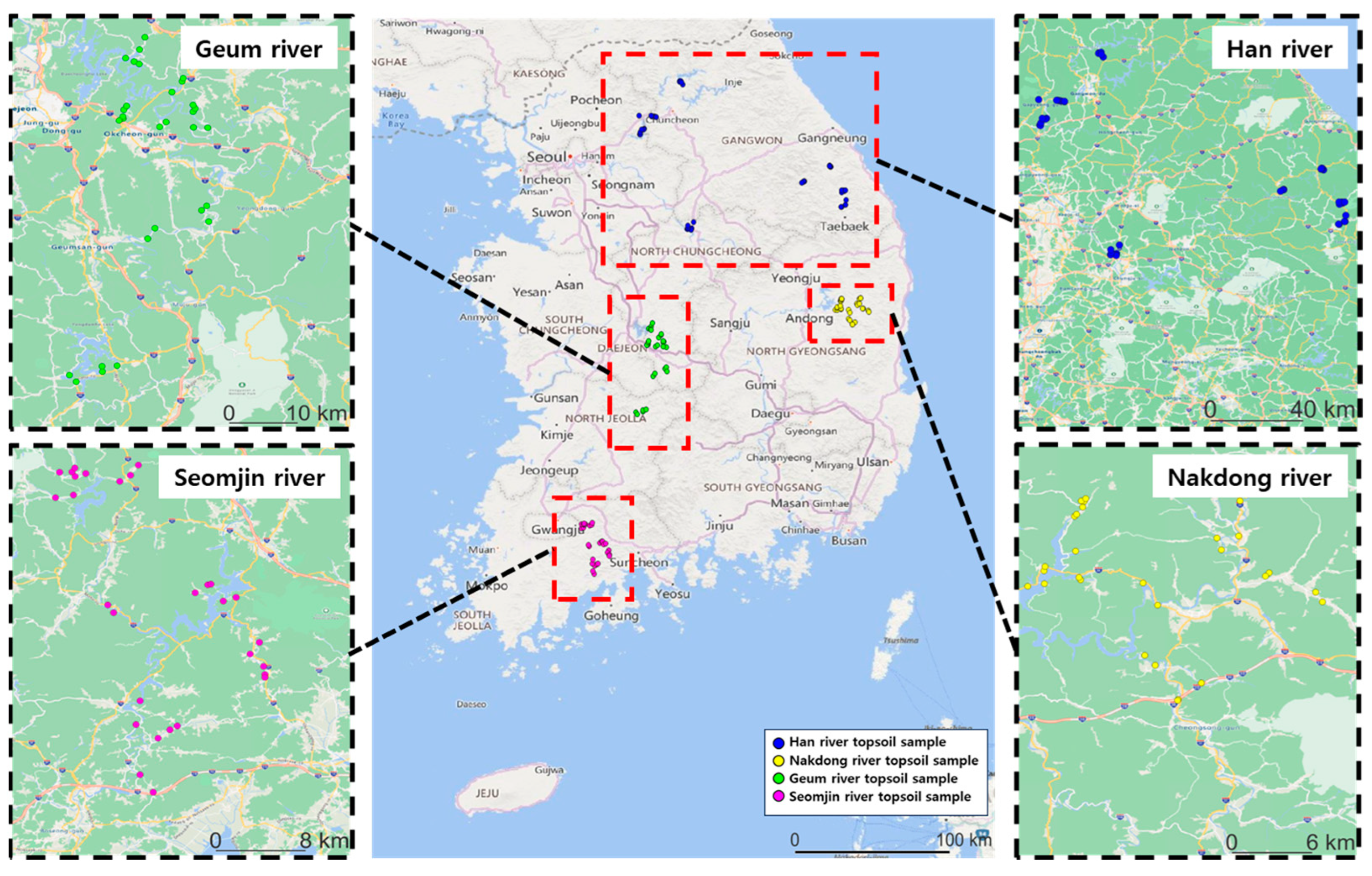
In 2020, topsoil samples were collected from 139 locations in the basins of four major rivers in the Republic of Korea. The Han River (HR), Nakdong River (NR), Seomjin River (SR), and Geum River (GR) are the four major river basins of the Republic of Korea. These basins are affected by surrounding land use and water quality, which can cause differences in the topsoil composition; thus, the areas where the samples were collected were classified [31]. Topsoil samples were collected at 50, 30, 29, and 30 points in the HR, NR, SR, and GR basins, respectively. These locations are shown in Figure 1. Topsoil samples from the HR, NR, SR, and GR were collected at locations up to 5800, 6400, 3200, and 2500 m from the river, respectively. Topsoil samples were collected in 1000 g using a hand auger at a depth of 10 to 15 cm after removing the 5 cm of the soil surface layer. Samples taken from five points in each area were mixed and homogenized as representative samples. The collected topsoil samples were brought to the laboratory, air-dried, and sieved through a 2 mm mesh to remove rock fragments and coarse roots [32].
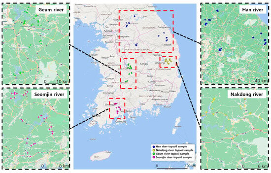
Figure 1.
Locations for topsoil sample collection.
The Kjeldahl method was used to determine the TN content in the topsoil samples [33]. The method comprises heating the topsoil sample to approximately 360 °C with concentrated sulfuric acid (H2SO4) and a catalyst until the topsoil turns white, distilling it with an automatic distillation device, and titrating it with a standard sulfuric acid solution [33].
2.2. Hyperspectral Imaging System
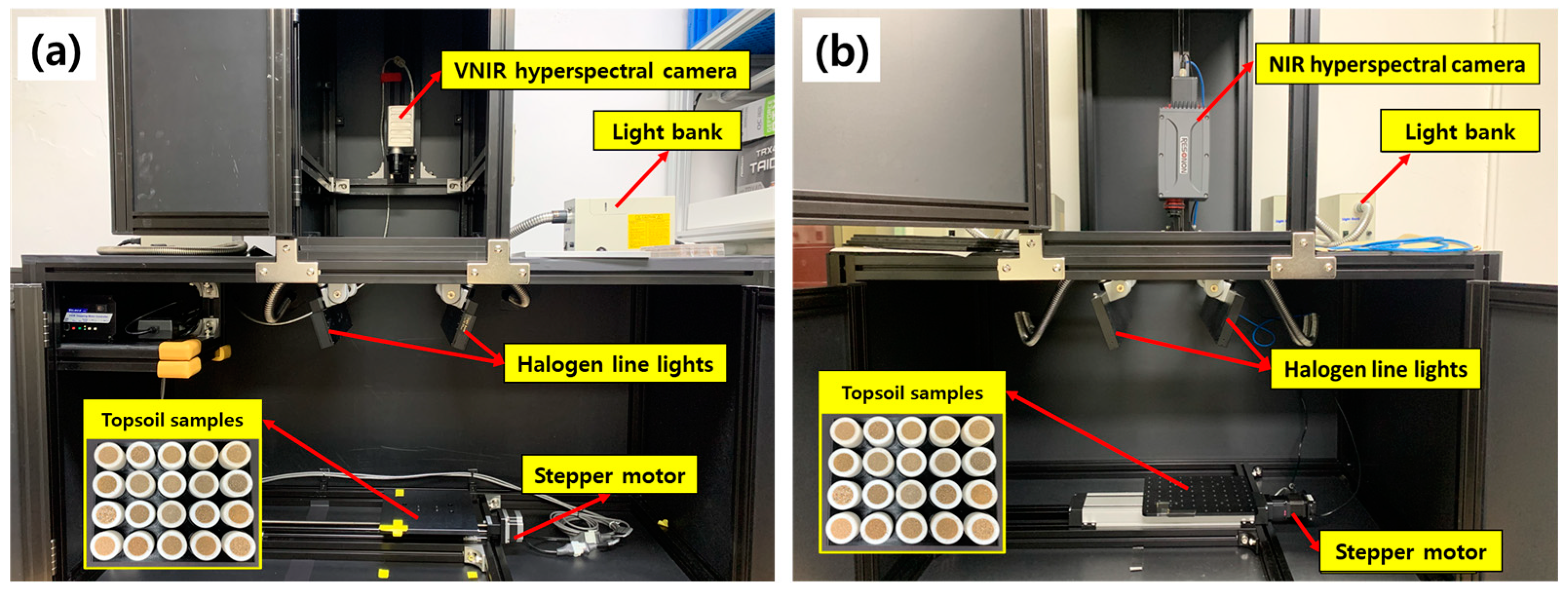
A hyperspectral imaging system consists of a hyperspectral imaging acquisition component, a light source, and a moving stage for the sample that is driven by a stepper motor. The experiment was conducted in a dark room to minimize noise in the spectra that could be caused by external light. Figure 2a shows a hyperspectral imaging system in the visible and near-infrared (VNIR) using a 12-bit line scan hyperspectral camera (micro HSI™ 410 Hyperspectral Sensor, Corning Inc., Corning, NY, USA) in the wavelength range of 400–1000 nm at a spectral resolution of 2 nm. Hyperspectral images of 300 bands were obtained. A pair of 100 W quartz tungsten halogen (QTH) line lights, fixed at 30° (zenith angle), were used for illumination. The vertical distance between the topsoil sample and the hyperspectral camera lens was set to 726 mm to prevent light saturation. The exposure time was set to 6 ms, and 135 lines were measured with the step interval of the moving stage set to 1 mm.
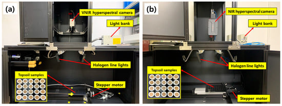
Figure 2.
(a) Visible to near-infrared (VNIR) and (b) near-infrared (NIR) hyperspectral imaging system used in the experiments.
Figure 2b shows a hyperspectral imaging system in the near-infrared (NIR) range using a 14-bit line-scan hyperspectral camera (Pika IR+, Resonon Inc., Bozeman, MT, USA) in the wavelength range of 895–1720 nm at a spectral resolution of 2.41 nm; hyperspectral images of 336 spectral bands were obtained. A pair of 100 W quartz tungsten halogen (QTH) line lights, tilted at 15° from vertical to excite the samples, were used for illumination. The vertical distance between the topsoil sample and the hyperspectral camera lens was set to 510 mm to prevent light saturation. The exposure time was set to 90 ms, and 650 lines were measured with the step interval of the moving stage set to 2.8 mm.
The HSI is dependent on the sample conditions, such as the degree of milling and height of the sample surface. Therefore, all HSI acquisitions were performed under the same conditions. The 139 topsoil samples were each placed in a Teflon container with an outer diameter of 30 mm, inner diameter of 20 mm, and depth of 15 mm. After removing the air gaps between the particles by applying pressure, the topsoil samples were flattened to obtain smooth surfaces of the same height; three sets of samples were created (Set A, Set B, and Set C). The vertical and horizontal axes of each line-scan image included the respective spectral and spatial information. The HSIs of 139 topsoil samples were measured three times at two-hour intervals under the same conditions. All experiments were performed three times for each set to acquire a total of 417 hyperspectral data per set.
2.3. Collection of Hyperspectral Image (HSI)
The HSIs of topsoil samples were calibrated according to Equation (1) using dark and white reference images. Dark reference images were obtained without light source exposure, and the white reference images were taken using diffuse reflectance standards of 99% (Labsphere, North Sutton, NH, USA) [34]. For each topsoil sample, the average and pixel spectra of the topsoil samples were extracted from the calibrated HSIs of the regions of interest (ROIs), excluding the container. The average spectrum was calculated as one reflectance spectrum, and all the pixels within each ROI were averaged. Approximately 600 and 1800 pixels were selected for the HSI of the average spectrum of each topsoil sample in the VNIR and NIR ranges, respectively. The HSI was extracted using MATLAB (version R2020a; Mathworks, Natick, MA, USA).
where I and Is are the corrected relative and sample hyperspectral images, respectively. Iw and D are the hyperspectral images of the white and dark reference plates, respectively, all of them at the ith wavelength.
2.4. Spectral Preprocessing
Various image spectrum preprocessing methods that correct the spectral shape distortion, light scattering, and device noise that may occur from the external environment were evaluated to improve the performance of the TN content prediction model [35,36]. The preprocessing of the reflectance spectra included smoothing (moving average), first-order and second-order derivatives, maximum normalization, mean normalization, range normalization, standard normal variate (SNV), and multiplicative scatter correction (MSC). The characteristics of the preprocessing and gap size set during the process are summarized in Table 1. The first- and second-order derivatives were analyzed by setting the gap size to three levels. Preprocessing of the reflectance spectra was performed using the Unscrambler X (Ver. 10.4, CAMO Software, Oslo, Norway).

Table 1.
Characteristics of preprocessing and applied gap size value.
2.5. Development of Total Nitrogen (TN) Content Prediction Models
Prediction models for TN content in topsoil were developed using PLSR and 1D-CNN, and the performance of each was compared. Three independent sample datasets (Set A, Set B, and Set C) were constructed from the 139 topsoil samples to develop the two models. To minimize the impact of errors that may occur during HSI measurements, hyperspectral data were collected on 139 topsoil samples three times, resulting in 417 hyperspectral spectral datasets per group. The dataset was classified into two subsets, a calibration dataset for developing the model (two sample dataset groups, Set A and Set B) and an independent test subset for prediction of the model (remaining sample dataset, Set C). The models were developed for the topsoil samples in the two-level wavelength ranges of 400–1000 nm (VNIR) and 895–1720 nm (NIR). The input data of the PLSR and the 1D-CNN models are HSI data, and the output data are the TN content of the topsoil.
2.5.1. Partial Least Squares Regression (PLSR)
The PLSR model is primarily applied to chemometrics and spectral data analysis. It determines linear combinations that consider variations in the predictor (x, spectrum) and response (y, soil properties) variables that describe a common structure [37]. To maximize the covariance between x and y, the PLSR algorithm incorporates successive regression and compression steps to obtain a set of orthogonal factors called latent variables (LVs). It then evaluates each model against a calibration set. The optimal factors for PLSR were determined using leave-one-out cross-validation (LOOCV) as the validation method [24,30,32]. A plot of the LOOCV residual variance versus the number of LVs was tested to specify the optimal number of LVs (called optimal factors) for PLSR. The optimal factors were obtained by minimizing the root mean squared error (RMSE) of the cross-validation.
The regression coefficients (b coefficients) were applied to determine the effective wavelength band using the PLSR model. When the b coefficient exceeded the thresholds, which were set to the standard deviation of the values, the corresponding wavelength was considered important [32,38]. The PLSR model was generated using the Unscrambler X software (Ver. 10.4, CAMO Software, Oslo, Norway). Table 2 lists the data used to develop and verify the PLSR model for predicting nitrogen content.

Table 2.
Datasets used to calibrate and predict PLSR models for predicting TN content in topsoil.
The PLS image obtained using the HSI was developed by applying the regression coefficients of the developed PLSR model [19].
2.5.2. One-Dimensional Convolutional Neural Networks (1D-CNNs)
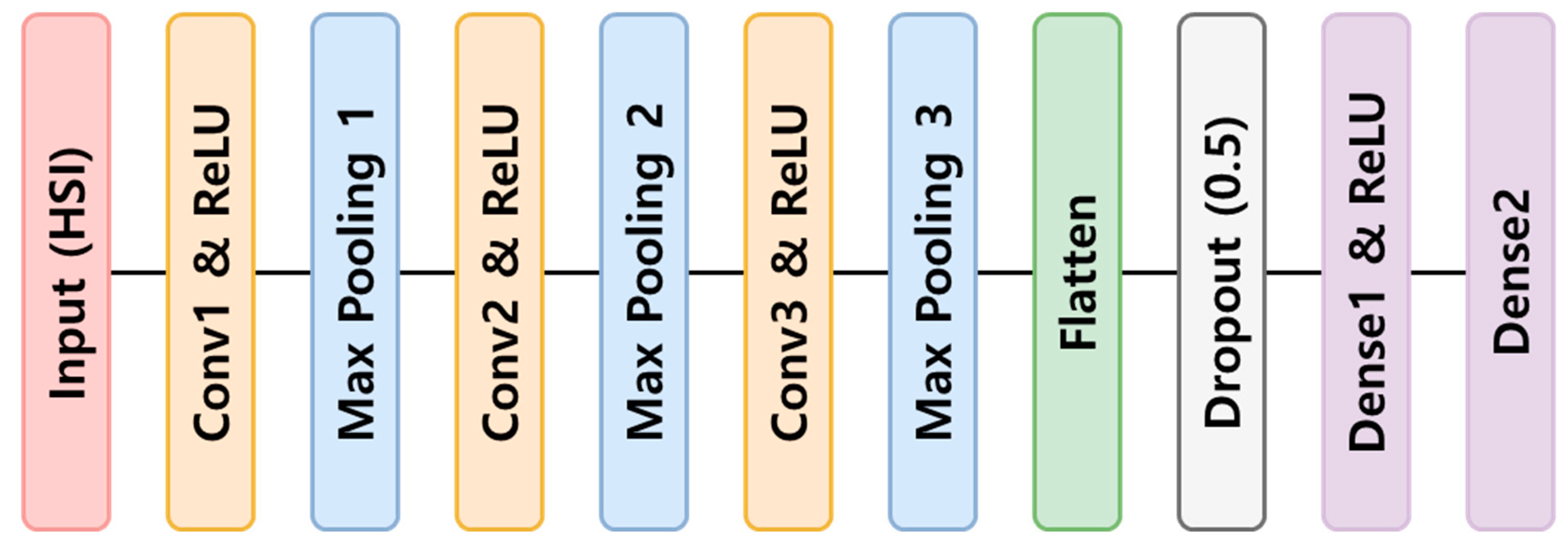
Although CNNs were initially proposed for image processing, they have recently also been adopted for extracting local abstract features from spectral data and establishing end-to-end models between the spectral data and target matrices [39,40]. CNN models are composed of convolution, pooling, and fully connected layers, and 1D-CNN models have input layers and 1D filters in the convolution layers that are suitable for 1D spectral data [41]. The depth of a CNN model increases as the number of convolutional layers increases, enabling the model to learn more abstract feature representations. However, if the layers are set incorrectly, information could be lost and performance could be degraded [25]. In this study, the 1D-CNN was organized into an input layer (Input), three convolution layers (Conv1, Conv2, and Conv3), three pooling layers (Max pooling1, Max pooling2, and Max pooling3), a flattened layer (Flatten), two fully connected layers (Dense1 and Dense2), and an output layer (Output) (Figure 3). The input and output data were the spectral data and TN content of the topsoil, respectively. The hyperparameters for each hidden layer are listed in Table 3. The convolution layer was set to 64 filters with a filter size of five. The pooling layer was set to apply max-pooling, which is an operation that subtracts the scalar value with the largest value from the result vector obtained from each convolution operation and is located in front of two fully connected layers with a pooling size of 3 and the number of strides equal to 2. The flattened layer converts a 1D multiple vector into a 1D single vector [25]. The activation function for all the hidden layers was the rectified linear unit (ReLU). A dropout rate of 0.5 was used to avoid overfitting.
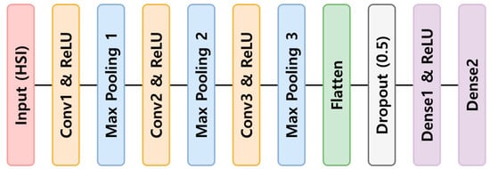
Figure 3.
One-dimensional neural convolutional network architecture.

Table 3.
Hyperparameters used in one-dimensional convolutional neural network (1D-CNN).
In general, a fixed-size spatial window in the HSI is used as the input data for the CNN model. However, this fixed-size architecture can decrease model performance because it ignores the various spatial information of the HSI, and insufficient HSI samples in 1D-CNN models may lead to overfitting [42]. The problem of insufficient learning samples was overcome by augmenting the amount of data by randomly selecting three levels (12.5, 25, and 50%) of the total number of pixels in the ROI area of each topsoil sample. The pixels selected were averaged and used as one spectral data point; this process was repeated 10 times. The number of pixels in the topsoil ROI at the VNIR wavelength was 600, and at 12.5, 25, and 50%, it was 75, 150, and 300, respectively. The number of pixels in the topsoil ROI at the NIR wavelength was 1800, and at 12.5, 25, and 50%, it was 225, 450, and 900, respectively. For the development and full cross-validation of the model for the two sets (Set A and Set B) of topsoil samples, 70% of the total data were randomly selected as a training dataset and 30% of the total data as the test dataset. The remaining topsoil sample set (Set C) not used for model development was used for model prediction. The number of data points in each dataset used for the development and prediction of the model is listed in Table 4. Adaptive moment estimation (Adam) was used as the optimization algorithm. The training conditions of the deep learning model were set to an epoch of 2000 and batch size of 64, and an early stop was set to a patience 20 to prevent model overfitting. The development and prediction of the 1D-CNN model were performed using the Python-based framework of Google Colab (Google LLC, Mountain View, CA, USA).

Table 4.
Datasets used to calibrate and predict 1D-CNN models for predicting TN content of topsoil.
2.5.3. Model Performance Evaluation
The actual TN content in the topsoil samples was compared with that predicted from the calibration (cross-validation) or independent validation datasets using the PLSR and 1D-CNN models. The performance of each model was evaluated by estimating the coefficient of determination of calibration set (Rc2), coefficient of determination of cross-validation set (Rv2), coefficient of determination of prediction set (Rp2), root mean squared error of calibration (RMSEC), root mean squared error of cross-validation (RMSEV), root mean squared error of prediction (RMSEP), and optimal factor (F) [32,43]. The data used for calibration and cross-validation were SET A and SET B of topsoil sample data, and the prediction data was SET C, topsoil sample data that were not used for model learning. The model with the highest Rv2 and lowest RMSEV was selected as the optimal model.
3. Results
3.1. TN Content of Topsoil Samples
Table 5 lists the minimum (Min), maximum (Max), average (Ave.), and standard deviation (Std.) values of the TN content in the basins of the four major rivers. The TN content of all 139 topsoil samples was in the range of 0.07–6.54 g kg−1, with an average of 1.33 g kg−1. The sample distribution range of Std. is an effective factor for determining model accuracy. The average TN content for the basins of the four major rivers was 1.72, 1.32, 1.22, and 1.09 g kg−1 for the SR, HR, GR, and NR basins, respectively. In the GR basin, the TN content (0.10–6.54 g kg−1) and standard deviation (1.18 g kg−1) were the highest.

Table 5.
TN content of topsoil samples from the basins of four major rivers in the Republic of Korea.
3.2. Topsoil Spectral Characteristics
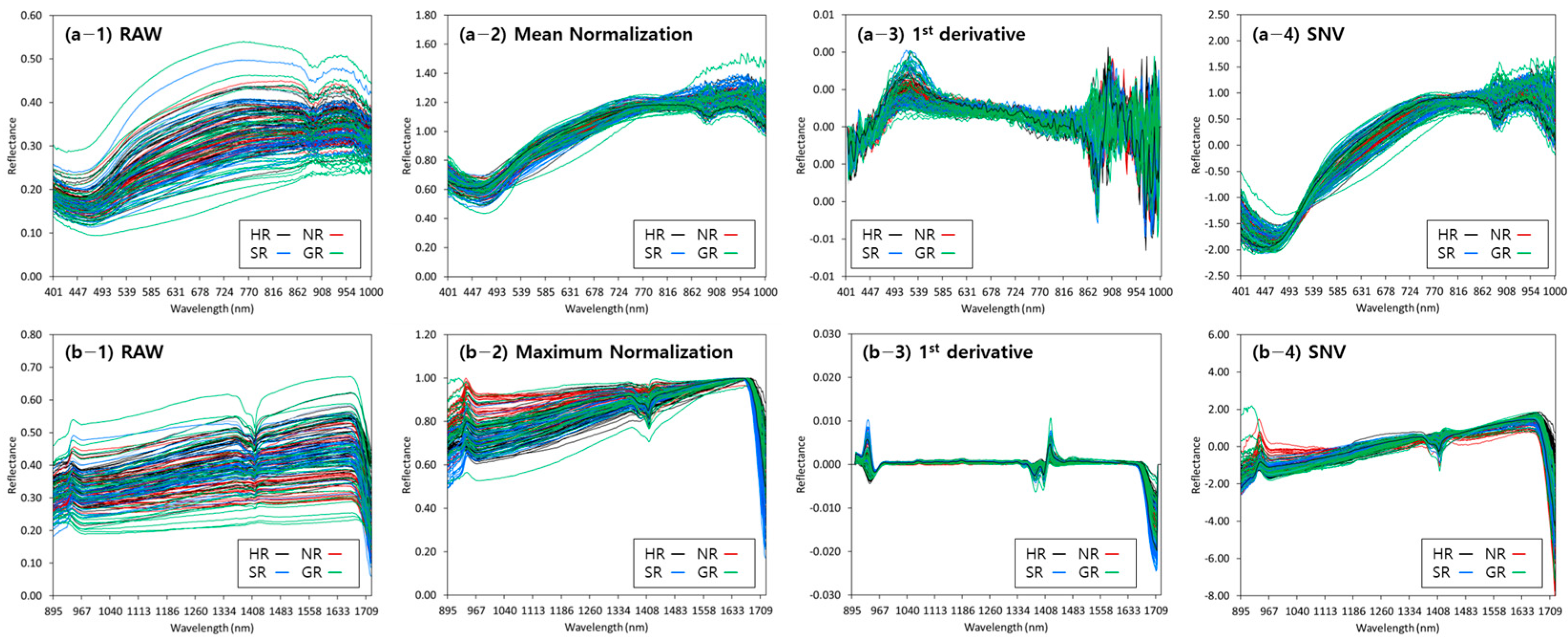
Figure 4 shows the raw reflection spectra of the topsoil samples and reflection spectra obtained by applying the main preprocessing methods. A difference in reflectance was observed in the raw spectrum depending on the origin of the sample; however, the spectral characteristics were similar. In the case of the spectrum without preprocessing, a sharp reflectance gradient after 450 nm and a relatively strong absorption band at approximately 894 nm were observed at the VNIR wavelength. These spectral characteristics are consistent with the results of previous studies [11,16]. When the spectrum was preprocessed with mean normalization (Figure 4(a-2)), Savitzky–Golay first-order derivatives (Figure 4(a-3)), and SNV (Figure 4(a-4)), strong absorption peaks were observed in the wavelength ranges of 460–490 nm and 894–900 nm, which are related to the presence of iron/iron oxides and soil organic matter (SOM). A previous study reported that other constituents may also act as spectrally active substitutes, such as clay minerals, and that spectrally featureless soil nitrogen may be related to these constituents [11]. For the spectrum without preprocessing, a positive peak at approximately 950 nm and a strong negative peak at approximately 1400 nm were observed at the NIR wavelength. The identified bands were relatively consistent (900–1000 nm) with previous findings for predictions of TN content in forest soils [44]. The topsoil reflectance spectrum is primarily attributed to a combination of weak overtones and fundamental vibrational bands coupled with C-H, N-H, and O-H, which may reflect the presence or absence of N protein, starch, and cellulose in the topsoil [44,45]. When the spectrum was preprocessed with maximum normalization (Figure 4(b-2)), Savitzky–Golay first-order derivatives (Figure 4(b-3)), and SNV in NIR (Figure 4(b-4)), a positive peak at approximately 950 nm and a strong negative peak at approximately 1400 nm were observed, similar to the raw spectrum. When the preprocessing of Savitzky–Golay first-order derivatives was applied, additional absorption peaks appeared at approximately 938, 1379, 1423, and 1710 nm (Figure 4(b-3)).

Figure 4.
(a) VNIR and (b) NIR reflectance of topsoil samples with applied main preprocessing ((1) raw, (2) normalization, (3) 1st derivative, and (4) SNV).
3.3. TN Content Prediction Model
3.3.1. Performance of the PLSR Model
A total of 130 PLSR models for predicting the TN content in topsoil samples from the basins of four major rivers were developed. The optimal models in the VNIR and NIR wavelength regions were selected by comparing the Rv2 and RMSEV values of the model (Table 6). Rv2 and RMSEV at the NIR wavelength were 0.736 and 0.45 g kg−1, respectively, which were higher than those at the VNIR wavelength (Rv2 = 0.658 and RMSEV = 0.51 g kg−1). The performance of the TN content prediction model improved when the model was developed by dividing the basins of the four major rivers by the 139 topsoil samples (total topsoil). For HR and SR, the TN content of the prediction models showed Rv2 values of 0.778 and 0.933, respectively, at the NIR wavelength, which were higher than those at the VNIR wavelength. In contrast, for NR and GR, the predicted Rv2 values of the TN content in the VNIR were 0.765 and 0.916, respectively. In NR, the performances in terms of TN content prediction for VNIR and NIR wavelengths were similar, in terms of Rv2 and RMSEV; however, the number of factors was small in VNIR, and compared to Rc2 and RMSEC, the model showed high performance at VNIR wavelengths.

Table 6.
Optimal model for TN content prediction (PLSR) in the basin of four major rivers.
The preprocessing methods were used to improve the prediction ability of PLSR. Hence, the prediction performance improved when the moving average and normalization preprocessing methods were applied, particularly when mean normalization was applied for the VNIR wavelength and maximum normalization was applied for the NIR wavelength. The optimal number of factors for the PLSR model was between 4 and 10 at VNIR wavelengths and between 13 and 16 at NIR wavelengths.
3.3.2. Performance of the 1D-CNN Model
From the total number of pixels in each topsoil sample, 12.5, 25, and 50% of the pixels were randomly selected, and the data were augmented 10 times. Subsequently, a 1D-CNN model for predicting the TN content of the topsoil was developed; its performance is presented in Table 7. As a result of developing a TN content prediction model using the entire ROI area (600 pixels) data of the VNIR wavelength, the Rv2 and RMSEV were 0.684 and 0.55 g kg−1, respectively, and as a result of validation with an unknown sample, Rp2 and RMSEP were 0.651 and 0.51 g kg−1, respectively. Verifying the model obtained by randomly selecting 25% (150 pixels) of the entire ROI area, resulted in a high predictive performance compared to that with 50 and 12.5% of the total ROI area. As a result of verifying the model obtained by randomly selecting 25% (150 pixels) of the entire ROI area, Rp2 and RMSEP were 0.84 and 0.34 g kg−1, respectively. This is a better prediction performance compared to that with 50% and 12.5% of the total ROI area. For a TN content prediction model using the entire ROI area (600 pixels) data for the NIR wavelength, an Rv2 and RMSEV of 0.360 and 0.78 g kg−1 were obtained, respectively, and for the validation with an unknown sample, Rp2 and RMSEP of 0.334 and 0.71 g kg−1 were obtained, respectively. The performance of the 1D-CNN model was improved by spectral data augmentation. Among them, the Rp2 and RMSEP of the prediction model obtained by randomly selecting 50% (900 pixels) of the entire ROI area were 0.93 and 0.23 g kg−1, respectively, which is a better performance compared to the other models. The Rv2 and RMSEV of the model that randomly selected 25% (450 pixels) of the ROI area were 0.887 and 0.29 g kg-1, respectively. For the same model, the Rp2 and RMSEP values were 0.816 and 0.37 g kg−1, which showed better verification results than the other models. Therefore, 450 pixels were selected for the next set of experimental data.

Table 7.
Comparison of the performances of the 1D-CNN models for predicting the TN content in the basin of four major rivers according to ROI size.
By comparing the TN content prediction performance according to the number of pixels, 150 pixels in the VNIR wavelength range and 450 pixels in the NIR wavelength range were selected as optimal sizes. Using these data, 130 1D-CNN models were developed by applying preprocessing to determine the TN content in the topsoil samples of the four major river basins. The performance of the developed model was evaluated by estimating Rv2 and RMSEV (Table 8). The optimal model was determined by comparing Rv2 and RMSEV, and the optimal preprocessing for each wavelength region was selected for the model. The Rv2 of the 1D-CNN models showed a high accuracy of 0.95 or higher, and the prediction performance was higher than that of the PLSR model. The performance of the 1D-CNN model for the total topsoil showed Rv2 and RMSEV values of 0.982 and 0.11 g kg−1 in the NIR wavelength, respectively, which were higher than those in the VNIR wavelength (Rv2 = 0.954 and RMSEV = 0.19 g kg−1). For the HR, NR, SR, and GR basins, the prediction models showed Rv2 values of 0.978, 0.972, 0.986, and 0.994, respectively, at the NIR wavelength, which were higher than those at the VNIR wavelength. In the NR, there was no difference between Rv2 and RMSEV in the VNIR and NIR ranges; however, Rp2 was high for the VNIR wavelength. Therefore, the prediction performance was considered excellent for the VNIR wavelength.

Table 8.
Optimal prediction model (1D-CNN) for TN content in the basin of four major rivers.
The results showed that various preprocessing techniques had a considerable effect on the performance of the 1D-CNN models. The performance of the model was improved by the preprocessing methods of the moving average, Savitzky–Golay first-order derivatives, and SNV. Topsoil, containing complex organic matter, has nonspecific spectral characteristics owing to overlapping absorption and low concentrations of soil components [30].
3.4. Regression Coefficient of the PLSR Model
Figure 5 shows the regression coefficient that could determine the effective wavelength in the optimal PLSR model for predicting the TN content in the river basins under consideration. A positive or negative regression coefficient was considered an effective wavelength for explaining the variation in the topsoil parameters when the standard deviation exceeded the set threshold (dashed line). For the VNIR wavelengths, a similar range of effective wavelengths was selected for the PLSR model to predict the total TN content in the total and GR samples. The PLSR model for the total and GR samples had significant positive peaks for the TN content at approximately 540–585, 844–880, and 913–970 nm, and negative peaks at approximately 712–770 nm (Figure 5a). For the PLSR for the HR, the regression coefficients at 435–436, 517–555, 613–633, 766–815, 862, 876, 944, 968, and 976 nm were significant. For the HR, the regression coefficient value after approximately 830 nm shows large fluctuations. The peak values were similar for each selected PLSR model in the NIR wavelength (Figure 5b). The selected effective wavelengths were 1380–1430 nm, 1470–1560 nm, and 1670–1681 nm. In the remaining models, except for the HR, the selected effective wavelengths were those less than approximately 943 nm and in the range 1310–1350 nm. The PLSR model in the total and GR samples had significant positive peaks for TN content at approximately 960–984 nm.

Figure 5.
Plots of the regression coefficient with the PLSR models for TN content predictions in (1) Total, (2) Han River, (3) Nakdong River, (4) Seomjin River, and (5) Geum River samples under the (a) VNIR (400–1000 nm) and (b) NIR (895–1720 nm).
PLS images were obtained by applying PLSR regression coefficients to topsoil HSI (Figure 6). HSI images have reflectance data for 300 wavelength bands in the VNIR and 336 wavelength bands in the NIR for each pixel. HSI revealed different reflectance even within the same topsoil sample. A binarized image was obtained by removing the background of HSI at a specific wavelength, and then a threshold was applied to the binarized image to map the TN content of the topsoil. The developed PLS model was applied to HSI to obtain a PLS image, which is a topsoil nitrogen prediction map. As shown in Figure 6, PLS images were confirmed to be a potential technology that can visualize and represent the TN content of topsoil.

Figure 6.
PLS image acquisition steps representing topsoil TN content from hyperspectral images (example of PLS image by applying topsoil TN prediction model developed in NIR wavelength).
3.5. Performance Evaluation of the Optimal Model for Predicting TN Content in Topsoil
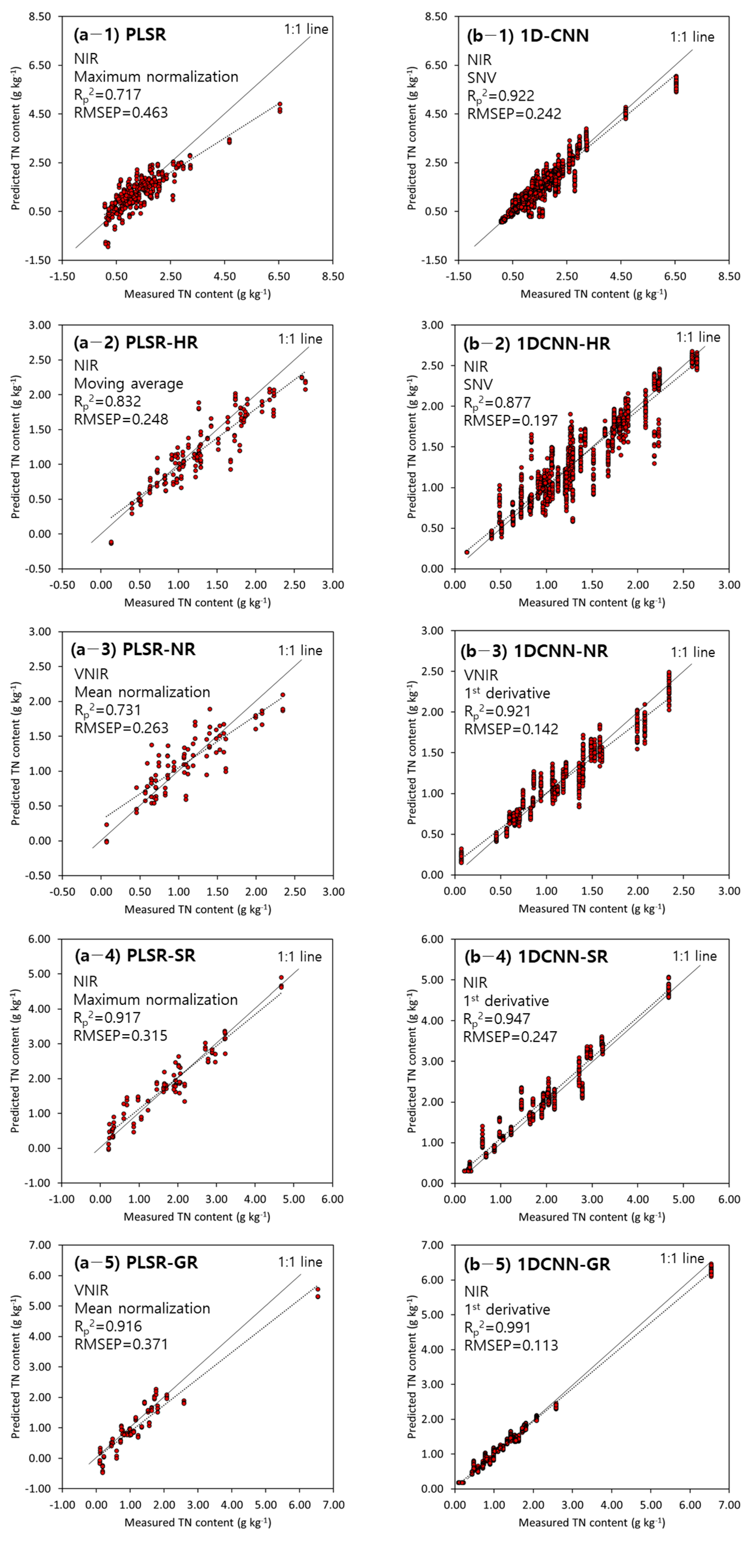
The developed optimal model for predicting TN content in the topsoil from each of the four major river basins was verified using a prediction dataset that was not used to develop the model (Figure 7). The 1D-CNN model was superior to the PLSR model. The Rp2 values of the optimal PLSR (with maximum normalization preprocessing) and 1D-CNN (with SNV preprocessing) models were 0.72 and 0.92, respectively. The performance of the PLSR model for TN content prediction improved for each of the four major rivers, with Rp2 ranging from 0.832 to 0.917 (Figure 7a). When the TN content in topsoil for each of the four major rivers was predicted using the 1D-CNN, the Rp2 of the 1D-CNN model ranged from 0.877 to 0.991 and RMSE ranged from 0.113 to 0.247 g kg−1, which were similar to or better than those of the prediction model for TN content in topsoil (Figure 7b). The prediction of the TN content in topsoil in the basins of the four rivers showed higher performance at NIR wavelengths (excluding Nakdong River).
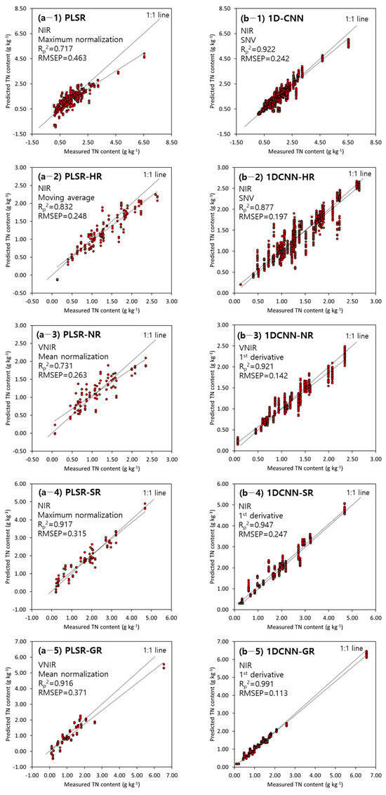
Figure 7.
Scatter plot of predicted vs. measured TN content in each of the four major rivers in the prediction dataset for the optimal model: (a) PLSR model, (b) 1D-CNN model, (1) Total, (2) Han River, (3) Nakdong River, (4) Seomjin River, and (5) Geum River. (The solid line represents a 1:1 line and the dotted line represents the trend line of the data).
4. Discussion
The results of this study show that there is potential for predicting TN content in topsoil using HSI. The PLSR and 1D-CNN models in this study could be applied to estimate topsoil TN content in the range of 0.07–6.54 g kg−1. The prediction performance improved when the spectral preprocessing methods were applied. Therefore, the various preprocessing methods for spectra can successfully eliminate the effects of high-frequency noise, such as the light-scattering effect of particles of different sizes and shapes [23]. The prediction accuracy of the 1D-CNN model improved when Savitzky–Golay first-order derivatives and SNV preprocessing were applied. The results of this experiment are similar to those of previous studies, which reported that, for most machine learning techniques, the Savitzky–Golay transformation (including the first derivative, second derivative, and smoothing) is more effective than other preprocessing methods [11].
The regression coefficient of the PLSR model that could determine the effective wavelength was compared. Previous studies have reported nitrogen-sensitive bands at wavelengths of 451–491, 511–521, 536, 612–658, 980–997, 1209–1376, and 1472–1795 nm [10]. The results of this study are consistent with those of previous studies that reported that 985, 991, 1010, and 1490 nm are the main wavelengths for TN content identification [21]. The wavelength in the band near 1000 nm may be associated with 3v1 N-H, and that near 1850 nm may be associated with 4v1 C-H [46].
The results of the PLSR and 1D-CNN models indicate higher or similar accuracy compared to those of previous studies (Figure 6) [10,11,23,40]. Vibhute et al. [10] reported that when the TN content in the topsoil was predicted using the PLSR model, Rp2 was 0.64–0.94 and RMSEP was 1.56–4.34 mg kg−1. Yuan et al. [40] developed a 1D-CNN model by applying NIR spectral data to predict the TN in topsoil and reported that the R2 and RMSE were 0.72 and 0.66 g kg−1, respectively. Xu et al. [11] reported that the Rp2 and RMSEP of the TN prediction support vector machine regression model using HSI were 0.94 and 0.17 g kg−1, respectively. HSIs have more information about the topsoil space compared to existing spectral data, so it is concluded that the performance of the models was better compared to the results of previous studies.
Some studies report that in machine learning, models must be developed carefully because of the risk of over-fitting predictions to irrelevant elements of the spectrum [11,47,48,49]. Large-scale topsoil profiles need to be built to prevent overfitting in machine learning and estimate complex properties of the topsoil. This means that a variety of topsoil types and geographic samples are essential to make machine learning more generalizable [48]. However, this study is limited in that large-scale topsoil profiles are required to apply this model to remote sensing. Additionally, techniques such as spectral variable selection techniques and uninformative algorithm removal should be utilized to develop simplified machine learning [11,47]. dos Santos et al. [49] predicted SOC using a cross-validation (CV) strategy oriented to soil profiles and improved model interpretability by using the least absolute shrinkage and selection operator (LASSO) regression method. Selecting the effective wavelength variable might improve model performance and reduce computational time.
5. Conclusions
This study focused on evaluating the feasibility of hyperspectral images for assessing the TN content in topsoil and developing a model for the prediction of TN content based on machine learning models. The PLSR and 1D-CNN models were developed by applying preprocessing, which minimized the discrimination error due to spectral overlap and improved the performance of the model. The optimal model was determined by applying eight spectral preprocessing methods in two wavelength ranges to determine the optimal conditions for the highest performance of TN content prediction.
The prediction model for TN content (with overall TN contents ranging from 0.07 to 6.54 g kg−1) using the HSI reflectance spectrum showed a high prediction performance in the NIR wavelength. In addition, the deep-learning-based 1D-CNN model was superior to the PLSR model in predicting the TN content in topsoil. Data augmentation improved the performance of the 1D-CNN model (Rp2 = 0.922 and RMSEP = 0.242 g kg−1 in total topsoil). The performance of the TN content prediction model could be improved by applying moving average, normalization, Savitzky–Golay first-order derivatives, and SNV preprocessing methods.
This study confirmed that the chemical properties of topsoil can be rapidly predicted using HSI. In the future, combining these results with remote sensing technology is expected to help develop topsoil nitrogen content mapping profiles.
Author Contributions
All authors contributed to the manuscript preparation. Conceptualization, M.-J.K., J.-E.L. and C.M.; formal analysis, M.-J.K. and J.-E.L.; investigation, M.-J.K. and J.-E.L.; resources, M.-J.K. and J.-E.L.; software, I.B.; writing—original draft preparation, M.-J.K.; writing—review and editing, C.M.; visualization, M.-J.K.; supervision, C.M.; project administration, K.J.L. and C.M.; funding acquisition, K.J.L. and C.M. All authors have read and agreed to the published version of the manuscript.
Funding
This work was supported by the Ministry of Environment of Korea as The SS (Surface Soil conservation and management) project (2019002820003).
Institutional Review Board Statement
Not applicable.
Data Availability Statement
Not applicable.
Conflicts of Interest
The authors declare no conflict of interest.
References
- Lim, Y.; Kim, S.; Nam, S.; Chun, K.; Kim, M. A Comparison of Current Trends in Soil Erosion Research Using Keyword Co-occurrence Analysis. Korean J. Environ. Ecol. 2020, 34, 413–424. [Google Scholar] [CrossRef]
- Holz, D.J.; Williard, K.W.J.; Edwards, P.J.; Schoonover, J.E. Soil Erosion in Humid Regions: A Review. J. Contemp. Water Res. Educ. 2015, 154, 48–59. [Google Scholar] [CrossRef]
- Conforti, M.; Matteucci, G.; Buttafuoco, G. Using laboratory Vis-NIR spectroscopy for monitoring some forest soil properties. J. Soils Sediments 2018, 18, 1009–1019. [Google Scholar] [CrossRef]
- Morellos, A.; Pantazi, X.E.; Moshou, D.; Alexandridis, T.; Whetton, R.; Tziotzios, G.; Wiebensohn, J.; Bill, R.; Mouazen, A.M. Machine learning based prediction of soil total nitrogen, organic carbon and moisture content by using VIS-NIR spectroscopy. Biosyst. Eng. 2016, 152, 104–116. [Google Scholar] [CrossRef]
- Lee, J.-H. Derivation of regional annual mean rainfall erosivity for predicting topsoil erosion in Korea. J. Korea Water Resour. Assoc. 2018, 51, 783–793. [Google Scholar] [CrossRef]
- Lee, K.; Sung, H.C.; Seo, J.Y.; Yoo, Y.; Kim, Y.; Kook, J.H.; Jeon, S.W. The Integration of Remote Sensing and Field Surveys to Detect Ecologically Damaged Areas for Restoration in South Korea. Remote Sens. 2020, 12, 3687. [Google Scholar] [CrossRef]
- Lee, J.; Lee, S.; Hong, J.; Lee, D.; Bae, J.H.; Yang, J.E.; Kim, J.; Lim, K.J.; Lee, J.; Lee, S.; et al. Evaluation of Rainfall Erosivity Factor Estimation Using Machine and Deep Learning Models. Water 2021, 13, 382. [Google Scholar] [CrossRef]
- Jeong, G. Evaluating Spectral Preprocessing Methods for Visible and Near Infrared Reflectance Spectroscopy to Predict Soil Carbon and Nitrogen in Mountainous Areas. J. Korean Geogr. Soc. 2016, 51, 509–523. [Google Scholar]
- Datta, D.; Paul, M.; Murshed, M.; Teng, S.W.; Schmidtke, L. Soil Moisture, Organic Carbon, and Nitrogen Content Prediction with Hyperspectral Data Using Regression Models. Sensors 2022, 22, 7998. [Google Scholar] [CrossRef]
- Vibhute, A.D.; Kale, K.V.; Gaikwad, S.V.; Dhumal, R.K. Estimation of soil nitrogen in agricultural regions by VNIR reflectance spectroscopy. SN Appl. Sci. 2020, 2, 1523. [Google Scholar] [CrossRef]
- Xu, S.; Wang, M.; Shi, X.; Yu, Q.; Zhang, Z. Integrating hyperspectral imaging with machine learning techniques for the high-resolution mapping of soil nitrogen fractions in soil profiles. Sci. Total Environ. 2021, 754, 142135. [Google Scholar] [CrossRef] [PubMed]
- Jwaideh, M.A.A.; Sutanudjaja, E.H.; Dalin, C. Global impacts of nitrogen and phosphorus fertiliser use for major crops on aquatic biodiversity. Int. J. Life Cycle Assess. 2022, 27, 1058–1080. [Google Scholar] [CrossRef]
- Balasuriya, B.T.G.; Ghose, A.; Gheewala, S.H.; Prapaspongsa, T. Assessment of eutrophication potential from fertiliser application in agricultural systems in Thailand. Sci. Total Environ. 2022, 833, 154993. [Google Scholar] [CrossRef]
- de Santana, F.B.; de Souza, A.M.; Poppi, R.J. Green methodology for soil organic matter analysis using a national near infrared spectral library in tandem with learning machine. Sci. Total Environ. 2019, 658, 895–900. [Google Scholar] [CrossRef] [PubMed]
- Choe, E.; Hong, S.Y.; Kim, Y.; Song, K.; Zhang, Y. Quantification of Soil Properties using Visible-NearInfrared Reflectance Spectroscopy. Korean J. Soil Sci. Fertil. 2009, 42, 522–528. [Google Scholar]
- Ma, J.; Cheng, J.; Wang, J.; Pan, R.; He, F.; Yan, L.; Xiao, J. Rapid detection of total nitrogen content in soil based on hyperspectral technology. Inf. Process. Agric. 2022, 9, 566–574. [Google Scholar] [CrossRef]
- Pudełko, A.; Chodak, M. Estimation of total nitrogen and organic carbon contents in mine soils with NIR reflectance spectroscopy and various chemometric methods. Geoderma 2020, 368, 114306. [Google Scholar] [CrossRef]
- Peng, Y.; Zhao, L.; Hu, Y.; Wang, G.; Wang, L.; Liu, Z. Prediction of soil nutrient contents using visible and near-infrared reflectance spectroscopy. ISPRS Int. J. Geo-Inf. 2019, 8, 437. [Google Scholar] [CrossRef]
- Kim, M.J.; Lim, J.; Kwon, S.W.; Kim, G.; Kim, M.S.; Cho, B.K.; Baek, I.; Lee, S.H.; Seo, Y.; Mo, C. Geographical origin discrimination of white rice based on image pixel size using hyperspectral fluorescence imaging analysis. Appl. Sci. 2020, 10, 5794. [Google Scholar] [CrossRef]
- Gomez, C.; Lagacherie, P.; Coulouma, G. Regional predictions of eight common soil properties and their spatial structures from hyperspectral Vis-NIR data. Geoderma 2012, 189–190, 176–185. [Google Scholar] [CrossRef]
- Sorenson, P.T.; Quideau, S.A.; Rivard, B. High resolution measurement of soil organic carbon and total nitrogen with laboratory imaging spectroscopy. Geoderma 2018, 315, 170–177. [Google Scholar] [CrossRef]
- Yu, H.; Kong, B.; Wang, G.; Du, R.; Qie, G. Prediction of soil properties using a hyperspectral remote sensing method. Arch. Agron. Soil Sci. 2018, 64, 546–559. [Google Scholar] [CrossRef]
- Qi, H.; Paz-Kagan, T.; Karnieli, A.; Jin, X.; Li, S. Evaluating calibration methods for predicting soil available nutrients using hyperspectral VNIR data. Soil Tillage Res. 2018, 175, 267–275. [Google Scholar] [CrossRef]
- Alomar, S.; Mireei, S.A.; Hemmat, A.; Masoumi, A.A.; Khademi, H. Comparison of Vis/SWNIR and NIR spectrometers combined with different multivariate techniques for estimating soil fertility parameters of calcareous topsoil in an arid climate. Biosyst. Eng. 2021, 201, 50–66. [Google Scholar] [CrossRef]
- Yu, G.; Ma, B.; Chen, J.; Li, X.; Li, Y.; Li, C. Nondestructive identification of pesticide residues on the Hami melon surface using deep feature fusion by Vis/NIR spectroscopy and 1D-CNN. J. Food Process Eng. 2021, 44, e13602. [Google Scholar] [CrossRef]
- Vohland, M.; Besold, J.; Hill, J.; Fründ, H.C. Comparing different multivariate calibration methods for the determination of soil organic carbon pools with visible to near infrared spectroscopy. Geoderma 2011, 166, 198–205. [Google Scholar] [CrossRef]
- Jung, A.; Vohland, M.; Thiele-Bruhn, S. Use of a portable camera for proximal soil sensing with hyperspectral image data. Remote Sens. 2015, 7, 11434–11448. [Google Scholar] [CrossRef]
- Zhang, T.; Li, L.; Zheng, B. Estimation of agricultural soil properties with imaging and laboratory spectroscopy. J. Appl. Remote Sens. 2013, 7, 073587. [Google Scholar] [CrossRef]
- Šestak, I.; Mihaljevski Boltek, L.; Mesić, M.; Zgorelec, Ž.; Perčin, A. Hyperspectral sensing of soil ph, total carbon and total nitrogen content based on linear and non-linear calibration methods. J. Cent. Eur. Agric. 2019, 20, 504–523. [Google Scholar] [CrossRef]
- Xu, S.; Zhao, Y.; Wang, M.; Shi, X. Comparison of multivariate methods for estimating selected soil properties from intact soil cores of paddy fields by Vis–NIR spectroscopy. Geoderma 2018, 310, 29–43. [Google Scholar] [CrossRef]
- Kang, D.; Sung, K.; Yeo, U.; Chung, Y.; Lee, S.-M. Riparian Area Characteristics of the Middle and Lower Reaches of the Nakdong River, Korea Riparian Area Characteristics of the Middle and Lower Reaches of the Nakdong River, Korea. J. Environ. Impact Assess. 2008, 17, 189–200. [Google Scholar]
- Kim, M.J.; Lee, H.I.; Choi, J.H.; Lim, K.J.; Mo, C. Development of a Soil Organic Matter Content Prediction Model Based on Supervised Learning Using Vis-NIR/SWIR Spectroscopy. Sensors 2022, 22, 5129. [Google Scholar] [CrossRef] [PubMed]
- Bremner, J.M. Determination of nitrogen in soil by the Kjeldahl method. J. Agric. Sci. 1960, 55, 11–33. [Google Scholar] [CrossRef]
- Kim, W.-K.; Hong, S.-J.; Cui, J.; Kim, H.-J.; Park, J.; Yang, S.-H.; Kim, G. Application of NIR Spectroscopy and Artificial Neural Network Techniques for Real-Time Discrimination of Soil Categories. J. Korean Soc. Nondestruct. Test. 2017, 37, 148–157. [Google Scholar] [CrossRef]
- Barra, I.; Haefele, S.M.; Sakrabani, R.; Kebede, F. Soil spectroscopy with the use of chemometrics, machine learning and pre-processing techniques in soil diagnosis: Recent advances—A review. TrAC Trends Anal. Chem. 2021, 135, 116166. [Google Scholar] [CrossRef]
- Tiecher, T.; Moura-Bueno, J.M.; Caner, L.; Minella, J.P.G.; Evrard, O.; Ramon, R.; Naibo, G.; Barros, C.A.P.; Silva, Y.J.A.B.; Amorim, F.F.; et al. Improving the quantification of sediment source contributions using different mathematical models and spectral preprocessing techniques for individual or combined spectra of ultraviolet–visible, near- and middle-infrared spectroscopy. Geoderma 2021, 384, 114815. [Google Scholar] [CrossRef]
- Geladi, P.; Kowalski, B.R. Partial least-squares regression: A tutorial. Anal. Chim. Acta 1986, 185, 1–17. [Google Scholar] [CrossRef]
- Kiala, Z.; Odindi, J.; Mutanga, O.; Peerbhay, K. Comparison of partial least squares and support vector regressions for predicting leaf area index on a tropical grassland using hyperspectral data. J. Appl. Remote Sens. 2016, 10, 036015. [Google Scholar] [CrossRef]
- Zhang, X.; Yang, J.; Lin, T.; Ying, Y. Food and agro-product quality evaluation based on spectroscopy and deep learning: A review. Trends Food Sci. Technol. 2021, 112, 431–441. [Google Scholar] [CrossRef]
- Yuan, Q.; Wang, J.; Zheng, M.; Wang, X. Hybrid 1D-CNN and attention-based Bi-GRU neural networks for predicting moisture content of sand gravel using NIR spectroscopy. Constr. Build. Mater. 2022, 350, 128799. [Google Scholar] [CrossRef]
- Kawamura, K.; Nishigaki, T.; Andriamananjara, A.; Rakotonindrina, H.; Tsujimoto, Y.; Moritsuka, N.; Rabenarivo, M.; Razafimbelo, T. Using a one-dimensional convolutional neural network on visible and near-infrared spectroscopy to improve soil phosphorus prediction in Madagascar. Remote Sens. 2021, 13, 1519. [Google Scholar] [CrossRef]
- Feng, J.; Wang, L.; Yu, H.; Jiao, L.; Zhang, X. Divide-and-conquer dual-architecture convolutional neural network for classification of hyperspectral images. Remote Sens. 2019, 11, 484. [Google Scholar] [CrossRef]
- Roger, J.M.; Chauchard, F.; Bellon-Maurel, V. EPO-PLS external parameter orthogonalisation of PLS application to temperature-independent measurement of sugar content of intact fruits. Chemom. Intell. Lab. Syst. 2003, 66, 191–204. [Google Scholar] [CrossRef]
- Tahmasbian, I.; Xu, Z.; Boyd, S.; Zhou, J.; Esmaeilani, R.; Che, R.; Hosseini Bai, S. Laboratory-based hyperspectral image analysis for predicting soil carbon, nitrogen and their isotopic compositions. Geoderma 2018, 330, 254–263. [Google Scholar] [CrossRef]
- Rodríguez-Pérez, J.R.; Marcelo, V.; Pereira-Obaya, D.; García-Fernández, M.; Sanz-Ablanedo, E. Estimating Soil Properties and Nutrients by Visible and Infrared Diffuse Reflectance Spectroscopy to Characterize Vineyards. Agronomy 2021, 11, 1895. [Google Scholar] [CrossRef]
- Yang, H.; Kuang, B.; Mouazen, A.M. Quantitative analysis of soil nitrogen and carbon at a farm scale using visible and near infrared spectroscopy coupled with wavelength reduction. Eur. J. Soil Sci. 2012, 63, 410–420. [Google Scholar] [CrossRef]
- Raj, A.; Chakraborty, S.; Duda, B.M.; Weindorf, D.C.; Li, B.; Roy, S.; Sarathjith, M.C.; Das, B.S.; Paulette, L. Soil mapping via diffuse reflectance spectroscopy based on variable indicators: An ordered predictor selection approach. Geoderma 2018, 314, 146–159. [Google Scholar] [CrossRef]
- Viscarra Rossel, R.A.; Behrens, T.; Ben-Dor, E.; Chabrillat, S.; Demattê, J.A.M.; Ge, Y.; Gomez, C.; Guerrero, C.; Peng, Y.; Ramirez-Lopez, L.; et al. Diffuse reflectance spectroscopy for estimating soil properties: A technology for the 21st century. Eur. J. Soil Sci. 2022, 73, e13271. [Google Scholar] [CrossRef]
- dos Santos, E.P.; Moreira, M.C.; Fernandes-Filho, E.I.; Demattê, J.A.M.; dos Santos, U.J.; da Silva, D.D.; Cruz, R.R.P.; Moura-Bueno, J.M.; Santos, I.C.; de Sá Barreto Sampaio, E.V. Improving the generalization error and transparency of regression models to estimate soil organic carbon using soil reflectance data. Ecol. Inform. 2023, 77, 102240. [Google Scholar] [CrossRef]
Disclaimer/Publisher’s Note: The statements, opinions and data contained in all publications are solely those of the individual author(s) and contributor(s) and not of MDPI and/or the editor(s). MDPI and/or the editor(s) disclaim responsibility for any injury to people or property resulting from any ideas, methods, instructions or products referred to in the content. |
© 2023 by the authors. Licensee MDPI, Basel, Switzerland. This article is an open access article distributed under the terms and conditions of the Creative Commons Attribution (CC BY) license (https://creativecommons.org/licenses/by/4.0/).

