Abstract
The incorporation of biodegraded substrates during the germination of horticultural crops has shown favorable responses in different crops; however, most of these studies evaluate their effect only in the first days of seedling life, and do not follow up on the production process under greenhouse or open field conditions. The objective of this study was to evaluate the phenological development of Lycopersicon esculetum (tomato) seedlings in greenhouses that were germinated with biodegraded substrate mixed with peat moss. To find the best plant performance condition and determine whether the biodegraded substrate allows tomato plants to be obtained with the conditions for their production, the response surface methodology (RSM) and artificial neural network (ANN) were used. Three response surface models and three neural network models were developed to analyze the plant growth, the leaf length and the leaf width. The results obtained show that plant height during the first days presented statistically significant differences among the different treatments, with an initial average height of 5.3 cm. The length of the leaves at transplantation was statistically different, maintaining a length of 2.4, and the width of the leaves at transplantation measured 1.8 cm. The RSM and ANN models allowed the estimation of the optimal value of the adequate amount of degraded substrate to germinate Lycopersicon esculetum and reduce the use of peat moss. The coefficient of determination (r2) indicates that the ANNs presented a better data fit (r2 > 0.99) to predict the experimental conditions that maximize the study variables; in this sense, the plants obtained with 100% biodegraded substrate showed a better development, which suggests its use as an alternative substrate in the germination process and to reduce the use of peat moss.
1. Introduction
Agriculture is an activity that requires the use of inputs that offer greater efficiency and are environmentally friendly. For this reason, bioinputs have emerged as an ecological alternative, where biodegraded substrates (BSs) are an option for the processes of seed germination and vegetable development [1]. The BSs are obtained from mushroom production, but their worldwide increase has meant that the amount obtained during cultivation is not recycled and used efficiently, causing environmental contamination. Some alternative uses of BSs have been in animal feed, as a substrate for a new cycle in mushroom cultivation and as fertilizer [2]. Research suggests that due to their physicochemical characteristics, they can be used as an alternative substrate in agriculture to produce vegetable seedlings, thereby reducing the use of peat moss in greenhouses. The use of BSs offers sustainable and environmentally friendly cultivation systems [3,4]. In this sense, one of the most in-demand vegetables worldwide is the tomato (Lycopersicon esculetum); its cultivation demands a high number of inputs that allow adequate management and development of the plant [4,5]. Therefore, it is necessary to evaluate which bioinputs can favor germination and develop viable tomato seedlings for production. Some studies have suggested the use of BSs from Pleurotus ostreatus for fungal co-production and tomato germination, with excellent results [4]. Also, the use of BSs by the fungus Flammulina velutipes has been reported as a culture medium for the germination of cucumber (Cucumis satícus L. cv. Jinchun No. 2) and tomato (Solanum lycopersicon L. cv. Mandy) mixed with different proportions of perlite and vermiculite, which showed favorable results in the generation of seedlings of these species [6]. Other studies have used the co-application of the BS with Bacillus sp. HW27, obtaining a better growth of tomato plants and biological properties of the soil [7].
Mathematical and statistical techniques can be used to determine the best conditions for crops when subjected to different treatments. The response surface methodology (RSM) allows for the modeling and analyzing of problems in which the variable of interest is influenced by others; its main use is to optimize the variable of interest, but recently the artificial neural network (ANN) model has been used. Its objective is to process information with complex, unpredictable or chaotic behavior (difficult to model using common mathematical models), and it is highly error-tolerant [8]. In agriculture, ANN is used to model and simulate the biophysical properties of crops with prior training and the ability to adapt and detect patterns in complex natural systems [5], such as the contact angle of rice leaf surfaces [9], the performance of green forage maize harvester headers [10] and plant diseases based on image analysis [11].
Predictions with the use of RSM or ANNs in agriculture are scarce and have been performed under experimental systems considering leaf area and climatic information on Solanum lycopersicon (tomato) seedlings germinated with peat moss, vermiculite and perlite as substrate (2:1:1) [5], and to estimate carotenoid content during tomato (Solanum lycopersicum) fruit ripening [12], as well as to simulate the photosynthetic rate of tomato plants [13]. Meanwhile, RSM has been proposed to improve the yield of L. esculetum Mill cv. Jinfan 4 by evaluating plant density, nitrogen and K2O fertilizer [14], thereby predicting the best conditions for tomato yield under greenhouse conditions considering humidity, water per m2, pH and the amount of light received [15]. However, there are no research papers related to studying the behavior of tomato plant growth with the use of BSs and the use of models to find the optimal culture conditions.
Therefore, the present study used the RSM and ANNs to predict the best germination conditions of L. esculetum using a non-conventional substrate (biodegraded substrate of P. djamor) in combination with peat moss in different proportions as an alternative aimed at the circular economy that can benefit producers by reducing the use of peat moss.
2. Materials and Methods
To be able to predict the best germination conditions for L. esculetum with a high accuracy, a germination and transplant process was carried out using biodegraded substrate. For 245 days, the plant growth and leaf length and width were measured and recorded, obtaining three different datasets with these values. After that, two data adjustment techniques were applied to the gathered information for modeling plant growth behavior: the RSM and ANNs. Finally, the models with the best performance were used to find the optimal conditions for tomato plant growth.
2.1. Germination and Transplant
For germination, tomato seed T48109, corresponding to L. esculetum, Syngenta ROGERS brand, lot PTF11336, sub-lot 10888717, was used with a purity percentage of 99.98%. As a substrate for germination, mixtures were prepared with different percentages of degraded substrate (DS) and peat moss (commercial substrate).
The DS was obtained from maguey bagasse supplemented with urea until reaching 1.36% total nitrogen; subsequently, it was subjected to solid fermentation with P. djamor for 60 days [16]. Taking as references previous works by [17], the mixtures for germination were arranged as follows: T1: 15% DS of P. djamor + 85% peat moss; T2: 25% DS of P. djamor + 75% peat moss; T3: 50% DS of P. djamor + 50% peat moss; T4: 75% DS of P. djamor + 25% peat moss; T5: 100% DS of P. djamor + 0% peat moss; control: 100% peat moss. Germination was carried out in 200-well polystyrene seedbeds, which were monitored for 35 days. The seedlings were transplanted when they developed true leaves, into greenhouse bags of 3 kg capacity with soil in a greenhouse provided with 720 gauge rubber, a drip irrigation system, and staked with 12 gauge galvanized wire located in the municipality of Apan, Hidalgo, Mexico (19°42′36″ N 98°27′07″ W; average annual temperature 4 °C to 24 °C; average humidity ranges from 63% to 90%).
Weekly measurements were made for 245 days, and the quantitative variables were plant growth, leaf length (from the petiole to the central leaflet) and leaf width (measured perpendicular to the length of the leaf) measured using a flexometer. A one-way ANOVA and a Tukey’s multiple comparisons test with a control with a confidence level of 95% were performed to analyze the differences between treatments. Furthermore, a comparison of means using Dunnet’s method, with a confidence level of 95%, was developed in the software Minitab version 19 (Minitab, LLC State College, USA) to identify a statistically significant difference between the control (peat moss) and the different treatments. The above was to demonstrate if it is possible to replace (partially or totally) the commercial substrate with the degraded substrate.
2.2. Data Adjustment Techniques
2.2.1. Response Surface Methodology
The Response Surface Methodology (RSM) is a set of mathematical techniques used to identify the influence of quantitative factors on a response variable. To obtain the correlation between the values of plant growth average and leaf width and length measures with input parameters such as the number of germination days and the percentage of biodegraded substrate (treatment type), the modeling of the data gathered from 180 experiments was carried out using RSM. The average of the experimental results is shown in Table 1, Table 2 and Table 3. The data were fitted with the rstool command included in the statistical toolbox of Matlab version 9.9 R2020b (MathWorks, Natick, MA, USA). Three response variables were considered for this study, so a mathematical model was created for each variable. These mathematical models are based on the quadratic model of the response surface shown in Equation (1).
where β0 is the equation constant, is the linear term coefficient, is the variable interaction term coefficient, is the quadratic term coefficient, and are the independent variables, and e represents the model error.

Table 1.
Summary of the average height in cm of seedlings germinated with peat moss and degraded substrate under greenhouse conditions for 245 days (35 weeks).
Table 2.
Summary of the average length in cm when germinated with peat moss and degraded substrate under greenhouse conditions for 245 days (35 weeks).
Table 3.
Summary of the average leaf width in cm when germinated with peat moss and degraded substrate under greenhouse conditions for 245 days (35 weeks).
The quadratic model allows for the examination of both linear and curvature effects in the relationship between the independent variables and the response. The intercept () is the value of the response when both independent variables are zero. The linear terms () capture the linear effects, while the quadratic terms () account for curvature in the response surface. The cross-product coefficient () represents the interaction between the two independent variables; it shows whether there is a combined effect that is not explained by the individual effects. These coefficients are determined through a regression analysis of experimental data. The experimental design often involves running a set of experiments with different combinations of the input variables and measuring the corresponding response variable.
An analysis of variance (ANOVA) was carried out to validate the fitness of the three response surface models and the statistical significance of the regression coefficients.
2.2.2. Artificial Neural Network
Artificial Neural Networks (ANNs) are computational models inspired by the structure and functioning of the biological neural networks in the human brain. They are a subset of machine learning and are particularly well-suited for tasks involving pattern recognition, classification, regression, and other complex decision-making processes. ANNs consist of interconnected nodes, commonly referred to as neurons or perceptrons, organized into layers [18].
To create the ANN models, the software Matlab version 9.9 R2020b (MathWorks, Natick, MA, USA) was also used. The response variables were, in the same way, the plant growth, the leaf width and the leaf length in centimeters. The five treatments applied to the experiments and the peat moss used as a control were evaluated over a period ranging from 0 to 35 weeks. Thus, three ANN models were developed, where the input layer contained two neurons, denoting as input parameters the percentage of biodegraded substrate applied (treatment type) and the number of days after the germination of tomato plants; the output layer was composed of only one neuron, representing the response variable. In the first ANN, the output neuron represents the plants’ growth; in the second model, the output neuron denotes the leaf length; and in the third model, it indicates the leaf width. To obtain these three ANN models, different configurations in the hidden layer were trained. To avoid an exhaustive search of the best arrangement of neurons in the hidden layers, a local search algorithm was applied [19], starting from a random configuration of one to three hidden layers, and every hidden layer was assigned with a random number of neurons between one and ten.
Overfitting of the neural network models is avoided; 70% of the data randomly selected (126 samples) was used to train the ANN models, 15% (27 samples) was used to validate the model and the other 15% (27 samples) was used to test the model.
For the ANN training, the hyperbolic tangent sigmoid transfer function was used in the hidden layers due to its ability to handle the non-linearity present in the tomato plant growth, and the linear transfer function was applied in the output layer. Moreover, the learning rate utilized in the training was 0.01 and the number of epochs was configured at 1000. The backpropagation algorithm was selected for this process because it utilizes gradient descent, facilitating the efficient training of neural networks [20].
2.3. Comparison of RSM and ANN Models
The coefficient of determination (r2) (Equation (2)), the root mean square error (RMSE) (Equation (3)) and the mean absolute percentage error (MAPE) (Equation (4)) are the metrics applied to evaluate the performance of RSM and ANN models [21].
where n is the number of values, Ai is the actual value and Fi is the forecasted value with the RSM or ANN model.
The lowest RMSE and MAPE and the highest r2 were used to identify the models with the best performances.
3. Results
3.1. Phenological Monitoring
Vegetative growth comprises the first 40 to 45 days from seed sowing; after that, the plants begin their continuous development, and this stage is followed by four weeks of rapid growth [22]. Plant height during the first days showed statistically significant differences, with initial average heights of 5.3 cm (CNT+), 5.1 cm (T1), 5.3 cm (T2), 3.8 cm (T3), 3.11 cm (T4) and 2.1 cm (T5). However, by day 112, plant growth between the treatments and control showed no significant differences (Dunnett, α = 0.05). Therefore, the biodegraded substrate can substitute up to 100% of the use of peat moss in the germination of L. esculetum without representing statistically significant changes in its development in the vegetative stage.
From the data from 35 weeks (245 days) of experimentation (Table 1, Table 2 and Table 3), the three-dimensional growth, length and width graphs of the leaves were generated (Figure 1) to observe under greenhouse conditions the behavior of the plants that germinated in biodegraded substrate and peat moss during the duration of the study.
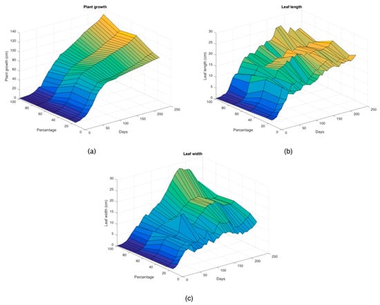
Figure 1.
Three-dimensional plots of experimental data for (a) plant growth, (b) leaf length and (c) leaf width.
The leaves under the treatments showed the typical characteristics of L. esculetum: compound, alternate pinnatisect, imparipinnate (with seven or nine leaflets on average), toothed or lobed leaflets and glandular hairs (Figure 2). Regarding their size, the leaf length in cm at the time of transplantation was statistically different, maintaining lengths of 2.4 cm (CNT+), 2.1 cm (T1), 2.0 cm (T2), 1.4 cm (T3), 1.0 cm (T4) and 0.4 cm (T5) among treatments, and after 56 days, leaf length did not show significant differences regarding CNT+ (Dunnett, α = 0.05). On the other hand, leaf width at transplantation measured 1.8 cm (CNT+), 1.4 cm (T1), 1.1 cm (T2), 0.9 cm (T3), 0.7 cm (T4) and 0.3 cm (T5), and at 245 days, the widest leaf corresponded to T5 and reached 18.1 cm on average, a measure significantly different from the leaves of the control (Dunnett, α = 0.05).
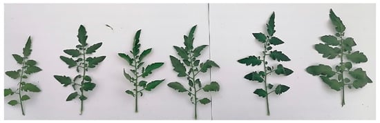
Figure 2.
The leaves of plants germinated with peat moss and degraded substrate under greenhouse conditions.
With these results, it was decided to apply the RSM and ANN to find the optimal concentration (best conditions) of degraded substrate to use in the germination of Lycopersicon esculetum that would allow seedlings capable of surviving in greenhouse conditions to be obtained and fruits intended for consumption to be generated, and thus demonstrate that it is possible to reduce the use of peat moss due to degraded substrate use in germination.
3.2. Response Surface Methodology
The RSM was developed, and the linear correlation graphs for plant growth and leaf width and length were plotted (Figure 3). The quadratic model showed the best fit for the three analyzed variables.
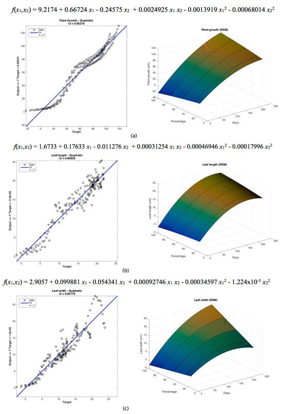
Figure 3.
RSM plots with quadratic model fit and linear correlation for (a) plant growth, (b) leaf length and (c) leaf width.
Equations (5)–(7) were obtained using RSM for fitting data on plant growth, leaf length and leaf width.
where x1 represents the number of days from the planting of seeds and x2 denotes the percentage of biodegraded substrate applied in the treatment.
f(x1,x2) = 9.2174 + 0.66724 x1 − 0.24575 x2 + 0.0024925 x1 x2 − 0.0013919 x12 − 0.00068014 x22
f(x1,x2) = 1.6733 + 0.17633 x1 − 0.011276 x2 + 0.00031254 x1 x2 − 0.00046946 x12 − 0.00017996 x22
f(x1,x2) = 2.9057 + 0.099881 x1 − 0.054341 x2 + 0.00092746 x1 x2 − 0.00034597 x12 − 1.224 × 10−5 x22
The ANOVA for the quadratic model of the response surface shows the influence of the two independent variables (x1 and x2) on the response variable. The ANOVA of the obtained model to represent the plant growth is shown in Table 4, with a Fisher value of 727.74 and a p-value much smaller than 0.0001.
The coefficient of determination r2 obtained from the comparison of experimental and forecasted data was 0.95218, i.e., more than 95% of the data were fitted properly (Figure 3a). The RMSE for this model was 7.53398, and the MAPE was 41.481212%. From this analysis, it can be confirmed that the response surface model can be used to forecast plant growth by knowing the applied treatment and the number of days from seed germination.
The regression analysis performed on this quadratic equation (Table 5) indicates that most of the variables were significant (p < 0.05), except for the square of the treatment variable, which had no significant impact on the equation.
The ANOVA for the quadratic equation modeling the response of plant growth is shown in Table 6. The Fisher value for this equation is 384.08, and its probability p-value is 5.42 × 10−92.
A value of 0.90939 was obtained as a coefficient of determination r2 from the comparison of the values gathered in the leaf length measurements and the values predicted by the RSM quadratic model. Therefore, it is shown that 90.939% of the data can be adequately modeled by this equation (Figure 3b). The RMSE obtained from the comparison between real and forecasted values was 1.85077, and the MAPE from actual and forecasted values was 21.426646%. The previous analysis demonstrates that this model can be used to forecast the leaf length by knowing the treatment type and the number of days from plant germination.
Furthermore, a regression analysis was performed (Table 7). The constant term, the linear term for the variable of the number of days, the interaction term of the variables of the number of days and treatment type, and the quadratic term of the number of days are all significant variables because their p-values were less than 0.05.
Finally, the ANOVA for the RSM quadratic model to forecast the leaf width is presented in Table 8, where the Fisher value (244.64) and the probability p-value (9.98 × 10−77) are shown.
A coefficient of determination r2 of 0.85775 was obtained from the comparison of the leaf width measurements and the values forecasted by the quadratic model. This r2 value indicates that 85.775% of the experimental data were modeled properly with the use of this quadratic equation (Figure 2c). The RMSE obtained was 2.14367, and the MAPE calculated was 28.881833%. This model can be applied to predict the leaf width, considering the treatment type and the number of days of plant germination, with a better precision than the equations presented above.
The regression analysis for this model shows that most of the terms are significant variables due to the p-value being less than 0.05 (Table 9). The only value that is not meaningful is the quadratic term of the variable for the treatment type, which has a p-value greater than 0.05.
3.3. Artificial Neural Network
Considering the coefficient of determination r2, the root mean square error (RMSE) and the mean absolute percentage error (MAPE), three ANNs with the best performance were obtained. The ANN with the best fitness for plant growth (r2 = 0.99979, RMSE = 1.2253, MAPE = 3.496504%) was composed of one input layer with two neurons, three hidden layers with two, five and three neurons, and an output layer with one neuron denoting plant growth (Figure 4a). The ANN linear correlation is shown in Figure 5a. The best conditions for germinating L. esculetum found by the ANN were the use of 100% biodegraded substrate and 245 days from the day the seeds were planted. Under these conditions, the maximum plant height obtained was 129.27 cm.
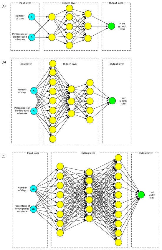
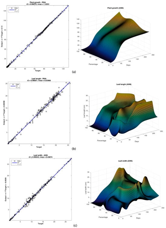
Figure 5.
ANN plots and linear correlation for (a) plant growth, (b) leaf length and (c) leaf width.
For calculating the leaf length, the ANN with the best performance was composed of the input layer with two neurons, and three hidden layers with nine, three and five neurons, respectively, and the output layer to denote the leaf length (Figure 4b). The linear correlation of this ANN is shown in Figure 5b. The determination coefficient for this ANN is r2 = 0.99001, RMSE = 0.63966 and MAPE = 4.650497%. This model predicts that the best conditions to maximize the leaf length are with a treatment considering 20% of biodegraded substrate in the L. esculetum germination and 192 days. The maximum leaf length calculated in these conditions is 26.48 cm.
Finally, the ANN with the best performance (r2 = 0.99343, RMSE = 0.49074, MAPE = 4.588313%) to calculate the leaf width (Figure 4c) had an input layer with two neurons, three hidden layers with eight, six and 10 neurons for each one, and an output layer with one neuron representing the leaf width. The linear correlation of this ANN is shown in Figure 5c. It predicts the maximum leaf width at 27.49 cm, considering 100% of biodegraded substrate and 183 days after the germination of tomato seeds.
To avoid overfitting, the ANNs were tested with a subset of data not used for training. The metrics of the ANN models are shown in Table 10.
Due to the small values of RMSE and MAPE and the r2 near 1, these metrics show the generalization of ANN models and, in consequence, the lack of overfitting.
Based on the ANN predictions, treatment number 5 (100% of biodegraded substrate applied in the germination) allowed the acquisition of seedlings with better phenological features than those that germinated with the application of commercial substrate (peat moss).
4. Discussion of Results
RSM is a set of mathematical and statistical techniques used to model and analyze problems in which the variable of interest is influenced by others [23]. In this work, the mathematical model obtained by RSM estimated the optimal value of an adequate amount of degraded substrate to germinate Lycopersicon esculetum and reduce the use of peat moss with viable plants for production. However, the ANN artificial intelligence method allowed the modeling of the growth behavior of tomato plants over 245 days. The results indicate that the optimal treatment for the germination of tomato seedlings is 100% degraded substrate. This model allows information whose behavior is complex, unpredictable, or chaotic (difficult to model by common mathematical models) to be processed and is highly tolerant to errors, which is why it behaves excellently when there are inaccuracies in the information [24].
The results of both methodologies were compared by calculating the coefficient of determination r2, the root mean square error (RMSE), and the mean absolute percentage error (MAPE) (Table 11) to determine which one provides the most accurate prediction and thus establish the best germination conditions for L. esculetum.
Both techniques offer a good data fit; however, the ANN provides the most reliable prediction, with an r2 higher than 0.99 for the three analyzed variables (plant growth, leaf length, and leaf width). On the other hand, the values of r2 obtained with RSM were lower. For RMSE and MAPE errors, the behavior was similar since errors obtained by ANN models were lower than those obtained by RSM models.
Therefore, the best condition for tomato germination is the use of 100% biodegraded substrate. The authors of [25] mention that the use of a correctly trained ANN model is more accurate in prediction than the RSM model. This work is a precedent for the implementation of ANNs in the prediction of the growth patterns of plants germinated with biodegraded substrate under greenhouse conditions. Other works have proposed the use of these methodologies to predict and estimate plant growth rates [26,27], conditions for obtaining fruits such as the loquat with desirable qualities [28], the germination of cereal seeds [29], in vitro germination and growth rates of Cannabis sativa L. [30], and the germination of seeds of Solanum lycopersicum L. [31]. The use of ANNs in agriculture has recently been used as a methodology that allows the evaluation of the cycle of any crop with the aim of generating optimized processes and thereby achieving greater productive efficiency. Therefore, its use in precision agriculture is suggested to replace classic modeling methods [32].
This work verifies that the use of ANNs in agriculture allows for the processing of experimental data and the proposing of the best conditions for tomato germination and the vegetative behavior of this crop in a greenhouse. Furthermore, the ANN confirms that the use of biodegraded substrate can be an alternative for the germination processes and in obtaining seedlings of various vegetables. These substrates show an ecological advantage since they present structural and nutritional changes that favor the development of plants, as well as improving interactions with the soil structure and the microorganisms present in the rhizosphere.
5. Conclusions
Bioinputs within organic agriculture must be efficient and increase crop yields, which is why it is necessary to evaluate their effect on crops. The use of mathematical models such as RSM and ANN is increasing within agriculture to predict and optimize processes. In this study, the use of the RSM and ANN models allowed us to predict the optimal conditions for tomato germination under greenhouse cultivation. The main contribution to the knowledge is the model generated by ANN and applied to the modeling and optimization of tomato plant behavior based on the treatment and the number of days from seed germination that presents a better fit than the RSM, indicating that plants obtained with biodegraded agave fiber substrate by P. djamor can generate plants with greater growth and development than those germinated with commercial peat moss. The implementation of these statistical models has practical applications in agriculture, allowing their use to be validated and thereby contributing to the generation of solutions aimed at the circular economy. Moreover, the application of the biodegraded substrate in tomato cultivation allows us to obtain plants with desirable phenological characteristics capable of competing with plants that come from the commercial substrate, so this material can be an alternative substrate that promotes the reduction of the use of commercial peat moss, since obtaining it leads to environmental damage in the ecosystems where it is found, unlike the reuse of waste from the fungal industry. As further work, this methodology will be applied to other biodegraded substrates to propose ecologically friendly alternatives to products that affect the environment and reduce the impact of climate change.
Author Contributions
Conceptualization, B.S.V.-d.-L. and J.Á.-C.; Funding acquisition, J.M.-M.; Investigation, B.S.V.-d.-L. and J.Á.-C.; Methodology, B.S.V.-d.-L., J.Á.-C., M.G.S.-D., E.M.H.-D. and J.M.-M.; Software, J.M.-M.; Validation, M.G.S.-D., E.M.H.-D. and J.M.-M.; Writing—original draft, B.S.V.-d.-L., J.Á.-C., M.G.S.-D., E.M.H.-D. and J.M.-M.; Writing—review and editing, J.Á.-C. and E.M.H.-D. All authors have read and agreed to the published version of the manuscript.
Funding
This study was partially supported by the National Council for Humanities, Science and Technology (CONAHCYT) with project number CB-2017-2018-A1-S-43008. Brianda Susana Velázquez De Lucio was supported by CONAHCYT grant number 732368.
Institutional Review Board Statement
Not applicable.
Data Availability Statement
The data presented in this study are available in this paper.
Acknowledgments
To the Universidad Politécnica de Pachuca for the facilities granted to the Academic Group “Manejo de sistemas agrobiotecnológicos Sustentables” for the development of the research project.
Conflicts of Interest
The authors declare that they have no known competing financial interest or personal relationships that could have appeared to influence the work reported in this paper.
References
- Maitra, S.; Brestic, M.; Bhadra, P.; Shankar, T.; Praharaj, S.; Palai, J.B.; Hossain, A. Bioinoculants Natural biological resources for sustainable plant production. Microorganisms 2021, 10, 51. [Google Scholar] [CrossRef] [PubMed]
- Leong, Y.K.; Ma, T.W.; Chang, J.S.; Yang, F.C. Recent advances and future directions on the valorization of spent mushroom substrate (SMS): A review. Bioresour Technol. 2022, 344, 126157. [Google Scholar] [CrossRef]
- Kraska, T.; Kleinschmidt, B.; Weinand, J.; Pude, R. Cascading use of Miscanthus as growing substrate in soilless cultivation of vegetables (tomatoes, cucumbers) and subsequent direct combustion. Sci Hortic. 2018, 235, 205–213. [Google Scholar] [CrossRef]
- Vieira, V.O.; Conceição, A.A.; Cunha, J.R.B.; Machado, A.E.V.; de Almeida, E.G.; Dias, E.S.; Alcantara, L.M.; Miller, R.N.G.; de Siqueira, F.G. A new circular economy approach for integrated production of tomatoes and mushrooms. Saudi J. Biol. Sci. 2022, 29, 2756–2765. [Google Scholar] [CrossRef] [PubMed]
- Vazquez-Cruz, M.A.; Luna-Rubio, R.; Contreras-Medina, L.M.; Torres-Pacheco, I.; Guevara-Gonzalez, R.G. Estimating the response of tomato (Solanum lycopersicum) leaf area to changes in climate and salicylic acid applications by means of artificial neural networks. Biosyst. Eng. 2012, 112, 319–327. [Google Scholar] [CrossRef]
- Zhang, R.H.; Duan, Z.-Q.; Li, Z.-G. Use of spent mushroom substrate as growing media for tomato and cucumber seedlings. Pedosphere 2012, 22, 333–342. [Google Scholar] [CrossRef]
- Wang, H.W.; Zhu, Y.X.; Xu, M.; Cai, X.Y.; Tian, F. Co-application of spent mushroom substrate and PGPR alleviates tomato continuous cropping obstacle by regulating soil microbial properties. Rhizosphere 2022, 23, 100563. [Google Scholar] [CrossRef]
- Asanza, W.R.; Olivo, B.M. Redes Neuronales Artificiales Aplicadas al Reconocimiento de Patrones (Artificial neural Networks Applied to Pattern Recognition); Editorial UTMACH: Machala, Ecuador, 2018. [Google Scholar]
- Zhang, J.; Lin, G.; Yin, X.; Zeng, J.; Wen, S.; Lan, Y. Application of artificial neural network (ANN) and response surface methodology (RSM) for modeling and optimization of the contact angle of rice leaf surfaces. Acta Physiol. Plant. 2020, 42, 51. [Google Scholar] [CrossRef]
- Xue, Z.; Fu, J.; Fu, Q.; Li, X.; Chen, Z. Modeling and Optimizing the Performance of Green Forage Maize Harvester Header Using a Combined Response Surface Methodology–Artificial Neural Network Approach. Agriculture 2023, 13, 1890. [Google Scholar] [CrossRef]
- Susanti, R.; Nofendra, R.; Zaini, Z.; bin Suhaimi, M.S.A.; Rusydi, M.I. The Use of Artificial Neural Networks in Agricultural Plants. Andalas J. Electr. Electron. Eng. Technol. 2022, 2, 62–68. [Google Scholar] [CrossRef]
- Vazquez-Cruz, M.; Jimenez-Garcia, S.; Luna-Rubio, R.; Contreras-Medina, L.; Vazquez-Barrios, E.; Mercado-Silva, E.; Torres-Pacheco, I.; Guevara-Gonzalez, R. Application of neural networks to estimate carotenoid content during ripening in tomato fruits (Solanum lycopersicum). Sci. Hortic. 2013, 162, 165–171. [Google Scholar] [CrossRef]
- Vargas, S.J.M.; López, C.I.L.; Rico, G.E. Redes neuronales artificiales aplicadas a mediciones de fitomonitoreo para simular fotosíntesis en jitomate bajo invernadero. Remexca 2012, 3, 747–756. [Google Scholar]
- Yang, Y.; Pan, Y.; Zhao, H.; Ji, A.; Shi, J.; Guo, P. Response surface optimization of cultivation conditions for yield of tomato (Lycopersicon esculentum Mill.) in greenhouses. J. Plant Nutr. 2018, 41, 210–220. [Google Scholar] [CrossRef]
- Cho, W.; Na, M.; Park, Y. Extraction of optimum condition of cultivation factors to improve tomato production using statistical regression analysis and response surface methodology. Adv. Sci. Lett. 2018, 24, 2084–2087. [Google Scholar] [CrossRef]
- Velázquez-De Lucio, B.S.; Téllez-Jurado, A.; Hernández-Domínguez, E.M.; Tovar-Jiménez, X.; Castillo-Ortega, L.S.; Mercado-Flores, Y.; Álvarez-Cervantes, J. Evaluation of bagasse Agave salmiana as a substrate for the cultivation of Pleurotus djamor. Rev. Mex. Ing. Química 2022, 21, Bio2735. [Google Scholar] [CrossRef]
- Medina, E.; Paredes, C.; Pérez-Murcia, M.D.; Bustamante, M.A.; Moral, R. Spent mushroom substrates as component of growing media for germination and growth of horticultural plants. Bioresour. Technol. 2009, 100, 4227–4232. [Google Scholar] [CrossRef]
- Aggarwal, C.C. Neural Networks and Deep Learning; Springer: Berlin/Heidelberg, Germany, 2018; Volume 10, p. 3. [Google Scholar]
- Zhang, Z.; Feng, Q.; Huang, J.; Guo, Y.; Xu, J.; Wang, J. A local search algorithm for k-means with outliers. Neurocomputing 2021, 450, 230–241. [Google Scholar] [CrossRef]
- Hagan, M.T.; Demuth, H.B.; Beale, M.H.; De Jesus, O. Neural Network Design, 2nd ed.; Oklahoma State University: Stillwater, OK, USA, 2014; Available online: http://hagan.okstate.edu/NNDesign.pdf (accessed on 6 October 2023).
- Geyikçi, F.; Kılıç, E.; Çoruh, S.; Elevli, S. Modelling of lead adsorption from industrial sludge leachate on red mud by using RSM and ANN. Chem. Eng. J. 2012, 183, 53–59. [Google Scholar] [CrossRef]
- López, M.L.M. Manual Técnico del Cultivo del Tomate: Solanum lycopersicum; Instituto Nacional de Innovación y Transferencia en Tecnología Agropecuaria (INTA): Ciudad de México, México, 2017.
- Askari, M.; Abbaspour-Gilandeh, Y.; Taghinezhad, E.; El Shal, A.M.; Hegazy, R.; Okasha, M. Applying the Response Surface Methodology (RSM) Approach to Predict the Tractive Performance of an Agricultural Tractor during Semi-Deep Tillage. Agriculture 2021, 11, 1043. [Google Scholar] [CrossRef]
- Escamilla, G.A.; Soto, Z.G.M.; Toledano, A.M.; Rivas, E.; Gastélum, B.A. Applications of artificial neural networks in greenhouse technology and overview for smart agriculture development. Appl. Sci. 2020, 10, 3835. [Google Scholar] [CrossRef]
- Maran, J.P.; Sivakumar, V.; Thirugnanasambandham, K.; Sridhar, R. Artificial neural network and response surface methodology modeling in mass transfer parameters predictions during osmotic dehydration of Carica papaya L. alexandria. Eng. J. 2013, 52, 507–516. [Google Scholar] [CrossRef]
- Pohan, S.; Warsito, B.; Suryono, S. Backpropagation artificial neural network for prediction plant seedling growth. J. Phys. Conf. Ser. 2020, 1524, 012147. [Google Scholar] [CrossRef]
- Gall, G.E.C.; Pereira, T.D.; Jordan, A.; Meroz, Y. Fast estimation of plant growth dynamics using deep neural networks. Plant Methods 2022, 18, 21. [Google Scholar] [CrossRef] [PubMed]
- Huang, X.; Wang, H.; Qu, S.; Luo, W.; Gao, Z. Using artificial neural network in predicting the key fruit quality of loquat. Food Sci. Nutr. 2021, 9, 1780–1791. [Google Scholar] [CrossRef]
- Genze, N.; Bharti, R.; Grieb, M.; Schultheiss, S.J.; Grimm, D.G. Accurate machine learning-based germination detection, prediction and quality assessment of three grain crops. Plant Methods 2020, 16, 157. [Google Scholar] [CrossRef]
- Aasim, M.; Katırcı, R.; Akgur, O.; Yildirim, B.; Mustafa, Z.; Nadeem, M.A.; Baloch, F.S.; Karakoy, T.; Yılmaz, G. Machine learning (ML) algorithms and artificial neural network for optimizing in vitro germination and growth indices of industrial hemp (Cannabis sativa L.). Ind. Crops Prod. 2022, 181, 114801. [Google Scholar] [CrossRef]
- Škrubej, U.; Rozman, Č.; Stajnko, D. The accuracy of the germination rate of seeds based on image processing and artificial neural networks. Agricultura 2015, 12, 19–24. [Google Scholar] [CrossRef]
- Kujawa, S.; Niedbała, G. Artificial Neural Networks in Agriculture. Agriculture 2021, 11, 497. [Google Scholar] [CrossRef]
Disclaimer/Publisher’s Note: The statements, opinions and data contained in all publications are solely those of the individual author(s) and contributor(s) and not of MDPI and/or the editor(s). MDPI and/or the editor(s) disclaim responsibility for any injury to people or property resulting from any ideas, methods, instructions or products referred to in the content. |
© 2023 by the authors. Licensee MDPI, Basel, Switzerland. This article is an open access article distributed under the terms and conditions of the Creative Commons Attribution (CC BY) license (https://creativecommons.org/licenses/by/4.0/).