Live Pig-Weight Learning and Prediction Method Based on a Multilayer RBF Network

Abstract

The live weight of pigs has always been an important reference index for growth monitoring and the health status of breeding pigs. An accurate weight acquisition of breeding pigs is the key to guide the scientific feeding of breeding pigs and improve economic benefits. Compared with the traditional contact measurement method, the non-contact weighing method of live pigs can greatly reduce human–pig contact and measurement errors. In this paper, a deep neural network is constructed which can automatically and accurately predict the weight of live pigs by measuring multiple body parameters. Because of the good generalization ability of the radial basis function (RBF) neural network and the better fitting ability of multilayer network than the traditional single-layer network, this paper introduces a full-connection model in the middle layer, connects multiple RBF layers, builds a multilayer RBF network, and invents the automatic learning method of pig weight based on the network. In this method, the body length, body height, body width, and five other body parameters are input, after normalization, into the multilayer RBF network model for training, and resultingly the network gives a predicted weight. Among our 4721 live pigs, there are 2452 sows and 2269 boars, among which 2000 samples of sows are randomly selected as training sets and 452 samples as test sets; 1930 samples of boars are taken as training sets and 339 samples as test sets. The test shows that the performance of the network structure is as follows: R2 is 0.63, MAE is 1.85, RMSE is 5.74, and MAPE is 1.68.

1. Introduction

Live weight is an important index of pigs, and obtaining the weight of pigs quickly and accurately can evaluate the growth and health status of pigs immediately and detect the feed absorption rate of pigs accordingly. It can also help in raising pigs with different nutritional status separately, to achieve the maximum utilization rate of feed and the best growth control. Similarly to Ahmad Alsahaf et al. [1], who used random forest algorithms to predict the age and weight of pigs, measuring the weight of live pigs automatically and accurately is one of the research focuses of intelligent agriculture at present. Traditional pig weight detection often requires direct contact with pigs, and pigs need to be moved to weighing equipment, such as electronic scales. The whole process is not only time-consuming but also laborious, and the error of manual measurement is large, requiring human and animal contact, which easily causes the spread of diseases. Sometimes it is necessary to use sedatives and other drugs to assist, which brings great pressure to pigs, affects daily activities such as eating and mating, and even causes the sudden death of pigs, resulting in great economic losses.

Recently, a variety of methods have been proposed to evaluate the body weight of live pigs, which can be divided into two categories, namely direct measurement and indirect measurement. Direct measurements usually use scales to weigh live pigs in contact. Sharp et al. [2] developed a self-weighing scale, which can automatically estimate the weight of the forelegs or hind legs of pigs in daily activities such as eating. This technology can determine the weight of live pigs without affecting their daily activities, but it requires establishing an electronic weighing platform in front of the feeder, and a pig needs to be evaluated by repeatedly obtaining a large amount of data, which is easily affected by bad data.

The indirect measurement method mainly obtains the image data of live pigs according to computational vision, and then evaluates the weight of live pigs according to relevant algorithms. According to the principle of animal feeding, there is a significant correlation between the size and weight of animals, so the indirect measurement method, based on computer vision, has become the mainstream way to weigh live pigs. This kind of method first captures the image of live pigs, and then extracts the features of live pigs in the image to predict the weight of pigs directly and accurately. For example, Brandl et al. [3] set out to determine the weight of live pigs from dimensions measured by an image analysis system. Wang et al. [4] extracted physical and morphological features including the back area and center width from the acquired live pig image by processing the captured image, and applied the proposed mathematical model to predict the live pig weight. However, in this method, each live pig needs to be photographed for about one minute, and the movement of the live pig leads to the continuous change of projection shape, which leads to errors. Therefore, it is necessary to manually check and select images of the pig’s body and head in a standing state to ensure consistency and accuracy. Tscharke et al. [5] installed cameras on the top and side of live pigs, using multiple cameras to obtain the back area and body height of live pigs. At the same time, to reduce the number of cameras, a mirror was installed on top of the pigs at a 45-degree angle to capture the back area and height information of pigs. However, the cameras were easily polluted by dirt, and the measured live pigs were easily blocked by other live pigs. Song et al. [6] used an automatic measurement system to extract the morphological features of cows in a 3D vision system, used a multiple linear regression model to predict weight, and used an exhaustive feature selection algorithm to establish an intermediate model. Kashiha et al. [7], captured the top image of live pigs, and separated the head and neck from the body in the image to maximize the correlation with body weight. The ellipse fitting algorithm of generalized Hough transform was adopted to calculate the area occupied by pigs in the ellipse, and the dynamic model was used to estimate the weight of pigs, but proper lighting was needed. White et al. [8] used the visual image analysis system to obtain the area and length measurements of 11 live pigs, such as the width of the widest shoulder, the contraction between shoulder and trunk, and the total plane area of the body, and designed a regression model to estimate the weight of live pigs. Minagawa et al. [9] used a technology similar to structured light to measure the height of live pigs, fixed the camera on the ceiling above the drinking fountain, and established a mathematical model to predict the weight of live pigs by using the geometric relationship between pixel difference and height. Minagawa [10] took stereo photography of live pigs, estimated the surface area of live pigs by stereophotogrammetry with two non-measurement cameras, set up 28 control marks to estimate that the body was formed by adjacent cross-sections and assumed to be conical, and measured the area by calculating the number of cross-sections of 1 mm square area for weight estimation, but the limb shape was complex and the accuracy was low. Li et al. [11] used infrared depth images to obtain row vectors and vectors measured by pig volume for weight prediction, but the posture of live pigs still had a significant impact on weight estimation. In the same year, Kongsro [12] presented a prototype for pig weighing based on Microsoft Kinect camera technology utilizing infrared depth map images. Shi et al. [13] used binocular stereo vision system to obtain the image of live pigs, and used depth information to eliminate background interference. According to the regression results of the least square method, the relevant parameters for predicting the weight function of live pigs were calculated, but this method was greatly affected by image quality. Pezzuolo et al. [14] used the Microsoft Kinect v1 (Microsoft, Redmond, America) depth camera for fast, non-contact measurements of pig body dimensions such as heart circumference, length, and height, and developed two models (linear and nonlinear) and applied them to the Kinect and Measure data manually. Finally, a nonlinear model was used to exploit the full performance of the Kinect depth camera, reducing the standard error of the estimate.

With the rise of deep learning, many studies have applied deep learning to the weight estimation of live pigs. Kaewtapee et al. [15] obtained the top images of pigs, binarized and segmented the pig body for morphological operation, calculated the ratio of live pig pixels to total area, and established the estimation model of live pig-weight by regression analysis and artificial neural network (ANN). In addition, Tasdemir et al. [16], through multiangle analysis of cow images obtained in a synchronous 3D camera environment, determined the cow physique and constructed ANN to estimate the live weight. Bhatt et al. [17] used SegNet to segment sheep from the background, and output the segmented results to estimate the live weight by ANN, but this method needs a 3D image and is easily affected by the background. Spoliansky et al. [18] using the Kinect camera and its automatic BCS system, put forward an image-processing algorithm for live cattle, which can effectively estimate the live weight by polynomial regression, and this method can effectively avoid background influence. Haile-Mariam et al. [19] predicted weights by fitting the multiple regression model. Jensen et al. [20] converted the obtained image of live pigs into gray-scale image, and improved the contrast, which was used in a convolution neural network (CNN) to predict the weight of live pigs. Cang et al. [21] constructed a network based on the Faster-RCNN network and regression branch, and estimated that weight of live pigs by taking the back of the captured live pig as the input of the network. Huma et al. [22] used the body and testicle measurements of Balochi sheep to construct a random forest model to predict the live weight. Wang et al. [23] extracted features such as area, convex surface area, circumference, and eccentricity from captured live pig images, and put them into the constructed three-layer ANN to estimate the weight of live pigs. However, there are high requirements for captured live pig images, and the threshold set during the binarization operation is related to the surrounding light. He et al. [24] selected LASSO regression and two machine learning algorithms (random forest and long short-term memory network) to forecast the body weight of pigs and investigated the usefulness of feeding behavior data in predicting the body weight of pigs at the finishing stage.

Although many live pig-weight assessment methods have been proposed, most of them are influenced by the posture and exercise of live pigs. In the direct measurement method, it is difficult to solve the downward force caused by the movement of live pigs, except the weight. In the indirect measurement method, the current methods need to get the two-dimensional area of live pigs. The acquisition of this parameter requires higher accuracy for the captured images, and the pigs need to be in a relatively fixed position, which is extremely vulnerable to the influence of the posture of live pigs. According to the principle of animal husbandry, there is a potential relationship between the body parameter and the weight of pigs. After the pig breed is determined, the automatic estimation of the weight of pigs can be realized by constructing a deduction model of the body parameter and the weight. At the same time, if there is only a need to obtain several one-dimensional physical characteristics of live pigs, such as body height, length, and circumferences, then the image requirements for capturing pigs will be much lower, as the captured image will have greater robustness. Therefore, this paper constructs a multilayer RBF network deep learning model, which only takes several one-dimensional body characteristics of live pigs as network inputs, and obtains the nonlinear relationship between body parameters and weight data by learning and training a large number of body parameters and weight data, and then realizes the accurate calculation of live pig weight.

2. Material and Methods

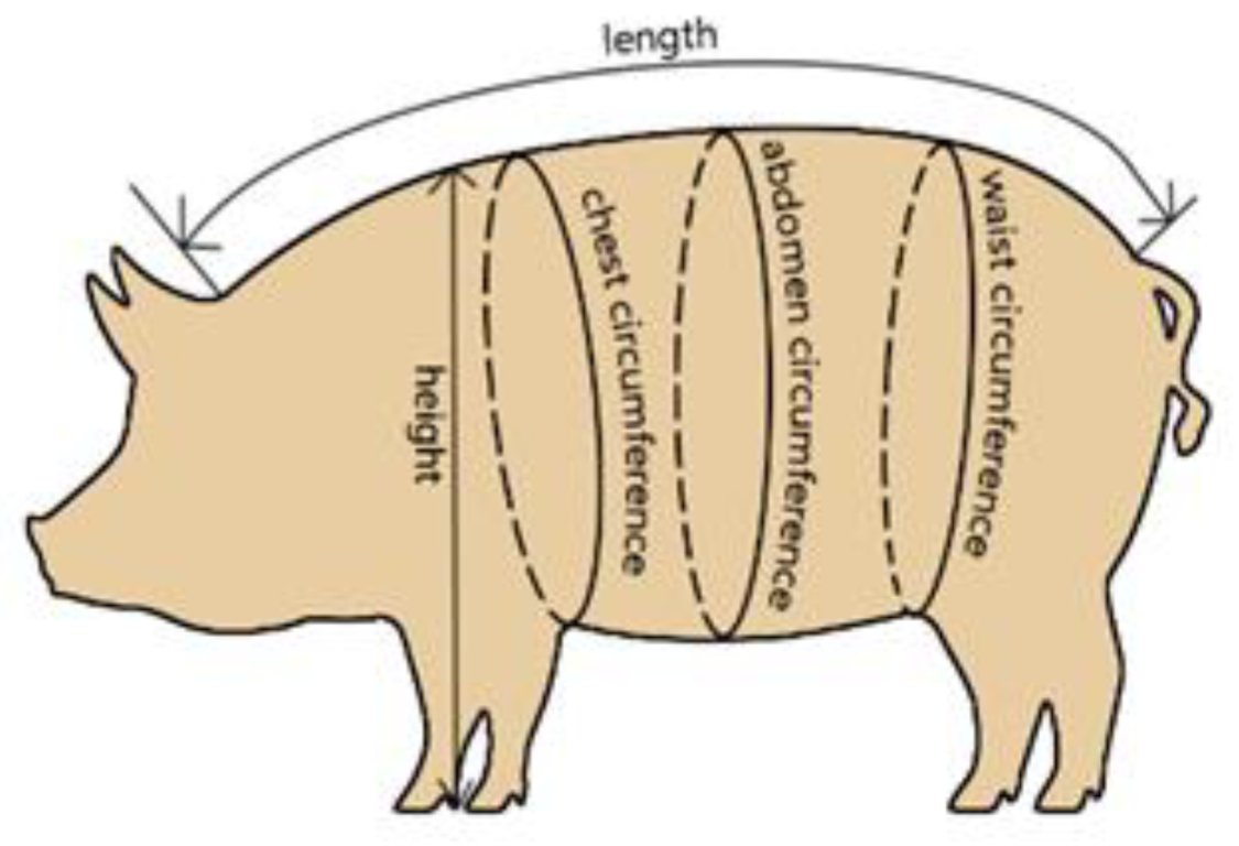
2.1. Data

The data is from a large, listed company in China, collected from 2016 to 2020, in Guangdong Province, China, and includes 4721 American Duroc boars and sows. Walugembe et al. [25] have proved that four body measurements (body length, heart girth, height, and body width) were strongly predictive (R2 = 0.92) of live body weight for the ≥40 kg pigs. Other research [26] has reported a strong correlation between live body weight and heart girth in finishing pigs. In this paper, each live pig was measured for its height, length, chest circumference, abdomen circumference, and waist circumference, and the age of each live pig was limited to 150–190 days. The surveyor uses a tape measure to measure the parameters of the live pig. The live pig is fixed in a special cage to keep its body straight. The length is measured from the neck to the tail. The measurement of chest circumference is the circumference of body to the rear of the front leg. The abdomen circumference is the abdominal circumference between the front leg and the rear leg. The waist circumference is the circumference of body to the front of the rear leg. The height is the length from the bottom of the front leg to the neck when the live pig is upright. The measurement standard of live pigs is shown in Figure 1, and the unit is centimeters. The measuring range of body parameter is set according to the suggestion of animal husbandry experts. Specifically, the length is from the middle of the head and ears to the root of the tail. The height is the highest point from the bottom of the front leg to the shoulder and neck of the pig. The chest circumference is the circumference of the pigs behind the front legs. The abdomen circumference is the circumference of pigs at the midpoint of the front legs and hind legs. The waist circumference is the circumference of a pig in front of its hind legs. Data measurement is obtained through manual measurement by specialized technical personnel using uniform standards, as shown in

Table 1. Body parameter data for the five sample pigs.

Serial Number	Body Length (cm)	Height (cm)	Chest Circumference (cm)	Abdomen Circumference (cm)	Waist Circumference (cm)	Body Weight (kg)
1	121	67	105	115	103	117.5
2	120	69	107	118	105	113.7
3	117	64	103	111	104	105.6
4	125	69	108	120	107	120.0
5	126	65	111	123	110	120.3

.

2.2. Data Preprocessing

Data normalization processing is a basic work of network learning. Different evaluation indicators often have different dimensions, and the values may vary greatly. Failure to deal with them may affect the results of network training.

We used MinMax normalization, PolynomialFeatures algorithm, MaxAbs normalization, FunctionTransformer algorithm, and Z-score normalization. Z-score normalization was chosen because it is applicable to numerical data, is not affected by the magnitude of data, and exhibited the best performance. The Z-score is defined as

$$y=\frac{x-\mu }{\sigma }$$

(1)

where μ is the mean value of the original data, and σ is the standard deviation of the original data, which is currently the most widely used data standardization method. The data above the mean value will obtain a positive standardized score, and vice versa.

2.3. RBF Network Structure

Radial basis function (RBF) is a kind of feedforward neural network which uses radial basis function as activation function, and then makes a linear combination of hidden neurons. In theory, the RBF network has proved that it can approach any nonlinear function, and can deal with regularity that is difficult to analyze in the system (Maruyama et al., 1992) [27]. It has good generalization ability and a fast learning-convergence speed. Compared with the BP neural network (for BP neural network is a global approximation network), one or more parameters in its network will affect the output; for each input, the weights on the network need to be adjusted, which leads to its slow learning speed. In the fully connected neural network, the S-type function will generate displacement, the weight will change the slope of displacement, and the bias value will change the position of displacement. The RBF network model adopts a Gaussian radial basis function, also called the Gaussian kernel function, in which locality is the key characteristic. Each Gaussian kernel will only have a few weights in a local area of input space, which will affect input data. Therefore, only the corresponding parameters of input data need to be adjusted each time, and the learning speed is fast. If the RBF layer has enough uniformly distributed Gaussian kernel functions, we can, in theory, approach any interested function.

The radial basis function used in this paper is Gaussian kernel function, which is defined as:

$$\phi \left(X\right)=e^{-\frac{1}{2{\sigma }^2}{\left|\left|x_p-c_i\right|\right|}^2}$$

(2)

where $c_i$ denotes the i-th center point, $x_p$ is the p-th data, $\left|\left|x_p-c_i\right|\right|$ is the Euclidean distance from sample $x_i$ to the center $c_i$, $\sigma$ is a variable that can be set, which controls the radial basis function around the width of the corresponding center point, the shape of the gaussian function, and the range of the basis function. As shown in Figure 2a, the red point is the center point $c$ of the Gaussian kernel function and the input data in the range of the blue to the Gaussian kernel function of the corresponding region. As shown in Figure 2a,b, if the input data move too far from the Euclidean distance of the center point of the Gaussian kernel function, the output of the corresponding neuron will be close to zero. However, as the distance increases, $\phi \left(X\right)$ will decrease sharply, which means in learning, the data far from the center point will not affect the update of the center point; in prediction, the center point will not affect the data far from it. These centers constitute the hidden layer space, so that the input vector can be directly mapped to the hidden layer space, rather than connected by the weight. Therefore, for the RBF network, the activation response of each transmission data is local only in a small area of the input space. $\sigma$ controls the size of the red region, which creates the RBF network local fitting characteristics.

When the center point is determined, the corresponding mapping relationship is determined, which can map the vector from the low dimension to the high dimension. The input data will be expanded in the form of the polynomial kernel and mapped from low dimension to high dimension.

In this paper, the traditional single-layer RBF network is improved to a multilayer RBF network, in which the full connection layer is inserted for connection. According to the previous paragraph, the single-layer RBF network structure has excellent local fitting ability; the multilayer RBF network can further improve the function-fitting ability of the RBF network. The principle is that the second-layer RBF network is used to fit the fitting residual function of the first layer, then the third-layer RBF network is used to fit the fitting residual network of the second-layer RBF network, and the latter layer is used to fit the previous layer network, in turn, so that a multilayer RBF network with high fitting ability is obtained.

However, if the distribution of the center points in the hidden layer space is not uniform enough, and most of the activation spaces corresponding to the center points overlap, then the fitting of the network will be greatly reduced. Therefore, the RBF network in this paper will learn the input training set data and adjust the position of the center point by the gradient descent method.

Finally, with the weight of each layer, the position of the center point and the width of the kernel function are learned and adjusted by the gradient descent method and we can obtain a multilayer RBF network model with a high fitting ability.

2.4. The Model of Deep Learning Network Framework in This Paper

Figure 3 shows the flow chart. The multilayer RBF network structure of this paper is shown in Figure 4. The Gaussian kernel function of the first layer is expanded and described in the figure. Firstly, the input data is mapped from low dimension to high dimension, and the Euclidean distance between the data mapped to high dimension and each central point is calculated in turn, that is $d_i=\left|\left|x_i-c_i\right|\right|$. $x_i$ is the input data mapped on the ith RBF kernel, and according to the shape of the kernel function controlled by $\sigma$, this is $m_i=\sigma .\ast \left|\left|x_i-c_i\right|\right|$. $m_i$ represents the shape of the kernel function on the i-th RBF kernel, which controls the width of the kernel function around the center point, the shape of the Gaussian function, and the range of the kernel function, then through the gaussian kernel function, $g_i=e^{-\frac{1}{2{\sigma }^2}{\left|\left|x_i-c_i\right|\right|}^2}$. $g_i$ is the output value of the i-th Gaussian kernel function, and the response values of all center points under the kernel function are output in turn. If the Euclidean distance between some center points of the kernel function is too large, it can be concluded from the characteristics of the Gaussian kernel function that the output value of the kernel function approaches zero. Then, the Gaussian kernel function has no effect on the data, and the data will not adjust the Gaussian kernel function in the back propagation, so that the network structure can learn quickly and has strong local fitting ability. Then, connected with the fully connected layer, where $t_j^k$ is the output value of the j-th neuron in the kth layer of the fully connected layer, $w_j^k$ represents the weight of the j-th fully connected neuron in the k-th layer, and $b^k$ represents the bias of the k-th layer of the fully connected layer, and then connects to the next RBF layer until the weight estimation value is finally output. In this way, each layer of RBF is connected together through the full connection layer, which constitutes the multilayer RBF network used in this paper.

In this paper, we tested and verified the RBF network structure from single layer to ten layers. We divided the data into a training set (70%) and a test set (30%), and set up a verification set (20% of training set) to verify the hyperparameters. The GridSearchCV algorithm from the SKlearn library [28] was used for RBF network structure with different layers each time to automate the process of obtaining the best combination of hyperparameters. In the training process, we used the dropout algorithm to restrain the overfitting. To obtain a more accurate network model, we used cross-validation algorithms and an early stopping technique. Finally, the three-layer RBF network structure has the best performance. Fewer RBF layers show a weak fitting ability, and more RBF layers will produce overfitting before training is completed. The result will be shown in the next section with other machine learning algorithms.

2.5. BP network and Machine Learning Algorithms

In this paper, the traditional fully connected neural network (BP network) and machine learning algorithms were also used for experiments. As well as the BP network, we mainly focus on the following regression algorithms: random forest (RandomForestRegressor), extra trees (ExtraTreesRegressor), k-nearest neighbours (KNeighborsRegressor), linear regression (LinearRegression), gradient boosting (GradientBoostingRegressor), Bayesian ridge (BayesianRidge), scaled gradient boosting (XGBRegressor) [29], and gradient boosting (CatBoostRegressor) [30].

As same as the RBF network, we used GridSearchCV to automate the process of obtaining the best combination of hyperparameters. The dropout algorithm, cross-validation algorithms and early stopping technique were used during the training process.

3. Result

The experiment was completed by a computer with 16 G memory, an i7 processor, and an RTX2060 graphics card under the Windows operating system. After GPU acceleration was turned on, the network training was completed after 60 iterations, which only took about 4 min. Experiments were carried out on boars, sows, and mixture of boars and sows, with five experiments in each group. The BP network and machine learning group mainly focus on mixture of boars and sows.

The distribution of data on the growth date and weight of all pigs that we used was input to the above two networks is shown in Figure 5. The age of boars and sows was mainly between 150 and 190 days. The weight of boars was generally higher than that of sows, but the weight distribution of boars was more dispersed than that of sows.

To find the optimal response, we used an exhaustive search method to test various combinations of hyperparameters. The results of various evaluation measures used to evaluate model performance on the training and test datasets is shown in

Table 2. Performance comparison of all models in R², RMSE, MAE, and MAPE.

Algorithm	On Training Dataset				On Testing Dataset
	R2	MAE	RMSE	MAPE	R2	MAE	RMSE	MAPE
RandomForestRegressor	0.59	2.01	6.44	1.82	0.38	2.05	6.55	1.85
ExtraTreesRegressor	0.65	1.95	5.82	1.76	0.43	1.96	5.99	1.78
KNeighborsRegressor	0.71	1.83	5.25	1.65	0.48	1.99	6.27	1.81
GradientBoostingRegressor	0.69	1.88	5.67	1.71	0.53	1.92	5.76	1.73
XGBRegressor	0.74	1.77	4.89	1.59	0.53	1.91	5.97	1.73
CatBoostRegressor	0.70	1.88	5.61	1.70	0.54	1.89	5.67	1.71
BayesianRidge	0.54	2.18	7.66	1.99	0.44	2.24	7.75	2.02
BP Network	0.52	2.10	6.58	1.91	0.43	2.26	8.07	2.03
Multilayer RBF network	0.72	1.68	5.03	1.53	0.63	1.85	5.74	1.68

R²: Coefficient of determination, MAE: mean absolute error, RMSE: root mean square error, MAPE: mean absolute percentage error.

. We tested and verified single-layer to ten-layer BP networks, and the three-layer BP network structure had the best performance with a consistent R² of 0.52 on the training dataset and 0.43 on the test dataset. In machine learning, we tested and verified RandomForestRegressor, ExtraTreesRegressor, KNeighborsRegressor, GradientBoostingRegressor, XGBRegressor, CatBoostRegressor, and BayesianRidge. Among them, CatBoostRegressor algorithm had the smallest MAE of 1.89 and MAPE of 1.71 on the test dataset. As shown in Table 2, in all algorithms, the multilayer RBF network had the smallest MAE of 1.85 and MAPE of 1.6 on the test dataset, and the consistent R² of 0.63 shows that the multilayer RBF network has the best fitting ability.

We used the 10-fold cross-validation algorithm to verify the performance indicators of the multilayer RBF network structure. For 10 iterations, the evaluation metrics were almost unchanged, indicating the prediction stability of the multilayer RBF network structure. At the same time, it can be concluded that the fitting ability of the multilayer RBF network structure is stronger than others. The result is shown in

Table 3. Results of 10-fold cross-validation. SD (×10⁻⁴) is the standard deviation.

Algorithm	R2		MAE		RMSE		MAPE
	Mean	SD	Mean	SD	Mean	SD	Mean	SD
Multilayer RBF network	0.66	0.037	1.95	0.012	6.15	0.069	1.71	0.011

.

For more detailed information, we also divided boars and sows into groups. Figure 6 describes the prediction results of the weight of Duroc boars, sows, and mixture of boars and sows after training by the RBF network. The x-axis shows the actual weight of live pigs and the y-axis shows the predicted weight of live pigs by the neural network. Each blue dot represents one pig, and the red line represents the perfect weight prediction, which means the predicted weight equals to the actual weight. Therefore, the closer to the red line, the more perfect the prediction result is. In the multilayer RBF network, sow weight (the first picture in Figure 6) is better than boar weight (the second image in Figure 6), and boar weight prediction is better than mixed sow weight (the third picture in Figure 6). As shown in

Table 4. Prediction performance of multilayer RBF networks on different gender.

Breed and Gender	On Training Dataset				On Testing Dataset
	R2	MAE	RMSE	MAPE	R2	MAE	RMSE	MAPE
Duroc boar	0.89	1.08	2.08	0.95	0.85	1.40	3.48	1.23
Duroc sow	0.84	1.05	2.02	0.96	0.79	1.20	2.77	1.10
Duroc boars and sows mixed	0.72	1.68	5.03	1.53	0.63	1.85	5.74	1.68

, the sow weight prediction has the smallest MAE of 1.20 and MAPE of 1.10 on the test dataset, and the consistent R² is 0.79. The boar weight predictions’ MAE, MAPE, and R² are 1.40, 1.23, and 0.85, respectively.

4. Discussion

In predictions of body parameter and weight, data features are not global, so the Gaussian kernel of RBF neural network can learn the local features of data, respectively, therefore when the local characteristics of the data are inconsistent, the multilayer RBF network structure can still have a strong fitting ability. For example, many live pigs with the same weight but different body parameters have great weight errors predicted by the other model, because the data cannot be fitted separately.

It can be concluded from Figure 6 and Table 4 that the data distribution of the sow’s weight and age is more uniform, and the RBF network can extract local features well, while the data distribution of the boar’s weight and age deviates from the average value and is scattered. In fitting local features of data deviating from the average value, the RBF network has less local data and a poor local-fitting effect, so the prediction effect for the sow is better than that of the boar in the prediction result of RBF network. However, after mixing, the local characteristics of sows and boars are different, so that there are different characteristics in the similar body parameter and weight data, which leads to the reduction of the local fitting effect of RBF network, and the effect is worse than that measured for sows and boars individually. Table 2 also shows that the absolute error and relative error of sows are better than those of boars.

In a word, according to the above experiments, the RBF network can fit the weight prediction well. At the same time, it greatly reduces the amount of calculation by using the kernel center point and constructing a multilayer RBF network layer with a full connection layer, which not only improves the accuracy of weight prediction, but also improves the efficiency of network prediction, which reduces the requirements for equipment and has a good effect on live weight prediction.

5. Conclusions

Most live pig-weight prediction based on computer vision neural networks is based on two-dimensional area parameters of live pigs. However, in agricultural production, harsh environment, illumination, and the changing posture of live pigs will lead to abnormal and unstable prediction systems. In this paper, the multilayer radial basis function network is used to predict the body weight through one-dimensional body parameters which are relatively measured and not easy to change with the posture change of live pigs. Compared with the machine learning algorithm, the multilayer RBF network structure has higher accuracy, and the tenfold cross-validation method also confirms the stability of the network structure in the test set and training set. At the same time, due to the reduction of measurement requirements, the requirements of required equipment are also reduced, which can effectively reduce its cost in agricultural production. In the follow-up work, we can use the computer vision system to measure the one-dimensional body parameters of live pigs, and try to reduce the number of body parameters and find the most relevant body parameter for weight prediction.

References

1. Alsahaf, A.; Azzopardi, G.; Ducro, B.; Hanenberg, E.; Veerkamp, R.F.; Petkov, N. Prediction of Slaughter Age in Pigs and Assessment of the Predictive Value of Phenotypic and Genetic Information Using Random Forest. J. Anim. Sci. 2018, 96, 4935–4943. [Google Scholar] [CrossRef]
2. Sharp, J.R.; Turner, M.J.B. Automatic Weight Monitoring of Pigs—Part II: Analysis of Results From Trial Work of Mk II In-Pen Pig Weigher; National Institute of Agricultural Engineering Divisional Note DN: Silsoe, UK, 1985; p. 1267. [Google Scholar]
3. Brandl, N.; Jørgensen, E. Determination of Live Weight of Pigs from Dimensions Measured Using Image Analysis. Comput. Electron. Agric. 1996, 15, 57–72. [Google Scholar] [CrossRef]
4. Wang, Y.; Yang, W.; Winter, P.; Walker, L.T. Non-contact sensing of hog weights by machine vision. Appl. Eng. Agric. 2006, 22, 577–582. [Google Scholar] [CrossRef]
5. Tscharke, M.; Banhazi, T.M. Growth Recorded Automatically and Continuously by a Machine Vision System for Finisher Pigs. Aust. J. Multi-Discip. Eng. 2013, 10, 70–80. [Google Scholar] [CrossRef] [Green Version]
6. Song, X.; Bokkers, E.A.M.; van der Tol, P.P.J.; Groot Koerkamp, P.W.G.; van Mourik, S. Automated Body Weight Prediction of Dairy Cows Using 3-Dimensional Vision. J. Dairy Sci. 2018, 101, 4448–4459. [Google Scholar] [CrossRef] [PubMed] [Green Version]
7. Kashiha, M.; Bahr, C.; Ott, S.; Moons, C.P.H.; Niewold, T.A.; Ödberg, F.O.; Berckmans, D. Weight Estimation of Pigs Using Top-View Image Processing. In Image Analysis and Recognition; Campilho, A., Kamel, M., Eds.; Lecture Notes in Computer Science; Springer International Publishing: Cham, Switzerland, 2014; Volume 8814, pp. 496–503. [Google Scholar] [CrossRef]
8. White, R.P.; Schofield, C.P.; Green, D.M.; Parsons, D.J.; Whittemore, C.T. The Effectiveness of a Visual Image Analysis (VIA) System for Monitoring the Performance of Growing/Finishing Pigs. Anim. Sci. 2004, 78, 409–418. [Google Scholar] [CrossRef] [Green Version]
9. Minagawa, H.; Murakami, T. A hands-off method to estimate pig weight by light projection and image analysis. In Livestock Environment VI, Proceedings of the 6th International Symposium 2001, Louisville, KY, USA, 21–23 May 2001; American Society of Agricultural and Biological Engineers: St. Joseph, MI, USA, 2001. [Google Scholar] [CrossRef]
10. Minagawa, H. Stereo Photogrammetric Errors in Determining the Surface Area of a Small Pig Model with Non-Metric Cameras. J. Agric. Meteorol. 1995, 51, 335–343. [Google Scholar] [CrossRef]
11. Li, Z.; Luo, C.; Teng, G.; Liu, T. Estimation of Pig Weight by Machine Vision: A Review. Computer and Computing Technologies in Agriculture VII. CCTA 2013. IFIP Adv. Inf. Commun. Technol. 2014, 420, 42–49. [Google Scholar] [CrossRef]
12. Kongsro, J. Estimation of Pig Weight Using a Microsoft Kinect Prototype Imaging System. Comput. Electron. Agric. 2014, 109, 32–35. [Google Scholar] [CrossRef]
13. Shi, C.; Teng, G.; Li, Z. An Approach of Pig Weight Estimation Using Binocular Stereo System Based on LabVIEW. Comput. Electron. Agric. 2016, 129, 37–43. [Google Scholar] [CrossRef]
14. Pezzuolo, A.; Guarino, M.; Sartori, L.; González, L.A.; Marinello, F. On-Barn Pig Weight Estimation Based on Body Measurements by a Kinect v1 Depth Camera. Comput. Electron. Agric. 2018, 148, 29–36. [Google Scholar] [CrossRef]
15. Kaewtapee, C.; Rakangtong, C.; Bunchasak, C. Pig Weight Estimation Using Image Processing and Artificial Neural Networks. JOAAT 2019, 6, 253–256. [Google Scholar] [CrossRef]
16. Tasdemir, S.; Ozkan, I.A. Ann approach for estimation of cow weight depending on photogrammetric body dimensions. Int. J. Eng. Geosci. 2019, 4, 36–44. [Google Scholar] [CrossRef] [Green Version]
17. Bhatt, C.; Hassanien, A.E.; Shah, N.A.; Thik, J. Barqi breed sheep weight estimation based on neural network with regression. arXiv 2018, arXiv:1807.10568. [Google Scholar] [CrossRef]
18. Spoliansky, R.; Edan, Y.; Parmet, Y.; Halachmi, I. Development of Automatic Body Condition Scoring Using a Low-Cost 3-Dimensional Kinect Camera. J. Dairy Sci. 2016, 99, 7714–7725. [Google Scholar] [CrossRef] [Green Version]
19. Haile-Mariam, M.; Gonzalez-Recio, O.; Pryce, J.E. Prediction of Liveweight of Cows from Type Traits and Its Relationship with Production and Fitness Traits. J. Dairy Sci. 2014, 97, 3173–3189. [Google Scholar] [CrossRef] [PubMed] [Green Version]
20. Jensen, D.B.; Dominiak, K.N.; Pedersen, L.J. Automatic estimation of slaughter pig live weight using convolutional neural networks. In Proceedings of the II International Conference on Agro Big Data and Decision Support Systems in Agriculture, Lleida, Spain, 12–14 July 2018. [Google Scholar]
21. Cang, Y.; He, H.; Qiao, Y. An Intelligent Pig Weights Estimate Method Based on Deep Learning in Sow Stall Environments. IEEE Access 2019, 7, 164867–164875. [Google Scholar] [CrossRef]
22. Huma, Z.E.; Iqbal, F. Predicting the Body Weight of Balochi Sheep Using a Machine Learning Approach. Turk. J. Vet. Anim. Sci. 2019, 43, 500–506. [Google Scholar] [CrossRef]
23. Wang, Y.; Yang, W.; Winter, P.; Walker, L. Walk-through Weighing of Pigs Using Machine Vision and an Artificial Neural Network. Biosyst. Eng. 2008, 100, 117–125. [Google Scholar] [CrossRef]
24. He, Y.; Tiezzi, F.; Howard, J.; Maltecca, C. Predicting Body Weight in Growing Pigs from Feeding Behavior Data Using Machine Learning Algorithms. Comput. Electron. Agric. 2021, 184, 106085. [Google Scholar] [CrossRef]
25. Walugembe, M.; Nadiope, G.; Stock, J.D.; Stalder, K.J.; Rothschild, M.F. Prediction of Live Body Weight Using Various Body Measurements in Ugandan Village Pigs. Development 2014, 26, 5. [Google Scholar]
26. Use Heart Girth to Estimate the Weight of Finishing Pigs. Available online: https://www.thepigsite.com/articles/use-heart-girth-to-estimate-the-weight-of-finishing-pigs (accessed on 8 January 2023.).
27. Maruyama, M.; Girosi, F.; Poggio, T. A Connection Between GRBF and MLP; Laboratory Massachusetts Institute of Technology: Cambridge, MA, USA, 1992. [Google Scholar]
28. Pedregosa, F.; Varoquaux, G.; Gramfort, A.; Michel, V.; Thirion, B.; Grisel, O.; Blondel, M.; Prettenhofer, P.; Weiss, R.; Dubourg, V.; et al. Scikit-learn: Machine Learning in Python. J. Mach. Learn. Res. 2011, 12, 2825–2830. [Google Scholar]
29. Chen, T.; Guestrin, C. XGBoost: A Scalable Tree Boosting System. In Proceedings of the 22nd ACM SIGKDD International Conference on Knowledge Discovery and Data Mining, San Francisco, CA, USA, 13–17 August 2016; pp. 785–794. [Google Scholar] [CrossRef] [Green Version]
30. Breiman, L. Stacked Regressions. Mach. Learn. 1996, 24, 49–64. [Google Scholar] [CrossRef]
Figure 1. Five body parameters of live pigs.
Agriculture 13 00253 g001
Figure 2. (a) Center of Gaussian kernel function and response radius to input data; (b) Gaussian kernel function.
Agriculture 13 00253 g002
Figure 3. Overall flow chart.
Agriculture 13 00253 g003
Figure 4. Our structure of the multilayer RBF network in this paper.
Agriculture 13 00253 g004
Figure 5. Graph of growing days and weight. (a) sows; (b) boars.
Agriculture 13 00253 g005
Figure 6. Graph of relationship between actual weight and predicted weight using RBF network. (a) is sows, (b) is boars, (c) is mixture of sows and boars.
Agriculture 13 00253 g006