Article

Land Cover Classification from Hyperspectral Images via Weighted Spatial–Spectral Joint Kernel Collaborative Representation Classifier

1
Agricultural Information Institute, Chinese Academy of Agricultural Sciences, Beijing 100081, China
2
Key Laboratory of Agricultural Blockchain Application, Ministry of Agriculture and Rural Affairs, Beijing 100081, China
3
Graduate School of Chinese Academy of Agricultural Sciences, Beijing 100081, China
*
Author to whom correspondence should be addressed.
Agriculture 2023, 13(2), 304; https://doi.org/10.3390/agriculture13020304
Submission received: 14 December 2022 / Revised: 11 January 2023 / Accepted: 25 January 2023 / Published: 27 January 2023
(This article belongs to the Section Digital Agriculture)

Abstract

:
The continuous changes in Land Use and Land Cover (LULC) produce a significant impact on environmental factors. Highly accurate monitoring and updating of land cover information is essential for environmental protection, sustainable development, and land resource planning and management. Recently, Collaborative Representation (CR)-based methods have been widely used in land cover classification from Hyperspectral Images (HSIs). However, most CR methods consider the spatial information of HSI by taking the average or weighted average of spatial neighboring pixels of each pixel to improve the land cover classification performance, but do not take the spatial structure information for pixels into account. To address this problem, a novel Weighted Spatial–Spectral Joint CR Classification (WSSJCRC) method is proposed in this paper. WSSJCRC only performs spatial filtering on HSI through a weighted spatial filtering operator to alleviate the spectral shift caused by adjacency effect, but also utilizes the labeled training pixels to simultaneously represent each test pixel and its spatial neighborhood pixels to consider the spatial structure information of each test pixel to assist the classification of the test pixel. On this basis, the kernel version of WSSJCRC (i.e., WSSJKCRC) is also proposed, which projects the hyperspectral data into the kernel-induced high-dimensional feature space to enhance the separability of nonlinear samples. The experimental results on three real hyperspectral scenes show that the proposed WSSJKCRC method achieves the best land cover classification performance among all the compared methods. Specifically, the Overall Accuracy (OA), Average Accuracy (AA), and Kappa statistic (Kappa) of WSSJKCRC reach 96.21%, 96.20%, and 0.9555 for the Indian Pines scene, 97.02%, 96.64%, and 0.9605 for the Pavia University scene, and 95.55%, 97.97%, and 0.9504 for the Salinas scene, respectively. Moreover, the proposed WSSJKCRC method obtains the promising accuracy with OA over 95% on the three hyperspectral scenes under the situation of small-scale labeled samples, thus effectively reducing the labeling cost for HSI.

1. Introduction

With the rapid development of urbanization and the intervention of human activities, the forms of Land Use and Land Cover (LULC) are constantly changing [1]. The changes in LULC produce a significant impact on environmental factors such as climate, water balance, biodiversity, and terrestrial ecosystems [2]. Highly accurately monitoring and updating land cover information is not only crucial for environmental protection and scientific studies, but also plays an important role in land resource planning and management, landscape pattern analysis, sustainable development, and many others [3,4,5,6]. Remote Sensing (RS) technology, as one of the most important means for earth observation, has been widely used in land cover classification and mapping through spaceborne or airborne visible, multispectral, hyperspectral, and other imaging sensors due to its promising accuracy and high efficiency [7,8,9]. By integrating image and spectral technology, hyperspectral RS technology provides abundant information for ground objects in both the spectral and spatial domains through hundreds of narrow and continuous spectral bands. Therefore, hyperspectral technology can effectively eliminate the phenomenon of “same objects with different spectra” and “foreign objects with same spectra” and improve the discrimination ability of ground objects [10,11,12]. As a consequence, hyperspectral RS technology has attracted great attention and interest from researchers.
In terms of land cover classification from Hyperspectral Images (HSIs), researchers mostly establish classification models based on statistical supervised machine learning algorithms, such as support vector machine [13,14], extreme learning machine [15,16], random forests [8,17], and so on. Such statistic-based classification algorithms not only need to assume that the sample data follow normal or multimodal distribution [18,19], but also need a large number of labeled samples for training to fit the models. However, it is time-consuming, laborious, and expensive to obtain the true label of samples (pixels) in the practical application of HSI [20,21,22]. The lack of labeled samples makes it difficult to meet the distribution assumption of data and affects the fitting performance of the statistic-based classification models [23]. Moreover, deep learning algorithms have been widely applied to HSI classification in recent years, such as convolutional neural networks [24,25]. Deep convolutional neural networks can automatically learn complex high-level semantic features in HSI and obtain strong classification performance. However, such algorithms contain a great quantity of weight parameters and require more complex training process. For the above reasons, the large-scale labeled samples are needed in the training process to ensure the fitting effect of the networks, which significantly increases the HSI labeling cost.
Recently, representation-based classification methods have attracted considerable attention due to not considering any prior distribution of data [26]. The essential idea of such classification methods is that each test sample is linearly represented and reconstructed by the available labeled samples, and then assigned to the class with the minimum reconstruction error [27,28]. Therefore, such methods can effectively avoid the complex training process and the influence of the number of labeled samples on the model fitting performance [23,29]. Sparse Representation Classifier (SRC), as one of the most representative representation-based classification methods, was initially developed for face recognition by employing 𝓁 0 -norm or 𝓁 1 -norm regularization to solve the representation coefficients [30]. Although SRC is superior to other traditional classification algorithms in classification performance, sparse norm constraint significantly increases the computational cost [19]. To solve this problem, Zhang et al. proposed a Collaborative Representation Classifier (CRC) for face recognition [31]. CRC can obtain a closed-form solution by adopting the 𝓁 2 -norm rather than sparse norm to solve the representation coefficients. As a consequence, CRC can achieve higher computational efficiency and better classification performance than SRC [31].
Given the superiority of the Collaborative Representation (CR) models, researchers have developed a series of improved CR-based methods and applied them to HSI classification. Li et al. introduced a distance-weighted Tikhonov regularization into two original CR models respectively, and proposed the Nearest Regularized Subspace (NRS) [32] and CR with Tikhonov regularization (CRT) [29] methods for HSI classification. The experimental results show that the Tikhonov regularization can effectively improve the classification performance of CR models. Therefore, many CR models with Tikhonov regularization have been proposed for HSI classification, such as Structure-aware CR with Tikhonov regularization (SaCRT) [33], Local Nearest Neighbor CR with Tikhonov regularization (LNNCRT) [23], Euclidean Distance-based Adaptive CR with Tikhonov regularization (EDACRT) [34], etc. However, different topographic structures and surface roughness make spectral curves of the same ground objects in the same hyperspectral scene generate amplitude shift [35], which causes the sample data to be presented in a nonlinear structure. The linear representation of the above-mentioned CR models is insufficient to represent the nonlinear structure of samples [26]. To solve this issue, researchers constructed nonlinear CR classification models based on kernel trick. Such methods can project the sample data into a nonlinear high-dimensional feature space, thereby enhancing the separability of samples in HSI, such as Kernel CRT (KCRT) [29], Discriminative Kernel CRT (DKCRT) [36], Diversity-driven multikernel CRC (DIV-KCRC) [37], and so on.
Furthermore, there is a high probability that each pixel and its spatial neighboring pixels belong to the same class in HSI. Due to this fact, Li et al. designed a spatial filter operator by averaging the neighboring pixels to mine the spatial–spectral features in HSI, and introduced this operator into the original NRS method to construct a joint within-class CR method for HSI classification [38]. The experimental results show that the spatial–spectral features mined by this spatial filter operator can effectively improve the HSI classification performance of the original NRS method. In view of this, the spatial filter operator has been successively introduced into many other CR models, such as KCRT with Composite Kernel (KCRT-CK) [29] and Joint DKCRT (JDKCRT) [36]. However, such methods also have certain drawbacks. On the one hand, there are usually different classes of pixels in the spatial neighborhood of each pixel in one hyperspectral scene. On the other hand, the hyperspectral sensor not only obtains the direct reflective power from each pixel, but also gathers the indirect diffuse reflective powers from its spatial neighboring pixels. Due to the above reasons, the spectral curve of each pixel produces spectral shift, which is called adjacency effect [39]. Therefore, the center pixels reconstructed by directly averaging the spatial neighboring pixels, i.e., spatial–spectral features, contain a lot of noise, thus affecting the classification performance of CR models. To address this problem, Yang et al. proposed a correlation coefficient-weighted spatial filtering operator to mine the spatial–spectral features, and integrated this operator into the KCRT and DKCRT methods to construct Weighted Spatial–Spectral KCRT (WSSKCRT) and Weighted Spatial–Spectral DKCRT (WSSDKCRT) methods [40]. The experimental results demonstrate that the proposed weighted spatial filtering operator can effectively alleviate the spectral shift caused by adjacency effect and significantly improve the classification performance of CR models for HSI.
From the above literatures, it can be seen that the existing CR models usually consider the spatial information of HSI by taking the average or weighted average of spatial neighboring pixels of each pixel. In essence, this is to only perform spatial smoothing filtering on all pixels of HSI without considering the spatial structure information for pixels. Yang et al. proposed a Joint CRC (JCRC) method, in which each test pixel and its spatial neighboring pixels can be simultaneously represented by the labeled training pixels to assist with classification of center test pixel in the spatial window [41]. This method takes advantage of the spatial structure information for pixels to improve the classification performance of CR model but does not carry out spatial filtering operation.
To fully mine the spatial–spectral features for HSI and further improve the land cover classification performance of CR model, a novel Weighted Spatial–Spectral Joint CRC (WSSJCRC) method is proposed in this paper. This method not only utilizes a weighted spatial filtering operator to perform spatial filtering on HSI to alleviate the spectral shift caused by adjacency effect, but also considers the spatial structure information of each test pixel. On this basis, a Weighted Spatial–Spectral Joint Kernel CRC (WSSJKCRC) method is also proposed for hyperspectral land cover classification, in which the kernel trick is introduced into the WSSJCRC method to enhance the separability of land cover objects.

2. Methodology

The proposed WSSJCRC and WSSJKCRC methods are inspired by the WSSKCRT [40] and JCRC [41] methods, so the principles of the WSSKCRT and JCRC methods are firstly introduced.
Suppose that H S I R W × H × d represents a three-dimensional hyperspectral scene with C land cover classes, where W is the width of image, H is the height of image, and d is the dimension of image (i.e., the number of hyperspectral bands). Then, the three-dimensional hyperspectral scene HSI is transformed into a two-dimensional matrix, i.e., X = [ x 1 , x 2 , , x N ] R d × N , where N represent the number of the labeled training samples. Additionally, X l = [ x l , 1 , x l , 2 , , x l , N l ] R d × N l represents the training set for the lth class, where l { 1 , 2 , , C } and Nl represents the number of the training samples for the lth class, i.e., l = 1 C N l = N . Consequently, X can also be expressed as X = [ X 1 , X 2 , , X C ] . Moreover, the test sample is denoted as y.

2.1. WSSKCRT

Firstly, a correlation coefficient-weighted spatial filtering operator is employed to perform spatial filtering on HSI to alleviate the spectral shift caused by adjacency effect. Suppose that the spatial neighboring pixel set for the pixel x under the window of n × n is Ω = [ x 0 , 0 , x 0 , 1 , , x 0 , n × n 1 ] , where x 0 , 0 is the pixel x itself, called central pixel. The correlation coefficient between each pixel in Ω and the center pixel is calculated, and the results can be expressed as R = { r 0 , 0 , r 0 , 1 , , r 0 , n × n 1 } . The spatial neighboring pixel x 0 , i (i = 0, 1, 2, …, n × n − 1) with larger absolute value of correlation coefficient have higher probability of belonging to the same class as the central pixel x 0 , 0 . Therefore, the corresponding spatial neighboring pixel x 0 , i should be provided larger weight. Moreover, the weights of spatial neighboring pixels can be expressed as
w 0 , i = r 0 . i i = 0 n × n 1 r 0 . i
After obtaining the weights, the weighted average of spatial neighboring pixels can be calculated and considered as the reconstructed central pixel x ˜ , which is expressed as
x ˜ = i = 0 n × n 1 w 0 , i x 0 , i
By using Equations (1) and (2) to reconstruct all pixels for HSI, the training set can be expressed as X ˜ = [ x ˜ 1 , x ˜ 2 , , x ˜ N ] R d × N , the training set for the lth class can be expressed as X ˜ l = [ x ˜ l , 1 , x ˜ l , 2 , , x ˜ l , N l ] R d × N l , and the test sample is denoted as y ˜ .
Then, a nonlinear mapping function Φ is utilized to map the reconstructed training samples X ˜ and test sample y ˜ to a high-dimensional feature space, i.e., Φ ( X ˜ ) = [ Φ ( x ˜ 1 ) , Φ ( x ˜ 2 ) , , Φ ( x ˜ N ) ] R D × N and Φ ( y ˜ ) R D × 1 , where D >> d is the dimension of high-dimensional feature space. However, it is difficult to obtain the nonlinear mapping function Φ directly. When a kernel function satisfies Mercer’s conditions, the inner product of any two samples mapped by nonlinear mapping function Φ can be represented by the kernel function. For WSSKCRT, the Gaussian radial basis function (RBF) is taken as the kernel function. Consequently, the mathematical relation between the nonlinear mapping function Φ and the kernel function can be formulated as
k ( x ˜ i , x ˜ j ) = Φ ( x ˜ i ) T Φ ( x ˜ j ) = exp ( γ x ˜ i x ˜ j 2 2 )
where γ     ( γ > 0 ) is a parameter controlling the width of RBF and it is set as the median value of 1 / ( x ˜ i x ^ 2 2 ) (i = 1, 2,…, N), in which x ^ = ( ( i = 1 N x ˜ i ) / N ) is the mean value of all available reconstructed training samples.
In the kernel-induced high-dimensional feature space, each reconstructed test sample is represented by all reconstructed training samples, and the representation coefficient vector α is solved by 𝓁 2 -norm regularization, i.e.,
α = arg     min α * Φ ( y ˜ ) Φ ( X ˜ ) α * 2 2 + λ Γ Φ ( y ˜ ) α * 2 2
where λ is a global regularization parameter for balancing the minimization between the residual part and the regularization term, and Γ Φ ( y ˜ ) is the Tikhonov regularization matrix with the form of
Γ Φ ( y ˜ ) = Φ ( y ˜ ) Φ ( x ˜ 1 ) 2 0 0 Φ ( y ˜ ) Φ ( x ˜ N ) 2
where Φ ( y ˜ ) Φ ( x ˜ i ) 2 = [ k ( y ˜ , y ˜ ) + k ( x ˜ i , x ˜ i ) 2 k ( y ˜ , x ˜ i ) ] 1 / 2 , i = 1, 2, …, N. After that, the representation coefficient vector α for Equation (4) can be obtained in a closed-form solution as follows:
α = ( K + λ Γ Φ ( y ˜ ) T Γ Φ ( y ˜ ) ) 1 k ( X ˜ , y ˜ )
where K = Φ ( X ˜ ) T Φ ( X ˜ ) R N × N is the Gram matrix formed from K i , j = k ( x ˜ i , x ˜ j ) (i, j = 1, 2, …, N), and k ( X ˜ , y ˜ ) = [ k ( x ˜ 1 , y ˜ ) , k ( x ˜ 2 , y ˜ ) , , k ( x ˜ N , y ˜ ) ] T R N × 1 . Finally, the mapped test sample Φ ( y ˜ ) is reconstructed by the mapped class-specific training samples Φ ( X ˜ l ) and the corresponding class-specific representation coefficient vector α l , and then assigned to the class with the minimum reconstruction error, i.e.,
class (   y ˜ )   = arg     min l = 1 , , C         Φ ( X ˜ l ) α l Φ ( y ˜ ) 2 = arg     min l = 1 , , C         k ( y ˜ , y ˜ ) + α l T K l α l 2 α l T k ( X ˜ l , y ˜ )
where Φ ( X ˜ l ) = [ Φ ( x ˜ l , 1 ) , Φ ( x ˜ l , 2 ) , , Φ ( x ˜ l , N l ) ] represents kernel sub-dictionary for the lth class, K l = Φ ( X ˜ l ) T Φ ( X ˜ l ) R N l × N l denotes the Gram matrix for the lth class, and k ( X ˜ l , y ˜ ) = [ k ( x ˜ l , 1 , y ˜ ) , k ( x ˜ l , 2 , y ˜ ) , , k ( x ˜ l , N l , y ˜ ) ] T R N l × 1 .
The flowchart for the WSSKCRT method is shown in Figure 1.

2.2. JCRC

For taking the spatial structure information for pixels into account, JCRC utilizes the labeled training samples X to simultaneously represent each test pixel (center pixel) and its spatial neighboring pixels to assist with classification of center test pixel. Moreover, the test sample y and its spatial neighboring pixels y 0 , i (i = 0, 1, 2, …, n × n − 1) under the window of n × n can be expressed as
M = y 0 , 0 ,       y 0 ,   1 ,       y 0 , 2 ,           ,       y 0 , n × n 1       = X α   0 , 0 ,       α 0 , 1 ,       α 0 , 2 ,           ,       α 0 , n × n 1 ψ = X ψ
where y 0 , 0 is the test sample y itself, and ψ denotes the coefficient vector matrix composed of all representation coefficient vectors corresponding to the pixels under the window of n × n, which can be solved by the Frobenius norm, i.e.,
ψ = arg     min ψ M X ψ * F 2 + λ ψ F 2
And the solution for ψ can be analytically derived as
ψ = ( X T X + λ I ) 1 X T M
where I represents the identity matrix. Similarly, the test sample y and its spatial neighboring pixels are reconstructed by the class-specific training samples Xl and the corresponding class-specific coefficient vector matrix ψ l , and the test sample y is assigned to the class with the minimum reconstruction error, i.e.,
class ( y ) = arg     min l = 1 , , C         M X l ψ l F
The flowchart for the JCRC method is shown in Figure 2.

2.3. Proposed WSSJCRC

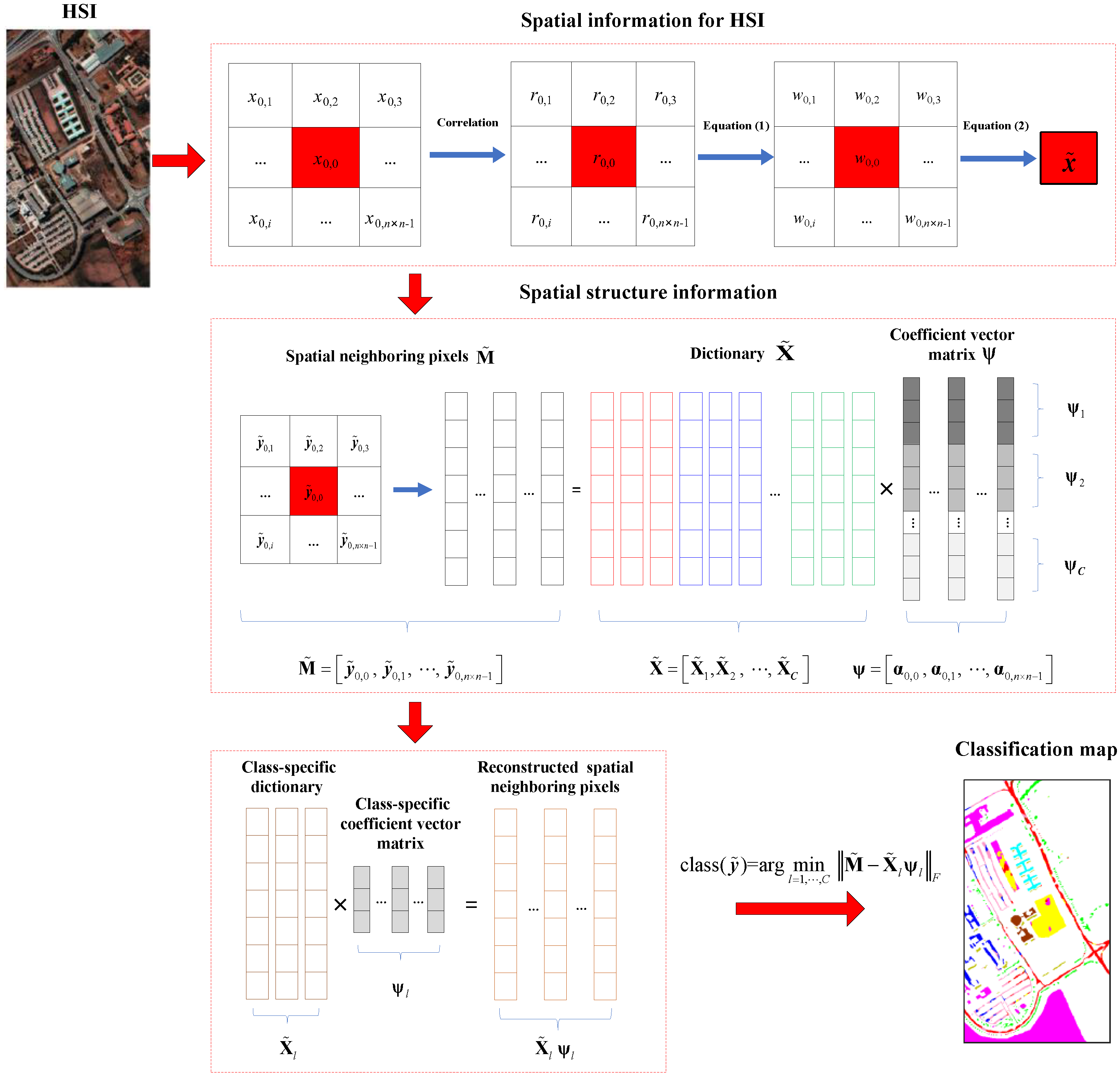
To fully mine the spatial–spectral features for HSI to assist with land cover classification, the proposed WSSJCRC method makes use of the superiorities of both WSSKCRT and JCRC methods. Firstly, as the same with WSSKCRT, the correlation coefficient-weighted spatial filtering operator constructed by Equation (1) and Equation (2) is utilized to perform spatial filtering on all pixels of HSI to alleviate the spectral shift caused by adjacency effect, so the training set X and the test sample y can be expressed as X ˜ = [ x ˜ 1 , x ˜ 2 , , x ˜ N ] R d × N and y ˜ R d × 1 , respectively.
Then, through the same method as JCRC, to take the spatial structure information for pixels into account the training set X ˜ is used to simultaneously represent the test sample y ˜ and its corresponding spatial neighboring pixels under the window of n × n, which can be written as
M ˜ = y ˜ 0 , 0   ,       y ˜ 0 ,   1 ,       y ˜ 0 , 2 ,           ,       y ˜ 0 , n × n 1       = X ˜ α 0 , 0   ,       α 0 , 1 ,       α 0 , 2 ,         ,       α 0 , n × n 1 ψ = X ˜ ψ
where y ˜ 0 , 0 represents the test sample y ˜ itself. Moreover, the coefficient vector matrix ψ is solved by the Frobenius norm, i.e.,
ψ = arg     min ψ M ˜ X ˜ ψ * F 2 + λ ψ F 2
The solution for ψ can be calculated with a closed-form solution as follows:
ψ = ( X ˜ T X ˜ + λ I ) 1 X ˜ T M ˜
Finally, the test sample y ˜ is assigned to the class with the minimum reconstruction error, i.e.,
class ( y ˜ ) = arg     min l = 1 , , C         M ˜ X ˜ l ψ l F
where X ˜ l = [ x ˜ l , 1 , x ˜ l , 2 , , x ˜ l , N l ] R d × N l represents the training set for the lth class after spatial filtering, and ψ l denotes the corresponding coefficient vector matrix for the lth class.
The flowchart for the proposed WSSJCRC method is shown in Figure 3.

2.4. Proposed WSSJKCRC

As mentioned in the Introduction, the hyperspectral data usually present in a nonlinear structure due to different topographic structures and surface roughness [35]. To enhance the separability of nonlinear hyperspectral data, the kernel version of WSSJCRC (i.e., WSSJKCRC) is proposed in this paper to project the hyperspectral data into the kernel-induced high-dimensional feature space, in which the coefficient vector matrix ψ can be solved by the optimization problem as follows:
ψ = arg     min ψ Φ ( M ˜ ) Φ ( X ˜ ) ψ * F 2 + λ ψ F 2
And the closed-form solution for ψ can be denoted as
ψ = ( K ( X ˜ ) + λ I ) 1 K ( X ˜ , M ˜ )
where K ( X ˜ ) = Φ ( X ˜ ) T Φ ( X ˜ ) R N × N is the Gram matrix formed from K ( X ˜ ) i , j = k ( x ˜ i , x ˜ j ) (i, j = 1, 2, …, N), and K ( X ˜ , M ˜ ) = Φ ( X ˜ ) T Φ ( M ˜ ) R N × N represents the matrix composed of K ( X ˜ , M ˜ ) i , j = k ( x ˜ i , y ˜ 0 , j ) , in which i = 1, 2, …, N, j = 0, 1, 2, …, N 1 , and N represents the number of spatial neighboring pixels under the window of n × n, i.e., N = n × n. Finally, the mapped spatial neighboring pixels Φ ( M ˜ ) for the test sample y ˜ are reconstructed by the mapped class-specific training samples Φ ( X ˜ l ) and the corresponding class-specific coefficient vector matrix ψ l , and then the test sample y ˜ is assigned to the class with the minimum reconstruction error, i.e.,
class (   y ˜ )   = arg     min l = 1 , , C         Φ ( X ˜ l ) ψ l Φ ( M ˜ ) F = arg     min l = 1 , , C         t r   ( ( Φ ( M ˜ ) Φ ( X ˜ l ) ψ l ) T ( Φ ( M ˜ ) Φ ( X ˜ l ) ψ l ) ) = arg     min l = 1 , , C         t r   ( K ( M ˜ ) + ψ l T K ( X ˜ l ) ψ l 2 ψ l T K ( X ˜ l , M ˜ ) )
where the symbol tr means to find the trace of square matrix, i.e., the sum of all the main diagonal elements for a square matrix, and K ( X ˜ l ) = Φ ( X ˜ l ) T Φ ( X ˜ l ) R N l × N l denotes the Gram matrix for the lth class, K ( M ˜ ) = Φ ( M ˜ ) T Φ ( M ˜ ) R N × N and K ( X ˜ l , M ˜ ) = Φ ( X ˜ l ) T Φ ( M ˜ ) R N l × N .
The flowchart for the proposed WSSJKCRC method is shown in Figure 4.

3. Experimental Results and Analysis

3.1. Experimental Data

In this paper, three real hyperspectral scenes are employed to evaluate the performance of the proposed methods.
The first land cover hyperspectral scene is Indian Pines. This hyperspectral scene was gathered by the Airborne Visible Infrared Imaging Spectrometer (AVIRIS) sensor over the Indian Pines test site in north-western Indiana. The scene image contains 145 × 145 pixels under a spatial resolution of 20 m, and provides 220 spectral bands in the range of 0.4–2.5 μm. After removing the bands covering the region of water absorption, 200 spectral bands are used for classification. The original ground truth map consists of 16 land cover classes. After eliminating some classes with very few samples, nine land cover classes are selected for the experiment in this paper. The false-color image and the ground truth map are shown in Figure 5a,b, respectively.
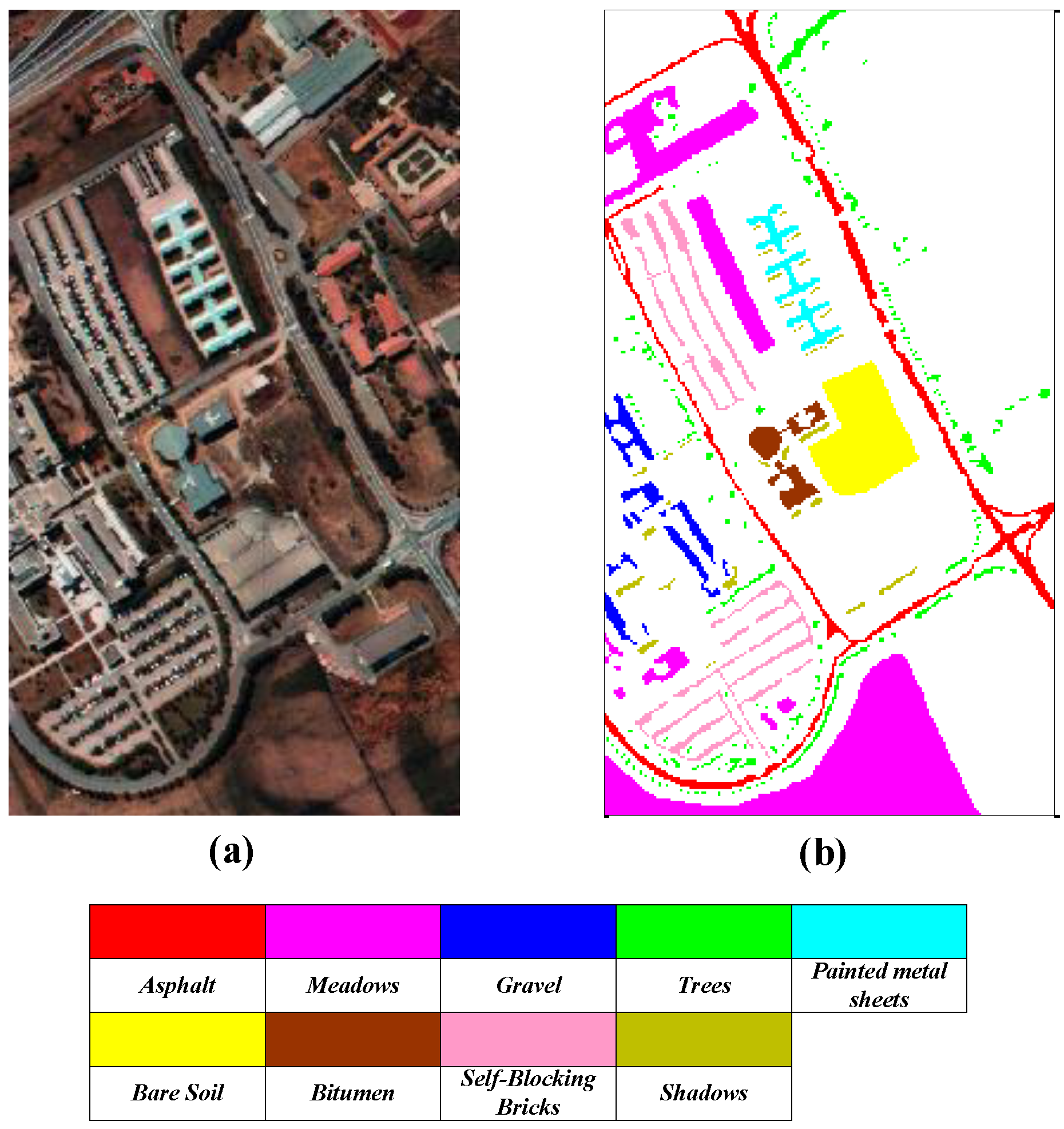
The second land cover hyperspectral scene is Pavia University. This scene was collected by Reflective Optics Spectrographic Imaging System (ROSIS) sensor in the University of Pavia, Pavia, Italy. Figure 6a shows the false-color image for the scene, which contains 610 × 340 pixels with a high spatial resolution of 1.3 m and consists of 103 spectral bands in the range of 0.43–0.86 μm. Moreover, there are nine land cover classes in the ground truth map shown in Figure 6b.
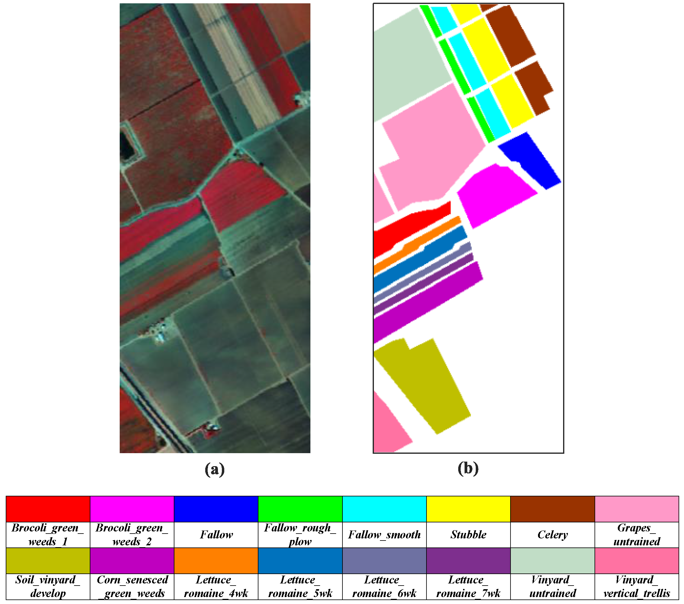
The last land cover hyperspectral scene is Salinas. This land cover scene was acquired by the AVIRIS sensor over Salinas Valley, California. The scene image contains 512 × 217 pixels with a spatial resolution of 3.7 m and provides 204 spectral bands after discarding the 20 water absorption bands. Its false-color image is shown in Figure 7a, and its ground truth map is shown in Figure 7b composed of 16 land cover classes.
In the ground truth maps as shown in Figure 5b, Figure 6b and Figure 7b, different colors represent different land cover types, in which the white areas represent unlabeled areas. It should be noted that it is time-consuming and expensive to label the pixels of HSI. Therefore, only major land cover types in the images are labeled, while non-major land types in the white areas are not labeled. The white areas are regarded as the background areas that are not considered as the classification targets. It should be emphasized that the white areas in Figure 5b contain not only unlabeled land types, but also some land types with very few samples. Moreover, each pixel in HSI is regarded as a sample.
Given the difficulty of labeling samples in HSI, this paper attempts to use small-scale labeled training samples to classify large-scale unlabeled test samples. For this reason, 5% of the labeled samples for each class are randomly selected as training samples in the Indian Pines scene, 60 labeled samples in each class are randomly picked as training samples in the Pavia University scene, and 20 labeled samples in each class are randomly chosen as training samples in the Salinas scene. The remaining samples are used as test samples in the corresponding hyperspectral scene. Table 1 shows the division of samples for three hyperspectral scenes.

3.2. Data Preprocessing

In practical hyperspectral scenes, different topographic structures and surface roughness lead to the amplitude shift, that is the shape and trend of spectral curves of the same ground object is nearly invariant but the reflectance level (i.e., spectral amplitude) varies considerably. The amplitude shift may produce an impact on the performance of classification models [35]. For simplicity, two kinds of ground objects are selected separately from the above-mentioned three hyperspectral scenes to illustrate the amplitude shift phenomenon, as shown in Figure 8a–f, i.e., (a) Hay-windrowed and (b) Woods for Indian Pines, (c) Painted metal sheets and (d) Self-Blocking Bricks for Pavia University, and (e) Fallow and (f) Stubble for Salinas. To alleviate such spectral shift, the above-mentioned three hyperspectral scenes are pretreated by the Amplitude Normalization (AN) method proposed in the reference [35]. After pretreatment with AN method, the amplitude difference is significantly reduced, that is the spectral curves for the same ground object become compact and concentrated, as shown in Figure 8g–l. Therefore, the pretreated data are used for subsequent modeling analysis to improve the performance of classification models.

3.3. Parameter Optimization

To fully verify the superiority of the proposed methods, the proposed WSSJCRC and WSSJKCRC methods are compared with the CRC, JCRC, CRC-M, JDKCRT, KCRT-CK, WSSDKCRT, and WSSKCRT methods on three real hyperspectral scenes for land cover classification performance. It should be noted that the essence of CRC-M is to introduce the directly averaging spatial filter operator into the CRC method, and other methods are all mentioned in the Introduction. To ensure the fairness of the experiment, the parameters of all methods are optimized, so that the classification performance of all methods can be compared under their respective optimal parameters.

3.3.1. Parameter Optimization of the Compared Methods

For the above-mentioned seven compared methods, namely CRC, JCRC, CRC-M, JDKCRT, KCRT-CK, WSSDKCRT, and WSSKCRT, there are four main parameters that affect the classification performance, i.e., global regularization parameter λ, positive regularization parameter β, spatial filtering window size Wf, and spatial structure window size Ws. According to the experience of relevant references in the Introduction, the optimization intervals of λ and β are set as {10−9, 10−8, 10−7, 10−6, 10−5, 10−4, 10−3, 10−2, 10−1, 1}, and the optimization intervals of Wf and Ws are set as {3 × 3, 5 × 5, 7 × 7, 9 × 9, 11 × 11, 13 × 13, 15 × 15, 17 × 17, 19 × 19, 21 × 21}. It should be noted that only the optimization interval of λ for CRC-M on the Salinas scene is set as {10−15, 10−14, 10−13, 10−12, 10−11, 10−10, 10−9, 10−8, 10−7, 10−6}. The corresponding parameters of each method are optimized by using training samples and five-fold cross-validation strategy, and the Overall Accuracy (OA) is used to evaluate the classification performance of each method under each parameter. The optimal parameter settings for the compared methods on the three hyperspectral scenes are shown in Table 2, where NA means that the corresponding parameter is not applied.

3.3.2. Parameter Optimization of the Proposed Methods

The proposed WSSJCRC and WSSJKCRC methods simultaneously include three main parameters that affect the classification performance, i.e., global regularization parameter λ, spatial filtering window size Wf, and spatial structure window size Ws. The optimization strategy and the optimization intervals of parameters are the same as those of the above-mentioned seven methods. Figure 9 shows the optimization process of the proposed WSSJCRC and WSSJKCRC methods on the Indian Pines, Pavia University, and Salinas scenes. In the three-dimensional graph as shown in Figure 9, the surface of different colors is used to represent the corresponding global regularization parameter λ, and the asterisk (*) is utilized to represent the position of the optimal parameters. The optimal parameter settings for the proposed methods on the three hyperspectral scenes are shown in Table 3.

3.4. Classification Results and Discussion

3.4.1. Analysis of Classification Performance

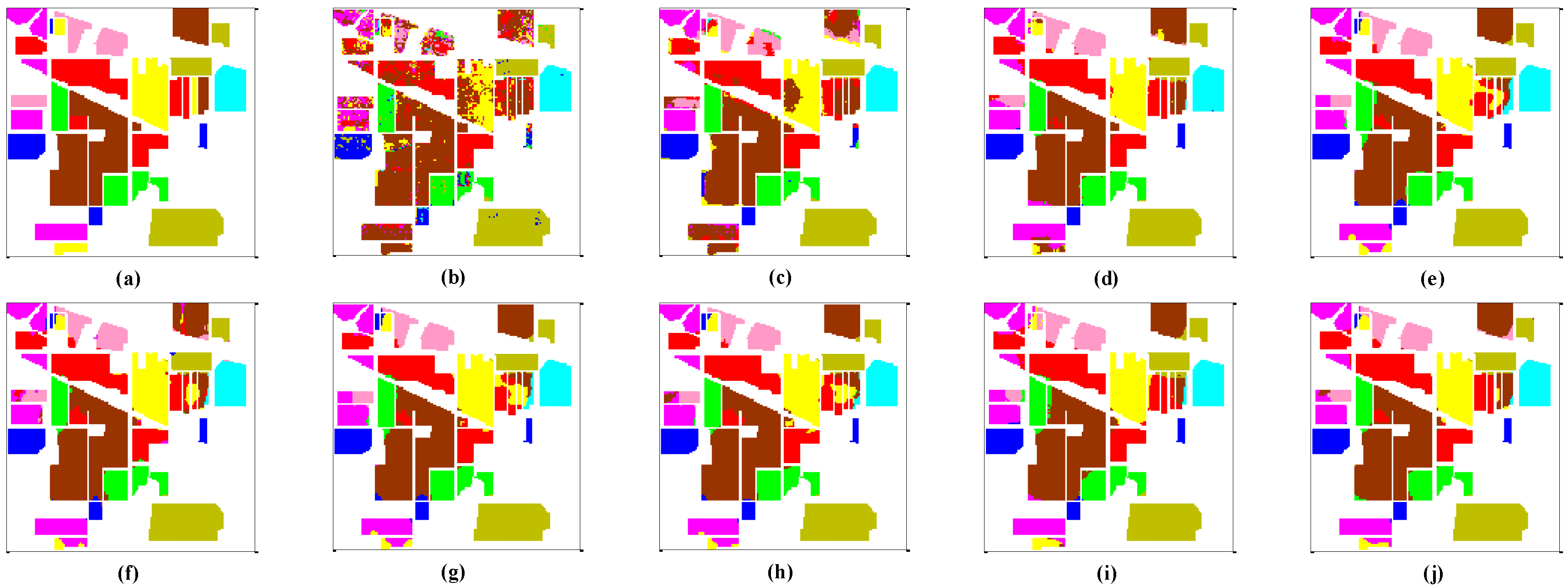
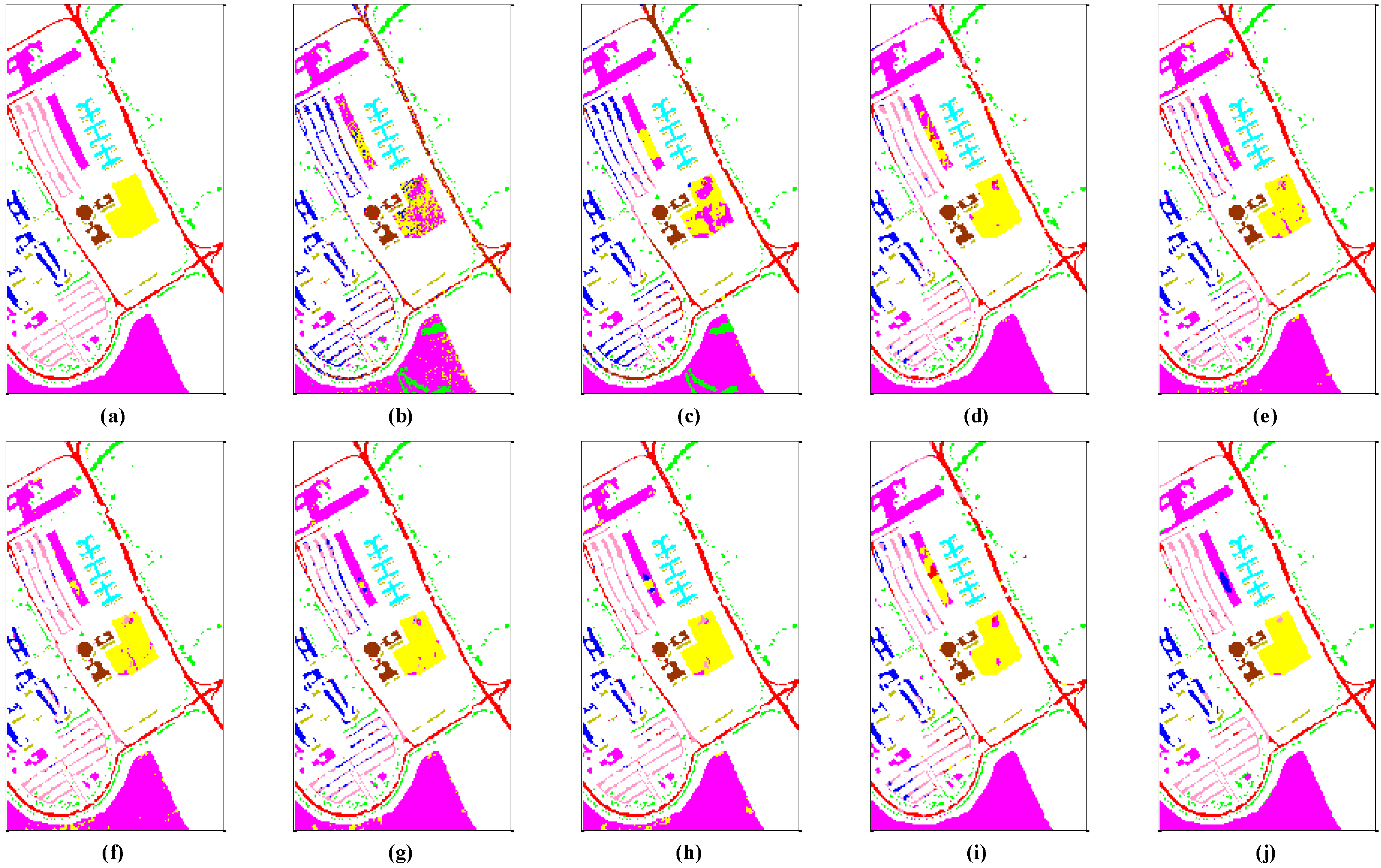
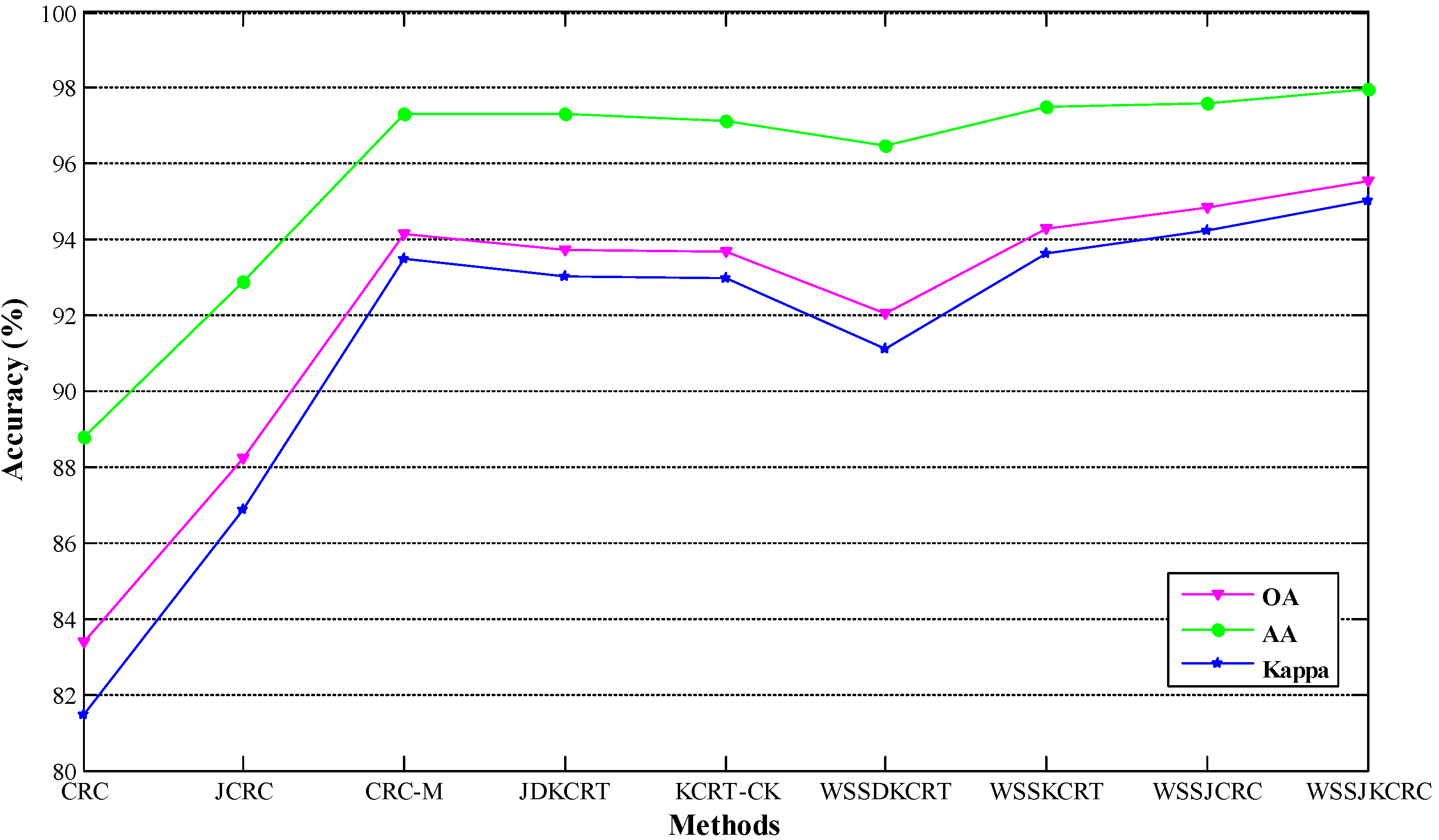
After parameter optimization, the above nine CR methods perform land cover classification with their respective optimal parameters on the Indian Pines, Pavia University, and Salinas scenes. Moreover, four evaluation indicators are utilized to evaluate the performance of each method for land cover classification, i.e., individual class accuracy, Overall Accuracy (OA), Average Accuracy (AA), and Kappa statistic (Kappa). Moreover, each method is performed repeatedly ten times and takes the average value as the final result to avoid random error and any bias. During each running process, training samples and test samples are randomly selected according to the proportion and number of samples set in Table 1. The land cover classification results of different methods are shown in Table 4, Figure 10 and Figure 11 for the Indian Pines scene, Table 5, Figure 12 and Figure 13 for the Pavia University scene, and Table 6, Figure 14 and Figure 15 for the Salinas scene, respectively. Among these figures, the curves of OA, AA, and Kappa values for each method on the three hyperspectral scenes are shown in Figure 10, Figure 12 and Figure 14. Moreover, the land cover classification maps generated by different methods on the three hyperspectral scenes are shown in Figure 11, Figure 13, and Figure 15, respectively.
It should be noted that in the process of HSI classification and mapping, the row number and column number of each pixel in HSI are used as the position index of the corresponding pixel. The spectral information of the training pixels and test pixels, as well as the labeling information of the training pixels, are extracted through the corresponding position index. The land cover classification model can be established according to the training pixels and their corresponding class labels. Moreover, the established model is employed to classify the test pixels, and the obtained class labels are placed on the corresponding positions in HSI according to the position index of the test pixels to complete the land cover classification mapping.
It can be seen from Table 4 and Figure 10, Table 5 and Figure 12, and Table 6 and Figure 14 that the proposed WSSJKCRC method achieves the best land cover classification performance on the three hyperspectral scenes, in which OA, AA, and Kappa reach 96.21%, 96.20%, and 0.9555 for the Indian Pines scene, 97.02%, 96.64%, and 0.9605 for the Pavia University scene, 95.55%, 97.97%, and 0.9504 for the Salinas scene, respectively. Moreover, the classification maps generated by WSSJKCRC contain the least noise and the most homogeneous areas, as shown in Figure 11j, Figure 13j and Figure 15j. Among all the methods, the CRC method produces the worst classification results on the three hyperspectral scenes, and there is a lot of noise in the classification maps produced by CRC shown in Figure 11b, Figure 13b and Figure 15b. The reason is that CRC only makes use of the spectral information of ground objects without considering any spatial information.
The CRC-M, JDKCRT, and KCRT-CK method perform spatial smoothing filtering on all pixels of HSI by directly averaging the spatial neighboring pixels, which reduces the noise in the original spectral curves of ground objects to a certain extent. Therefore, the classification performance of these three methods on the three hyperspectral scenes is significantly better than that of CRC, as shown in Table 4 and Figure 10, Table 5 and Figure 12, and Table 6 and Figure 14. However, these three methods do not consider the spectral shift caused by adjacency effect among the spatial neighboring pixels. As a result, the pixels in HSI contain a lot of noise. To alleviate such spectral shift, the WSSDKCRT and WSSKCRT methods utilize a weighted spatial filtering operator to perform spatial filtering on HSI. Moreover, the experimental results demonstrate that both WSSDKCRT and WSSKCRT achieve higher OA, AA, and Kappa than CRC-M, JDKCRT, and KCRT-CK on the Indian Pines and Pavia University scenes, as shown in Table 4 and Figure 10, and Table 5 and Figure 12. For the Salinas scene, WSSKCRT outperforms CRC-M, JDKCRT, and KCRT-CK, as shown in Table 6 and Figure 14. The CRC-M, JDKCRT, KCRT-CK, WSSDKCRT, and WSSKCRT methods consider the spatial information of HSI by taking the average or weighted average of spatial neighboring pixels of each pixel, but do not take the spatial structure information for pixels into account.
The JCRC method simultaneously represents each test pixel and its spatial neighborhood pixels through the labeled training pixels to consider the spatial structure information of each test pixel to assist the classification of the test pixel. Consequently, JCRC achieves much higher OA, AA, and Kappa than CRC on the three hyperspectral scenes. As with CRC, the JCRC method does not carry out spatial filtering operation on HSI, which leads to a large amount of noise in the spectral curves of ground objects. The proposed WSSJCRC method not only considers the spatial structure information, but also employes the weighted spatial filtering operator to filter the pixels in HSI. It can be seen from the experimental results that WSSJCRC significantly outperforms CRC and JCRC for land cover classification on the three hyperspectral scenes. Especially on the Salinas scene, the land cover classification performance of WSSJCRC is only inferior to that of WSSJKCRC.
On the basis of the proposed WSSJCRC method, the proposed WSSJKCRC method utilizes the kernel trick to project the sample data into a high-dimensional feature space, thereby enhancing the separability for nonlinear samples. This is the reason that WSSJKCRC achieves the best land cover classification performance on the three hyperspectral scenes among all the compared methods.
Moreover, all methods use small-scale labeled training samples to classify large-scale unlabeled test samples in the experiment. Moreover, the OA of WSSJKCRC reaches more than 95% on all the three hyperspectral scenes, which indicates that WSSJKCRC can achieve the promising performance for land cover classification with small-scale labeled samples.

3.4.2. Stability Analysis for Classification Performance

In this section, the standard deviation (STD) of the results for ten times is utilized to evaluate the stability of classification performance for each method. The lower the STD values of OA, AA, and Kappa for a certain method are, the more stable the classification performance of the method is.
On the Indian Pines scene, the STD values of OA and Kappa for the proposed WSSJKCRC method are lowest among all the methods as shown in Table 4. The STD value of AA for WSSJKCRC is lower than that of other methods except for the JDKCRT method. Although the STD value of AA for WSSJKCRC is slightly higher than that of JDKCRT, the STD values of OA and Kappa for WSSJKCRC is lower than those of JDKCRT. On the Pavia University scene, it can be seen from Table 5 that the STD values of OA, AA, and Kappa for WSSJKCRC are lower than those of JCRC and WSSJCRC. Moreover, the STD values of OA and Kappa for WSSJKCRC are lower than those of CRC, CRC-M, and KCRT-CK. On the Salinas scene, the STD values of OA, AA, and Kappa for the proposed WSSJKCRC method are basically similar to those of the CRC-M, KCRT-CK, and WSSJCRC methods, but much lower than those of other methods as shown in Table 6.
Therefore, it can be seen from the above analysis that the stability of classification performance for the proposed WSSJKCRC method is satisfactory.

3.4.3. Significance Analysis for Classification Performance

It can be seen from Table 4 and Figure 10, Table 5 and Figure 12, and Table 6 and Figure 14 that the proposed WSSJKCRC method obtains the highest OA, AA, and Kappa values among all the compared methods on the Indian Pines, Pavia University, and Salinas scenes, which indicates that the proposed WSSJKCRC method has better classification performance than other methods. To further illustrate the significant difference for the classification performance of the proposed WSSJKCRC method and other methods, the t-test is utilized for significance analysis between the OA, AA, and Kappa obtained by WSSJKCRC for ten times and the OA, AA, and Kappa obtained by other methods for ten times at the significance level of 0.05. The p-values for OA, AA, and Kappa for different methods on the three hyperspectral scenes are shown in Table 7, in which p-value that is less than 0.05 indicates that the classification performance for the proposed WSSJKCRC method is significantly different from that of the corresponding method.
As can be seen from Table 7, on the Indian Pines scene, the p-values for OA, AA, and Kappa between WSSJKCRC and WSSKCRT, and p-value for AA between WSSJKCRC and WSSDKCRT are higher than 0.05, but the p-values for OA, AA, and Kappa between WSSJKCRC and other methods are less than 0.05. On the Pavia University and Salinas scenes, the p-values for OA, AA, and Kappa between WSSJKCRC and other methods are all less than 0.05.
According to the classification results and the significance analysis of classification performance, the proposed WSSJKCRC method is not only better than other methods in classification performance, but also its classification performance is significantly different from other methods on the whole. Therefore, the proposed WSSJKCRC method is more advantageous than other comparison methods for HSI classification.

3.5. Comparison of Running Time

In this section, the running time for different methods is compared and analyzed on the Indian Pines, Pavia University, and Salinas scenes. All the methods are implemented using the MATLAB R2014a software on a computer with 2.90 GHz CPU and 32 GB RAM. To avoid random error and any bias, each method is performed repeatedly ten times and takes the average value of running time as the final result. The running time for these methods is shown in Table 8.
It can be seen from Table 8 that the proposed WSSJCRC and WSSJKCRC methods take more time than other methods on the three hyperspectral scenes. The main reason is that WSSJCRC and WSSJKCRC not only perform spatial filtering on HSI, but also consider the spatial structure information of each test pixel. Moreover, the larger the size of spatial filtering window Wf and spatial structure window Ws is, the more time WSSJCRC and WSSJKCRC take. However, the CRC-M, JDKCRT, KCRT-CK, WSSDKCRT, and WSSKCRT methods only perform spatial filtering on HSI, and JCRC only takes the spatial structure information of each test sample into account. Therefore, these methods take less time than the proposed WSSJCRC and WSSJKCRC methods. The CRC method only utilizes the spectral information of HSI for classification, but does not consider any spatial information, so its running time is the least.

4. Conclusions

To fully mine the spatial–spectral features for HSI, a novel WSSJCRC method is proposed for land cover classification in this paper, which not only utilizes a weighted spatial filtering operator to perform spatial filtering on HSI to alleviate the spectral shift caused by adjacency effect, but also considers the spatial structure information of each test pixel. On this basis, a WSSJKCRC method is also proposed, in which the kernel trick is introduced into the WSSJCRC method to enhance the separability of nonlinear samples. To verify the effectiveness of the proposed methods, the proposed WSSJCRC and WSSJKCRC methods are compared with seven traditional CR methods on three real hyperspectral scenes. According to the experimental results, it can be concluded as follows:
(1)
The proposed WSSJCRC method significantly outperforms the traditional CRC and JCRC methods for land cover classification on the three hyperspectral scenes;
(2)
The proposed WSSJKCRC method achieves the best land cover classification performance on the three hyperspectral scenes among all the compared methods. The OA, AA, and Kappa of WSSJKCRC reach 96.21%, 96.20%, and 0.9555 for the Indian Pines scene, 97.02%, 96.64%, and 0.9605 for the Pavia University scene, 95.55%, 97.97%, and 0.9504 for the Salinas scene, respectively;
(3)
WSSJKCRC can achieve the promising performance for land cover classification with OA over 95% on the three hyperspectral scenes under the situation of small-scale labeled samples, thus effectively reducing the labeling cost for HSI.
The experimental results on the three hyperspectral scenes demonstrate that the proposed WSSJCRC and WSSJKCRC methods can effectively improve the classification performance of CR model by considering both spatial filtering and spatial structure information for HSI. The proposed WSSJKCRC method achieves the best land cover classification performance among all the compared methods by introducing the kernel technique, and obtains the promising accuracy with small-scale labeled samples. However, this framework increases the complexity of CR model and makes the proposed WSSJCRC and WSSJKCRC methods take more time than other compared methods. In the subsequent studies, based on this framework and according to the references [18,23,34], we will develop effective nearest neighbor cooperative representation mechanisms to optimize the dictionary of CR model and exclude the classes and samples unrelated to test samples from the dictionary. This can not only further improve the classification performance of CR model, but also improve its operation efficiency.
In this paper, only three small airborne hyperspectral scenes are used to verify the land cover classification performance of the proposed methods. In future research, the wider-scale hyperspectral scenes will be utilized to verify the generalization performance of the proposed methods for land cover classification. Moreover, the application of CR models in land cover classification based on spaceborne HSI will be carried out, such as GF-5 and Hyperion. Furthermore, all bands in HSI are employed to establish the land cover classification models in this paper. However, hundreds of continuous bands in HSI are highly correlated, which may lead to the “Hughes phenomenon”, thus affecting the land cover classification performance of CR models. In the follow-up research, we will construct dimensionality reduction algorithms for hyperspectral data to select the important bands with low redundancy and a large amount of information. Moreover, land cover classification models will be established based on CR methods and these important bands to further improve the operation efficiency and classification performance of the models.

Author Contributions

Data curation, R.Y.; Methodology, R.Y.; Supervision, Q.Z. and Z.L.; Validation, B.F. and Y.W.; Writing—original draft, R.Y.; Writing—review and editing, R.Y. and B.F. All authors have read and agreed to the published version of the manuscript.

Funding

This work was supported by the Central Public-interest Scientific Institution Basal Research Fund (No. CAAS-ASTIP-2016-AII and No. JBYW-AII-2022-02) and the Project funded by China Postdoctoral Science Foundation (No. 2022M713415).

Institutional Review Board Statement

Not applicable.

Informed Consent Statement

Not applicable.

Data Availability Statement

The three real hyperspectral scenes used in this paper can be obtained from http://www.ehu.eus/ccwintco/index.php?title=Hyperspectral_Remote_Sensing_Scenes. And we obtained these datasets on 1 July 2021.

Acknowledgments

We acknowledge the Indian Pines, Pavia University, and Salinas hyperspectral scenes for the research of land cover classification.

Conflicts of Interest

The author declares no conflict of interest.

References

  1. Xie, S.; Liu, L.Y.; Zhang, X.; Yang, J.N. Mapping the annual dynamics of land cover in Beijing from 2001 to 2020 using Landsat dense time series stack. ISPRS J. Photogramm. Remote Sens. 2022, 185, 201–218. [Google Scholar] [CrossRef]
  2. Phan, T.N.; Kuch, V.; Lehnert, L.W. Land cover classification using google earth engine and random forest classifier-the role of image composition. Remote Sens. 2020, 12, 2411. [Google Scholar] [CrossRef]
  3. Agapiou, A. Land cover mapping from colorized CORONA archived greyscale satellite data and feature extraction classification. Land 2021, 10, 771. [Google Scholar] [CrossRef]
  4. Akar, O.; Gormus, E.T. Land use/land cover mapping from airborne hyperspectral images with machine learning algorithms and contextual information. Geocarto Int. 2022, 37, 3963–3990. [Google Scholar] [CrossRef]
  5. Wasniewski, A.; Hoscilo, A.; Chmielewska, M. Can a hierarchical classification of sentinel-2 data improve land cover mapping? Remote Sens. 2022, 14, 989. [Google Scholar] [CrossRef]
  6. Yu, Y.T.; Guan, H.Y.; Li, D.L.; Gu, T.N.; Wang, L.F.; Ma, L.F.; Li, J. A hybrid capsule network for land cover classification using multispectral LiDAR data. IEEE Geosci. Remote Sens. Lett. 2020, 17, 1263–1267. [Google Scholar] [CrossRef]
  7. Hong, D.F.; Hu, J.L.; Yao, J.; Chanussot, J.; Zhu, X.X. Multimodal remote sensing benchmark datasets for land cover classification with a shared and specific feature learning model. ISPRS J. Photogramm. Remote Sens. 2021, 178, 68–80. [Google Scholar] [CrossRef]
  8. Zafari, A.; Zurita-Milla, R.; Izquierdo-Verdiguier, E. Evaluating the performance of a random forest kernel for land cover classification. Remote Sens. 2019, 11, 575. [Google Scholar] [CrossRef] [Green Version]
  9. Li, X.Y.; Sun, C.; Meng, H.M.; Ma, X.; Huang, G.H.; Xu, X. A novel efficient method for land cover classification in fragmented agricultural landscapes using sentinel satellite imagery. Remote Sens. 2022, 14, 2045. [Google Scholar] [CrossRef]
  10. Lu, T.; Li, S.T.; Fang, L.Y.; Jia, X.P.; Benediktsson, J.A. From subpixel to superpixel: A novel fusion framework for hyperspectral image classification. IEEE Trans. Geosci. Remote Sens. 2017, 55, 4398–4411. [Google Scholar] [CrossRef]
  11. Gao, Q.S.; Lim, S.; Jia, X.P. Improved joint sparse models for hyperspectral image classification based on a novel neighbour selection strategy. Remote Sens. 2018, 10, 905. [Google Scholar] [CrossRef] [Green Version]
  12. Yu, H.Y.; Shang, X.D.; Song, M.P.; Hu, J.C.; Jiao, T.; Guo, Q.D.; Zhang, B. Union of class-dependent collaborative representation based on maximum margin projection for hyperspectral imagery classification. IEEE J. Sel. Top. Appl. Earth Observ. Remote Sens. 2021, 14, 553–566. [Google Scholar] [CrossRef]
  13. Bigdeli, B.; Samadzadegan, F.; Reinartz, P. A multiple SVM system for classification of hyperspectral remote sensing data. J. Indian Soc. Remote Sens. 2013, 41, 763–776. [Google Scholar] [CrossRef] [Green Version]
  14. Waske, B.; van der Linden, S.; Benediktsson, J.A.; Rabe, A.; Hostert, P. Sensitivity of support vector machines to random feature selection in classification of hyperspectral data. IEEE Trans. Geosci. Remote Sens. 2010, 48, 2880–2889. [Google Scholar] [CrossRef] [Green Version]
  15. Lopez-Fandino, J.; Quesada-Barriuso, P.; Heras, D.B.; Arguello, F. Efficient ELM-based techniques for the classification of hyperspectral remote sensing images on commodity GPUs. IEEE J. Sel. Top. Appl. Earth Observ. Remote Sens. 2015, 8, 2884–2893. [Google Scholar] [CrossRef]
  16. Huang, F.; Lu, J.; Tao, J.; Li, L.; Tan, X.C.; Liu, P. Research on optimization methods of ELM classification algorithm for hyperspectral remote sensing images. IEEE Access 2019, 7, 108070–108089. [Google Scholar] [CrossRef]
  17. Zhang, Y.Q.; Cao, G.; Li, X.S.; Wang, B.S. Cascaded random forest for hyperspectral image classification. IEEE J. Sel. Top. Appl. Earth Observ. Remote Sens. 2018, 11, 1082–1094. [Google Scholar] [CrossRef]
  18. Li, W.; Du, Q.; Zhang, F.; Hu, W. Collaborative-representation-based nearest neighbor classifier for hyperspectral imagery. IEEE Geosci. Remote Sens. Lett. 2015, 12, 389–393. [Google Scholar] [CrossRef]
  19. Su, H.J.; Zhao, B.; Du, Q.; Du, P.J. Kernel collaborative representation with local correlation features for hyperspectral image classification. IEEE Trans. Geosci. Remote Sens. 2019, 57, 1230–1241. [Google Scholar] [CrossRef]
  20. Ye, M.C.; Qian, Y.T.; Zhou, J.; Tang, Y.Y. Dictionary learning-based feature-level domain adaptation for cross-scene hyperspectral image classification. IEEE Trans. Geosci. Remote Sens. 2017, 55, 1544–1562. [Google Scholar] [CrossRef] [Green Version]
  21. Chen, H.; Ye, M.C.; Lei, L.; Lu, H.J.; Qian, Y.T. Semisupervised dual-dictionary learning for heterogeneous transfer learning on cross-scene hyperspectral images. IEEE J. Sel. Top. Appl. Earth Observ. Remote Sens. 2020, 13, 3164–3178. [Google Scholar] [CrossRef]
  22. Shen, J.Y.; Cao, X.B.; Li, Y.; Xu, D. Feature adaptation and augmentation for cross-scene hyperspectral image classification. IEEE Geosci. Remote Sens. Lett. 2018, 15, 622–626. [Google Scholar] [CrossRef]
  23. Yang, R.C.; Zhou, Q.B.; Fan, B.L.; Wang, Y.T. Land cover classification from hyperspectral images via local nearest neighbor collaborative representation with Tikhonov regularization. Land 2022, 11, 702. [Google Scholar] [CrossRef]
  24. He, X.; Chen, Y.S. Transferring CNN ensemble for hyperspectral image classification. IEEE Geosci. Remote Sens. Lett. 2021, 18, 876–880. [Google Scholar] [CrossRef]
  25. Sun, H.; Zheng, X.T.; Lu, X.Q. A supervised segmentation network for hyperspectral image classification. IEEE Trans. Image Process. 2021, 30, 2810–2825. [Google Scholar] [CrossRef] [PubMed]
  26. Du, P.J.; Gan, L.; Xia, J.S.; Wang, D.M. Multikernel adaptive collaborative representation for hyperspectral image classification. IEEE Trans. Geosci. Remote Sens. 2018, 56, 4664–4677. [Google Scholar] [CrossRef]
  27. Li, W.; Du, Q.; Zhang, F.; Hu, W. Hyperspectral image classification by fusing collaborative and sparse representations. IEEE J. Sel. Top. Appl. Earth Observ. Remote Sens. 2016, 9, 4178–4187. [Google Scholar] [CrossRef]
  28. Chen, X.; Li, S.Y.; Peng, J.T. Hyperspectral imagery classification with multiple regularized collaborative representations. IEEE Geosci. Remote Sens. Lett. 2017, 14, 1121–1125. [Google Scholar] [CrossRef]
  29. Li, W.; Du, Q.; Xiong, M.M. Kernel collaborative representation with Tikhonov regularization for hyperspectral image classification. IEEE Geosci. Remote Sens. Lett. 2015, 12, 48–52. [Google Scholar]
  30. Wright, J.; Yang, A.Y.; Ganesh, A.; Sastry, S.S.; Ma, Y. Robust face recognition via sparse representation. IEEE Trans. Pattern Anal. Mach. Intell. 2009, 31, 210–227. [Google Scholar] [CrossRef] [PubMed] [Green Version]
  31. Zhang, L.; Yang, M.; Feng, X.C. Sparse representation or collaborative representation: Which helps face recognition? In Proceedings of the IEEE International Conference on Computer Vision, Barcelona, Spain, 6–13 November 2011; pp. 471–478. [Google Scholar]
  32. Li, W.; Tramel, E.W.; Prasad, S.; Fowler, J.E. Nearest regularized subspace for hyperspectral classification. IEEE Trans. Geosci. Remote Sens. 2014, 52, 477–489. [Google Scholar] [CrossRef] [Green Version]
  33. Li, W.; Zhang, Y.X.; Liu, N.; Du, Q.; Tao, R. Structure-aware collaborative representation for hyperspectral image classification. IEEE Trans. Geosci. Remote Sens. 2019, 57, 7246–7261. [Google Scholar] [CrossRef]
  34. Yang, R.C.; Kan, J.M. Euclidean distance-based adaptive collaborative representation with Tikhonov regularization for hyperspectral image classification. Multimed. Tools Appl. 2022. [Google Scholar] [CrossRef]
  35. Liu, H.; Li, W.; Xia, X.G.; Zhang, M.M.; Gao, C.Z.; Tao, R. Spectral shift mitigation for cross-scene hyperspectral imagery classification. IEEE J. Sel. Top. Appl. Earth Observ. Remote Sens. 2021, 14, 6624–6638. [Google Scholar] [CrossRef]
  36. Ma, Y.; Li, C.; Li, H.; Mei, X.G.; Ma, J.Y. Hyperspectral image classification with discriminative kernel collaborative representation and Tikhonov regularization. IEEE Geosci. Remote Sens. Lett. 2018, 15, 587–591. [Google Scholar] [CrossRef]
  37. Su, H.J.; Hu, Y.Z.; Lu, H.L.; Sun, W.W.; Du, Q. Diversity-driven multikernel collaborative representation ensemble for hyperspectral image classification. IEEE J. Sel. Top. Appl. Earth Observ. Remote Sens. 2022, 15, 2861–2876. [Google Scholar] [CrossRef]
  38. Li, W.; Du, Q. Joint within-class collaborative representation for hyperspectral image classification. IEEE J. Sel. Top. Appl. Earth Observ. Remote Sens. 2014, 7, 2200–2208. [Google Scholar] [CrossRef]
  39. Shaw, G.A.; Burke, H.K. Spectral imaging for remote sensing. Lincoln Lab. J. 2003, 14, 3–28. [Google Scholar]
  40. Yang, R.C.; Fan, B.L.; Wei, R.; Wang, Y.T.; Zhou, Q.B. Land cover classification from hyperspectral images via weighted spatial-spectral kernel collaborative representation with Tikhonov regularization. Land 2022, 11, 263. [Google Scholar] [CrossRef]
  41. Yang, J.H.; Qian, J.X. Hyperspectral image classification via multiscale joint collaborative representation with locally adaptive dictionary. IEEE Geosci. Remote Sens. Lett. 2018, 15, 112–116. [Google Scholar] [CrossRef]
Figure 1. The flowchart for the WSSKCRT method.
Agriculture 13 00304 g001
Figure 2. The flowchart for the JCRC method.
Agriculture 13 00304 g002
Figure 3. The flowchart for the proposed WSSJCRC method.
Agriculture 13 00304 g003
Figure 4. The flowchart for the proposed WSSJKCRC method.
Agriculture 13 00304 g004
Figure 5. The Indian Pines scene: (a) false-color image and (b) ground truth map.
Agriculture 13 00304 g005
Figure 6. The Pavia University scene: (a) false-color image and (b) ground truth map.
Agriculture 13 00304 g006
Figure 7. The Salinas scene: (a) false-color image and (b) ground truth map.
Agriculture 13 00304 g007
Figure 8. Original spectral curves: (a) Hay-windrowed and (b) Woods for Indian Pines, (c) Painted metal sheets and (d) Self-Blocking Bricks for Pavia University, and (e) Fallow and (f) Stubble for Salinas; and pretreated spectral curves with AN: (g) Hay-windrowed and (h) Woods for Indian Pines, (i) Painted metal sheets and (j) Self-Blocking Bricks for Pavia University, and (k) Fallow and (l) Stubble for Salinas.
Agriculture 13 00304 g008
Figure 9. Classification performance under different parameters: (a) WSSJCRC and (d) WSSJKCRC on the Indian Pines scene, (b) WSSJCRC and (e) WSSJKCRC on the Pavia University scene, and (c) WSSJCRC and (f) WSSJKCRC on the Salinas scene.
Agriculture 13 00304 g009
Figure 10. The OA, AA, and Kappa values for different methods on the Indian Pines scene.
Agriculture 13 00304 g010
Figure 11. Land cover classification maps generated by different methods on the Indian Pines scene: (a) ground truth, (b) CRC, (c) JCRC, (d) CRC-M, (e) JDKCRT, (f) KCRT-CK, (g) WSSDKCRT, (h) WSSKCRT, (i) WSSJCRC, and (j) WSSJKCRC.
Agriculture 13 00304 g011
Figure 12. The OA, AA, and Kappa values for different methods on the Pavia University scene.
Agriculture 13 00304 g012
Figure 13. Land cover classification maps generated by different methods on the Pavia University scene: (a) ground truth, (b) CRC, (c) JCRC, (d) CRC-M, (e) JDKCRT, (f) KCRT-CK, (g) WSSDKCRT, (h) WSSKCRT, (i) WSSJCRC, and (j) WSSJKCRC.
Agriculture 13 00304 g013
Figure 14. The OA, AA, and Kappa values for different methods on the Salinas scene.
Agriculture 13 00304 g014
Figure 15. Land cover classification maps generated by different methods on the Salinas scene: (a) ground truth, (b) CRC, (c) JCRC, (d) CRC-M, (e) JDKCRT, (f) KCRT-CK, (g) WSSDKCRT, (h) WSSKCRT, (i) WSSJCRC, and (j) WSSJKCRC.
Agriculture 13 00304 g015
Table 1. The division of samples for the Indian Pines, Pavia University, and Salinas scenes.
Indian PinesPavia UniversitySalinas
No.ClassTraining SamplesTest SamplesNo.ClassTraining SamplesTest SamplesNo.ClassTraining SamplesTest Samples
1Corn-notill7213561Asphalt6065711Brocoli_green_weeds_1201949
2Corn-mintill427882Meadows6018,5892Brocoli_green_weeds_2203666
3Grass-pasture254583Gravel6020393Fallow201916
4Grass-trees376934Trees6030044Fallow_rough_plow201334
5Hay-windrowed244545Painted metal sheets6012855Fallow_smooth202618
6Soybean-notill499236Bare Soil6049696Stubble203899
7Soybean-mintill12323327Bitumen6012707Celery203519
8Soybean-clean305638Self-Blocking Bricks6036228Grapes_untrained2011,211
9Woods6412019Shadows608879Soil_vinyard_develop206143
10Corn_senesced_green_weeds203218
11Lettuce_romaine_4wk201008
12Lettuce_romaine_5wk201867
13Lettuce_romaine_6wk20856
14Lettuce_romaine_7wk201010
15Vinyard_untrained207208
16Vinyard_vertical_trellis201747
All class4668768 All class54042,236 All class32053,169
Table 2. Optimal parameter settings for the compared methods on the Indian Pines, Pavia University, and Salinas scenes.
MethodIndian PinesPavia UniversitySalinas
λβWfWsλβWfWsλβWfWs
CRC10−6NANANA10−5NANANA10−7NANANA
JCRC10−7NANA7 × 710−7NANA5 × 510−8NANA3 × 3
CRC-M10−8NA13 × 13NA10−8NA13 × 13NA10−11NA11 × 11NA
JDKCRT10−310−219 × 19NA10−310−45 × 5NA10−410−49 × 9NA
KCRT-CK10−5NA15 × 15NA10−2NA5 × 5NA10−3NA9 × 9NA
WSSDKCRT10−410−319 × 19NA10−310−47 × 7NA10−310−45 × 5NA
WSSKCRT10−4NA19 × 19NA10−2NA9 × 9NA10−8NA9 × 9NA
Table 3. Optimal parameter settings for the proposed WSSJCRC and WSSJKCRC methods on the Indian Pines, Pavia University, and Salinas scenes.
MethodIndian PinesPavia UniversitySalinas
λWfWsλWfWsλWfWs
WSSJCRC10−821 × 2113 × 1310−713 × 133 × 310−911 × 117 × 7
WSSJKCRC10−315 × 157 × 710−413 × 137 × 710−411 × 117 × 7
Table 4. Land cover classification accuracy with STD for different methods on the Indian Pines scene.
ClassCRCJCRCCRC-MJDKCRTKCRT-CKWSSDKCRTWSSKCRTWSSJCRCWSSJKCRC
164.76
± 4.26
83.33
± 4.65
89.73
± 2.24
89.59
± 2.16
92.88
± 1.41
91.57
± 2.17
93.25
± 3.16
85.96
± 3.90
92.43
± 1.98
232.60
± 6.43
60.36
± 3.33
94.24
± 2.59
94.71
± 1.77
94.09
± 2.98
94.49
± 4.42
95.66
± 2.86
92.54
± 2.63
94.51
± 1.57
376.92
± 5.27
88.47
± 2.81
92.29
± 4.66
95.87
± 3.05
94.17
± 4.50
96.83
± 2.06
97.88
± 2.43
93.08
± 5.74
95.44
± 3.76
491.24
± 2.36
98.56
± 0.86
98.82
± 1.02
97.73
± 0.83
97.59
± 1.45
97.60
± 1.69
96.22
± 2.31
97.53
± 1.12
98.25
± 1.04
598.37
± 1.03
100.00
± 0.00
99.91
± 0.26
99.71
± 0.36
98.96
± 1.40
99.49
± 0.69
99.01
± 1.27
99.96
± 0.13
99.98
± 0.07
642.05
± 5.23
62.95
± 6.19
90.10
± 2.61
92.09
± 2.41
93.43
± 2.57
93.10
± 2.54
93.38
± 2.41
87.28
± 2.26
92.29
± 2.56
781.93
± 1.82
86.42
± 1.84
97.36
± 0.76
95.19
± 1.49
96.24
± 1.35
95.81
± 1.28
96.83
± 1.63
93.66
± 2.19
97.94
± 1.20
818.76
± 3.63
65.56
± 6.54
93.21
± 3.62
94.33
± 3.16
92.38
± 4.05
94.03
± 3.24
92.65
± 6.42
88.56
± 4.07
95.74
± 1.95
997.31
± 0.67
99.92
± 0.07
99.74
± 0.47
99.15
± 0.76
98.23
± 0.94
99.41
± 0.42
99.13
± 0.94
99.06
± 0.76
99.20
± 0.46
OA (%)70.02
± 0.66
83.41
± 0.77
95.18
± 0.58
94.91
± 0.56
95.40
± 0.52
95.51
± 0.64
95.98
± 0.92
92.71
± 0.90
96.21
± 0.44
AA (%)67.10
± 0.80
82.84
± 0.88
95.04
± 0.83
95.38
± 0.44
95.33
± 0.67
95.82
± 0.66
96.00
± 1.14
93.07
± 1.05
96.20
± 0.52
Kappa0.6395
± 0.0086
0.8031
± 0.0092
0.9433
± 0.0069
0.9404
± 0.0065
0.9459
± 0.0060
0.9474
± 0.0074
0.9527
± 0.0108
0.9145
± 0.0106
0.9555
± 0.0052
Note: the best results are presented in bold font.
Table 5. Land cover classification accuracy with STD for different methods on the Pavia University scene.
ClassCRCJCRCCRC-MJDKCRTKCRT-CKWSSDKCRTWSSKCRTWSSJCRCWSSJKCRC
126.08
± 6.00
41.70
± 8.62
72.75
± 4.04
92.15
± 1.57
91.62
± 2.39
93.68
± 1.81
91.41
± 2.63
72.42
± 2.80
94.03
± 2.23
278.54
± 3.75
82.10
± 3.43
93.85
± 3.21
95.76
± 1.29
93.77
± 2.84
97.34
± 1.48
96.57
± 1.44
91.42
± 2.93
98.20
± 1.15
391.44
± 1.39
95.52
± 2.18
93.29
± 2.94
95.27
± 1.35
87.68
± 1.55
96.58
± 1.29
90.30
± 2.41
96.38
± 1.22
95.23
± 3.00
495.27
± 1.74
96.69
± 1.06
91.23
± 1.58
96.77
± 1.44
96.32
± 1.23
96.82
± 0.87
97.15
± 0.88
92.71
± 1.27
95.32
± 1.24
599.89
± 0.07
100.00
± 0.00
99.84
± 0.06
100.00
± 0.00
99.98
± 0.03
99.77
± 0.13
99.67
± 0.07
100.00
± 0.00
99.98
± 0.04
652.76
± 6.60
69.48
± 3.53
98.25
± 1.52
94.90
± 1.90
93.25
± 1.34
96.88
± 0.94
95.95
± 1.38
98.73
± 0.87
99.29
± 0.96
788.38
± 3.22
98.17
± 0.47
99.75
± 0.26
98.77
± 0.49
96.83
± 1.22
99.15
± 0.53
97.70
± 0.77
99.96
± 0.12
99.98
± 0.05
818.39
± 3.95
22.73
± 5.69
77.63
± 3.06
67.10
± 5.28
88.80
± 2.21
71.48
± 4.94
91.22
± 1.56
73.96
± 3.77
94.50
± 3.74
990.20
± 2.07
98.56
± 0.77
90.86
± 1.66
99.59
± 0.22
99.59
± 0.16
98.55
± 0.66
97.77
± 0.67
93.45
± 1.92
93.25
± 1.57
OA (%)65.19
± 1.47
72.30
± 1.43
89.78
± 1.58
92.99
± 0.60
93.24
± 1.18
94.58
± 0.56
95.13
± 0.63
88.72
± 1.53
97.02
± 0.77
AA (%)71.22
± 0.57
78.33
± 0.94
90.83
± 0.67
93.37
± 0.52
94.20
± 0.37
94.47
± 0.37
95.30
± 0.20
91.00
± 0.78
96.64
± 0.70
Kappa0.5547
± 0.0148
0.6442
± 0.0172
0.8656
± 0.0199
0.9073
± 0.0077
0.9109
± 0.0150
0.9282
± 0.0073
0.9355
± 0.0082
0.8525
± 0.0194
0.9605
± 0.0102
Note: the best results are presented in bold font.
Table 6. Land cover classification accuracy with STD for different methods on the Salinas scene.
ClassCRCJCRCCRC-MJDKCRTKCRT-CKWSSDKCRTWSSKCRTWSSJCRCWSSJKCRC
198.65
± 0.43
99.17
± 0.26
100.00
± 0.00
99.16
± 0.96
98.79
± 1.01
99.68
± 0.39
98.76
± 1.51
100.00
± 0.00
99.73
± 0.44
299.20
± 0.63
99.99
± 0.01
99.99
± 0.02
99.45
± 0.61
99.25
± 1.02
99.80
± 0.19
99.88
± 0.11
100.00
± 0.00
99.93
± 0.07
392.62
± 2.57
98.48
± 1.59
99.87
± 0.23
99.54
± 0.36
99.92
± 0.10
99.88
± 0.11
99.78
± 0.27
100.00
± 0.00
99.78
± 0.16
496.26
± 1.24
98.45
± 0.91
99.03
± 0.75
99.11
± 0.67
99.03
± 0.54
99.60
± 0.32
99.00
± 0.63
99.74
± 0.22
97.93
± 0.39
596.53
± 1.32
98.14
± 0.79
95.91
± 1.54
96.21
± 2.18
96.48
± 4.62
97.23
± 1.88
97.46
± 1.09
96.98
± 1.55
98.42
± 1.00
699.91
± 0.06
99.99
± 0.02
99.95
± 0.09
99.69
± 0.69
99.35
± 1.40
99.26
± 1.02
98.94
± 1.60
99.86
± 0.27
98.76
± 2.80
799.82
± 0.06
99.92
± 0.04
99.99
± 0.03
98.68
± 0.91
98.10
± 0.98
99.15
± 0.45
99.24
± 0.45
100.00
± 0.00
99.35
± 0.44
865.41
± 7.32
79.27
± 6.64
82.62
± 3.61
77.77
± 8.09
80.38
± 2.88
77.79
± 4.44
81.82
± 3.91
87.24
± 3.18
86.78
± 3.51
999.71
± 0.24
99.97
± 0.10
99.98
± 0.03
99.62
± 0.38
99.45
± 0.57
99.53
± 0.51
99.81
± 0.10
99.99
± 0.02
99.90
± 0.19
1086.79
± 1.40
91.33
± 1.18
95.93
± 2.60
97.96
± 0.93
97.44
± 1.47
95.99
± 1.40
97.51
± 1.67
96.14
± 2.60
97.39
± 1.54
1195.46
± 1.15
97.65
± 1.24
99.76
± 0.27
99.54
± 0.94
100.00
± 0.00
99.20
± 0.73
99.75
± 0.30
99.66
± 0.49
100.00
± 0.00
1271.75
± 5.26
89.04
± 5.23
99.26
± 0.43
99.87
± 0.32
99.97
± 0.04
100.00
± 0.00
99.77
± 0.40
99.14
± 1.10
99.96
± 0.04
1374.99
± 4.38
83.45
± 4.75
98.47
± 1.02
100.00
± 0.00
99.72
± 0.35
99.43
± 0.83
99.92
± 0.12
99.33
± 0.57
99.82
± 0.24
1490.67
± 1.92
95.89
± 2.05
99.39
± 0.52
98.66
± 1.04
98.82
± 0.93
96.90
± 3.07
99.16
± 0.68
97.97
± 2.05
99.19
± 1.19
1554.81
± 5.17
57.01
± 12.57
88.17
± 5.19
93.00
± 3.22
89.84
± 4.82
80.95
± 5.27
90.36
± 4.90
85.48
± 3.35
91.44
± 3.57
1697.70
± 0.60
98.44
± 0.45
99.14
± 0.76
99.11
± 0.54
97.82
± 2.43
99.14
± 0.67
98.75
± 0.98
99.93
± 0.08
99.07
± 1.52
OA (%)83.36
± 1.24
88.23
± 1.06
94.15
± 0.71
93.72
± 1.42
93.70
± 0.65
92.04
± 0.97
94.28
± 0.89
94.85
± 0.65
95.55
± 0.70
AA (%)88.77
± 0.60
92.89
± 0.72
97.34
± 0.27
97.34
± 0.37
97.15
± 0.48
96.47
± 0.51
97.49
± 0.38
97.59
± 0.29
97.97
± 0.30
Kappa0.8147
± 0.0134
0.8686
± 0.0120
0.9349
± 0.0079
0.9303
± 0.0157
0.9299
± 0.0073
0.9114
± 0.0108
0.9363
± 0.0099
0.9426
± 0.0073
0.9504
± 0.0078
Note: the best results are presented in bold font.
Table 7. Significance analysis of classification performance for the proposed WSSJKCRC method and other methods.
IndicatorsDatasetsCRCJCRCCRC-MJDKCRTKCRT-CKWSSDKCRTWSSKCRTWSSJCRC
p-value for OAIndian Pines4.110 × 10−261.082 × 10−194.661 × 10−43.155 × 10−51.961 × 10−31.423 × 10−24.923 × 10−14.526 × 10−9
Pavia
University
7.786 × 10−224.743 × 10−203.202 × 10−103.189 × 10−102.293 × 10−74.501 × 10−72.141 × 10−52.235 × 10−11
Salinas1.214 × 10−151.183 × 10−125.536 × 10−42.899 × 10−31.747 × 10−56.662 × 10−83.532 × 10−34.346 × 10−2
p-value for AAIndian Pines1.860 × 10−256.762 × 10−192.346 × 10−31.928 × 10−36.447 × 10−31.911 × 10−16.467 × 10−12.305 × 10−7
Pavia
University
6.868 × 10−252.903 × 10−205.771 × 10−131.280 × 10−92.867 × 10−81.531 × 10−73.041 × 10−53.740 × 10⁻¹²
Salinas2.773 × 10−191.637 × 10−132.110 × 10−48.763 × 10−43.891 × 10−45.278 × 10−79.463 × 10−31.542 × 10−2
p-value for KappaIndian Pines9.274 × 10−261.168 × 10−194.704 × 10−43.291 × 10−51.987 × 10−31.534 × 10−24.970 × 10−14.409 × 10−9
Pavia
University
4.011 × 10−232.287 × 10−201.875 × 10−102.673 × 10−101.705 × 10−73.780 × 10−71.969 × 10−51.577 × 10−11
Salinas8.783 × 10−161.351 × 10−125.487 × 10−42.894 × 10−31.839 × 10−56.549 × 10−83.596 × 10−34.189 × 10−2
Table 8. Running time (seconds) of different methods for land cover classification.
DatasetsCRCJCRCCRC-MJDKCRTKCRT-CKWSSDKCRTWSSKCRTWSSJCRCWSSJKCRC
Indian Pines0.4710.7513.4924.3315.3627.3427.904669.58463.77
Pavia University1.1049.6066.4050.6548.4852.1952.74211.301094.92
Salinas1.3818.0137.6329.2529.2248.7430.731136.041267.20
Disclaimer/Publisher’s Note: The statements, opinions and data contained in all publications are solely those of the individual author(s) and contributor(s) and not of MDPI and/or the editor(s). MDPI and/or the editor(s) disclaim responsibility for any injury to people or property resulting from any ideas, methods, instructions or products referred to in the content.