Abstract
To solve the problem of the lack of an accurate model for mechanized transportation and grading of walnut kernels, this paper took the shelled walnut kernels as the research object and calibrated the parameters of the discrete element model of walnut cracking kernels with the discrete element simulation software EDEM. The physical parameters of cracking kernels were measured by experiments, and the Hertz–Mindlin model was used to simulate the repose angle of cracking kernels. The contact parameters, such as the particle collision recovery coefficient, the static friction coefficient, and the rolling friction coefficient, were determined by the two-level factor test, steepest ascent test, and response surface test, respectively. Subsequently, the Hertz–Mindlin model with bonding contact was exploited to conduct the simulation of cracking kernels bending test based on the calibrated contact parameters. Finally, the normal contact stiffness, tangential contact stiffness, critical tangential force, and normal force of cracking kernels were determined by response surface analysis. It was shown that the relative error between the simulated values and the experiment results was 3.00 ± 1.31%. These results indicated that the calibrated parameter values are reliable, and could be used for the mechanized transportation and grading of walnut kernels.
1. Introduction
As one of the “four famous nuts” [1], walnut has rich unsaturated fatty acids. Regular consumption of walnuts helps to reduce blood pressure and blood lipids, and they are therefore favored by people [2]. The process of walnut production is generally divided into harvest, insecticide, storage, shelling, and grading [3,4,5,6]. However, walnut kernels with different particle sizes have different market values [7]. The whole and half walnut kernels with a large particle size can be directly packaged and sold because of their complete and beautiful appearance. Meanwhile, small particles of cracking kernels can be used as food processing accessories, such as walnut puree. Grading technology provides a potential way for an agricultural product to greatly increase its market value and promote the development of agriculture [8].
Manual grading is a low-efficiency and high-cost method for walnut kernels grading [9]. Vibration screening and rolling screening are commonly used grading approaches for agricultural products. But it is not suitable for walnut kernels because the large range in motion results in fracture and breakage [10], and then reduces the size and price of walnut kernels [11]. Thus, it is important to develop new machines with a small range of motion for walnut kernels grading [6]. In recent years, the discrete element method and the software EDEM have been widely used in the designing of agricultural machinery [12]. The discrete element method can be employed to obtain the hierarchical motion mechanism and provide a theoretical basis for the optimization of design parameters. For example, Liu et al. calibrated the parameters of the discrete element model for adzuki bean seeds and to design the seed metering device [13]. However, it is necessary to calibrate and determine the parameters of walnut kernels which were used in the EDEM before designing the grading machine.
The walnut kernels model with a different kernel size and different surface can be bonded by the particles with the same attribute [14,15,16,17]. The Hertz–Mindlin model of EDEM was used to establish the shape of sample, and subsequently, the bonding parameters were added to the Hertz–Mindlin model with bonding contact so that it can simulate the process of material breakage [18]. The basic parameters include Poisson’s ratio, shear modulus, and density, etc. The contact parameters mainly include the collision recovery coefficient, static friction coefficient, and dynamic friction coefficient. Furthermore, the bonding parameters include the normal phase and the tangential contact stiffness of the model, the normal tangential stress, and other bonding parameters. The accuracy of these parameters directly affects the design parameters of new machines [19].
Currently, there are few studies on the physical properties of walnut kernels. In this paper, the Xinjiang paper-skinned walnut was purchased from a local supermarket and taken as the research object. Using the EDEM software, we employed the Hertz–Mindlin model and the experimental results of the repose angle to choose the most significant parameters, collision recovery coefficient, static, and dynamic friction coefficients in order to conduct the steepest ascent test [20]. The Hertz–Mindlin model with bonding contact was then used to determine the normal phase, tangential stress, and other bonding parameters and to verify them with the bending tests [21].
2. Materials and Methods
2.1. Parametric Measurement
2.1.1. Sample of Walnut Kernels
The Xinjiang paper-skinned walnut, purchased from a local supermarket in Yangling, Xianyang City, Shaanxi Province, was used in this experiment. The walnut shell was shelled manually, and the density of walnut kernels was 0.972 ± 0.016 g/cm3 [7]. The long diameter, short diameter, and height of whole kernels were 33 ± 2.20, 27.33 ± 1.25, and 23.66 ± 1.71 mm, respectively [22]. A cutting knife was then taken to make cylindrical samples with a length of 10 mm and a radius of 7, 8, 9, and 10 mm for the compression test. The long diameter, short diameter, and height of the cracking kernels were 10.79 ± 2.37, 7.12 ± 2.33, and 5.56 ± 1.77 mm, respectively. The cracking kernels were collected for the repose angle measurement.
2.1.2. Compression Test
Using the cylindrical samples, we conducted a compression test with a texture meter (TA.XTC-16, Bosin Tech. Co., Ltd., Shanghai, China). The compression speed was 6 mm/min, and the loading displacement was set to 5 mm. Each test was repeated 10 times. According to the changes in height and diameter after uniaxial compression, the shear modulus of the walnut kernels was 1.87 ± 0.15 MPa, and the Poisson’s ratio was 0.40 ± 0.26.
2.1.3. Measurement of Repose Angle
The repose angle of the walnut kernels was obtained by the cylinder lifting method. During the measurement, the cylinder (d = 160 mm, H = 250 mm) was fixed on the universal material test bench, the bottom surface was contacted with the bottom of the test bench, and the cracking kernels were filled into it. The cylinder was lifted at a speed of 0.02 m/s so that the cracking kernels formed a repose angle, as shown in Figure 1. After five repetitions, the repose angle was θ = 37.58 ± 2.82°.
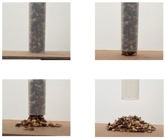
Figure 1.
Measurement of repose angle for walnut kernels.
2.1.4. Bending Test of Walnut Kernels
To obtain the parameter values of the bonding model, the texture meter was used to slowly apply loads to the cylindrical samples in supported cutting, and the maximum force was recorded as the destructive force. For the cylindrical samples, a customized cylindrical indenter was used for the bending test [21]. The distance between the fixed support points at both ends was 7 mm, and the load was applied at a speed of 0.001 m/s, as shown in Figure 2. Each test was repeated five times, and the average maximum destructive force was 34.4 ± 3.3 N.
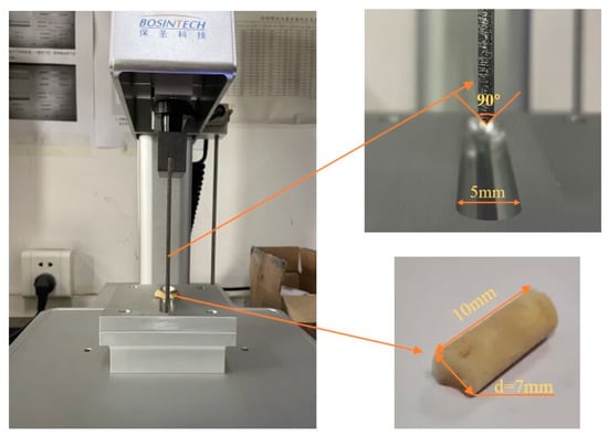
Figure 2.
The damage test of the walnut kernel.
2.2. Simulation Model
2.2.1. Simulation Model of the Repose Angle for Walnut Kernels
In the EDEM 2020 software, the Hertz–Mindlin model was applied to the repose angle simulation experiment. The Hertz–Mindlin model can calculate the motion and breaking of cracking kernels, as well as the bearing capacity between the sample particles. The main motions include the normal motion, tangential motion, and rolling motion between particles. To match the actual packing state, the cracking kernel model, shown in Figure 3, was established. Using a 3D scanner and its post-processing software, we obtained the point cloud data of the walnut kernel with a different integrity [23]. The point cloud data was then used to obtain the surface data of walnut kernels. The meshes for the broken walnut sample consisted of 10,245 domain elements, 1891 edge elements, and 325 end-point elements. Meanwhile, the automatic filling function of the EDEM software was used to obtain the collision model of the cracking kernels. The variation range of each simulation was determined by combining the physical property parameters of other agricultural products [24], as shown in Table 1. The model of the cracking kernel, shown in Figure 3, was established and the particle size distribution was specified as a normal distribution.
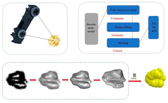
Figure 3.
The process of model building for cracking kernel.

Table 1.
The parameter range of the particle repose angle simulation model.
A virtual cylinder was established in the EDEM software as a particle factory (the inner diameter was 160 mm and the height was 250 mm), which dynamically generated cracking kernels at a speed of 0.3 kg/s and for a duration of 4 s. After the particle generation process was completed and had become stable, the cylinder was lifted at a speed of 0.02 m/s, and the particles were dropped to the bottom. The final stacking model is shown in Figure 4. The simulation was run on a workstation with two dual core Intel Xeon CPU 3.0 GHz processors, the 128 GB RAM with the Windows 10 64-bit operating system. It required approximately 25 min for each simulation.
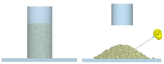
Figure 4.
The simulation process of the repose angle for cracking kernels.
2.2.2. Simulation of the Bending Test
The bending test of the cylindrical samples was conducted using the EDEM software. However, the rigid model established by the Hertz–Mindlin model cannot perform the bending test. Therefore, bonds were added to form a model with a mechanical strength based on the Hertz–Mindlin model. When the stress between the kernel particles reached the limit, the bond was broken.
The cylindrical sample model with bonds is shown in Figure 5. First, particles were bonded into the cylindrical sample model. The cylinder was drawn in the EDEM software and filled with adhesive particles with a radius of 1 mm. The cylinder was then compressed with a plate until it reached the required size. After the cylinder became stable, the bond was formed according to its adhesive radius. The model was then imported into a new file, and the indenter and the support plate, which have the same sizes during the bending test as above, were subsequently input. The spacing of the support plate was 7 mm, and the tool moved down at a speed of 0.002 m/s [25]. To establish the walnut kernel bending test, the Hertz–Mindlin with a bonding contact model was used; the parameter range is presented in Table 2.
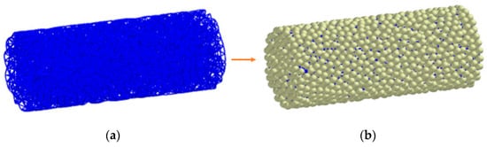
Figure 5.
The cylindrical sample model bonded by small particles: (a) bonds formed between particles, (b) cylindrical samples model with bonds.
Table 2.
The bond parameters of the walnut kernel bending failure simulation model.
2.3. Parameter Calibration Test Design
2.3.1. Calibration of the Basic Contact Parameters
A two-level test was used to combine all factors and all levels of each parameter to determine the main factor, which was defined as the change in output variables caused by the change of a factor at multiple levels. The software Design-Expert was used to conduct the two-level test in order to select the parameters which significantly affect the repose angle of cracking kernels. The repose angle simulation test was then established according to the parameters listed in Table 1, and the maximum and minimum values of the parameters were recorded. Here, 17 trials were designed.
Based on the above experimental results, the steepest ascent test was used to determine the main parameters, which were affected by the repose angle and identified the optimal area of cracking kernels [26]. For the non-significant parameters, the average value was substituted. The significant parameters were increased with the increasing step size. The repose angle test was then conducted, and the experimental repose angle was compared with the simulation repose angle and the relative error between simulated values and experimented results was determined. Finally, the optimal adjacent region was determined based on the less relative error.
A response surface test was conducted to determine the basic contact parameters [25]. According to the results of the above two experiments, the Box–Behnken Design (BBD) was used to implement the response surface test which was one of the second-level models of the response surface methodology. The maximum, minimum, and average optimal region was selected to carry out the repose angle experiment, and the average value of non-significant parameters was taken.
2.3.2. Response Surface Test for Bond Parameters
The Hertz–Mindlin model with a bonding contact is related to several parameters, including normal contact stiffness, tangential contact stiffness, critical normal force, and critical tangential force. Therefore, the Central Composite design (CCD) was designed to determine the parameter values, and the model was established based on the results of the contact parameters. Finally, the simulation and the crushing of walnut kernel were carried out. The codes of the bond parameters used in the simulation are listed in Table 3.
Table 3.
Coding of bond parameters.
3. Results and Discussion
3.1. Calibration of the Basic Contact Parameters
3.1.1. The Effects of Repose Angle on Parameter Screening
Here, nine parameters affecting the repose angle were used as test variables to conduct a two-level factor test design. The simulated results are presented in Table 4. The result indicated that the repose angle was 40.87 ± 5.75° and the error between the simulation results and the physical test values was less than 5%, which indicates that the test model is reliable.
Table 4.
The simulated results of the two-level test.
The effect of each parameter is presented in Table 5. According to the order of significance, three factors, namely, the rolling friction between cracking kernels, the static friction between the cracking kernels and the steel plate, and the shear modulus have significant effects on the repose angle in the test. Therefore, in the following experiment and the steepest ascent test, the above three factors were considered, and the other factors adopted as the average value. Specifically, the friction between walnut kernels was set to 0.8, the friction between the walnut kernel and the steel was set to 0.05, the coefficient of elasticity of walnut kernels was set to 0.3, the elastic recovery coefficient between the walnut kernel and the steel plate was set to 0.7, the Poisson’s ratio was set to 0.3, and the density was set to 950 kg/m3. Six values were determined by the two-level test, and in order to further calibrate the values with the significant influence of the repose angle, the steepest climbing experiment was needed.
Table 5.
The variance and effect of each parameter.
3.1.2. Steepest Ascent Test
The effect of the three factors on the repose angle was positive, i.e., the repose angle increased with the number of independent variables. The relative error of the repose angle in each experiment was observed and recorded. The results are presented in Table 6. As shown in Table 6, the relative error first decreased and then increased. Because the relative error of No. 4 was the lowest, the parameters values of No. 4 were taken as the centerpoint for the following tests. The results indicated that the correct parameter calibration value should be between tests 3 and 5. The BBD response surface test was carried out. The parameters values of No. 3 and No. 5 were regarded as the low and high levels, respectively.
Table 6.
The results of the steepest ascent test.
3.1.3. Results and Analysis of Response Surface Test
The software Design-Expert was employed to design the three-factor and three-level response of the surface test. The central value was set to five groups of repetitions, and a total of 17 groups of simulation tests were conducted. The experimental design and simulation results are shown in Table 7.
Table 7.
The results of steepest ascent test.
The response surface results were analyzed with the software Design-Expert, and the results of different mathematical models were compared. It was shown that the quadratic full model equation was the best-fitting equation. The results of ANOVA are listed in Table 8, and the equation was:
Table 8.
The analysis of variance for the regression equation.
It can be seen from Table 8 that the p-value of the quadratic full model was less than 0.01 and the p-value of the lack of fit term was more than 0.05, which indicates that the square terms of the three factors have a significant impact on the repose angle. Meanwhile, the p-value of the AB and AC term was less than 0.05. All of this indicates that the quadratic polynomial regression equation was established by accurately retaining all factors. This was consistent with the results of other agricultural products [24].
According to the repose angle test and the response surface analysis, the repose angle can be determined when the three parameters are known. However, these three parameters are contour surface curves. Furthermore, the analysis of the experimental and actual repose angle errors showed that the quadratic equation fits well; the coefficient of determination is R2 = 0.9469, and the equation was:
The results of ANOVA indicated that the p-value of the regression model was less than 0.05, and the p-value of the lack of fit was greater than 0.05, which proved that the model has a good fitness.
Through the mathematical solution function of Python software, the minimum point of the above equation can be calculated: the value of the repose angle was θ = 37.35 ± 2.32°. The relative error was 0.061%, which indicated that the difference between the simulation result and the actual one was less, and the contact parameter was feasible. The repose angle of the cracking kernel was slightly higher than that of wheat seeds [12] and sorghum seeds [22]. This may be caused by the irregular shape and surface of cracking kernels.
3.2. Calibration of Bond Parameters
According to the contact parameters, the CCD response surface test was designed to determine the phase contact stiffness, tangential contact stiffness, critical normal force, critical tangential force, as well as the other four bonding parameters. The bending simulation test was conducted, and three groups were set at the central level with a total of 30 groups of simulation tests. The design and simulation results of the bending test are presented in Table 9.
Table 9.
The design and results of a response surface for bond parameters.
The results of the fitting analysis indicated that the coefficient of determination was R2 = 0.9553. According to Table 10, the p-value of the full quadratic model was less than 0.01, and the lack of the fit term was more than 0.05. Therefore, the interaction terms of the four parameters and the square terms have significant effects on the results.
Table 10.
Quadratic full model analysis of variance on the response surface of bending test.
There were many factors which influenced the results of this equation. To ensure the significance of the model, the insignificant terms were eliminated. Subsequently, the regression equation can be described as:
Among the factors, the maximum shear stress, the interaction terms between the maximum shear stress and normal stiffness, the interaction terms between the tangential stiffness and maximum normal stress, and the interaction terms between the tangential stiffness and maximum normal stress were insignificant terms; they therefore all take the center value. When the insignificant terms were removed, the quadratic polynomial regression equation with the significant factors was represented as:
Using the equation-solving function in Python software, we can obtain the minimum value by the above equation and calculate the relative error by substituting four parameters into the equation. The relative error was less than 5%, which indicates that the regression equation calculated by the bending test model using the cylindrical sample model was credible. Subsequently, the average destructive force was 32.5 N, and the relative error was 0.79%. There was no significant difference between the simulated results and the experimented values, and the calibration parameters were effective.
The normal phase stiffness was 1.72 × 10⁷, and the tangential stiffness was 3.3 × 10⁶. When the two parameters were put into Equation (4), Δf = 1.39 N was obtained, and the relative error was 4.48%. When the four parameters were put into the formula, the destructive force was 32.25 N, which was less than 5%, indicating that the regression equation of the bending test model using the cylindrical sample model was credible. With the calculated parameters, the average destructive force was 32.5 N, and the relative error was 0.79%. There was no significant difference between the simulation results and the test values, and the calibration parameters were effective.
3.3. Verification of Bending Test
To verify the accuracy of the previous calibration and determine its universality, the height of the control sample was set to 10 ± 0.5 mm, and the diameters of the cylindrical sample were 7, 8, 9, and 10 mm. The model parameters were set according to Table 11, and other conditions were unchanged. Based on these parameters, the discrete element model was established, and the results were compared with those of the actual test.
Table 11.
The parameters of cylindrical sample used in EDEM.
As shown in Table 12, there was no significant difference in the broken states of walnut nuts with different diameters, and the physical conditions were consistent with those of the simulation tests. The bending test is illustrated in Figure 6.
Table 12.
The simulation parameters of the walnut kernel used in the EDEM.
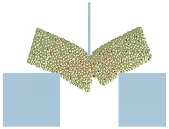
Figure 6.
The bending test of the cylindrical samples used in the EDEM.
It can be seen from the results that the error in the damage force in the physical test and simulation is less than 5%, and the destructive force has a good linear relationship with the diameter of the sample, indicating that the parameter calibration method was credible.
4. Conclusions
(1) The Poisson’s ratio and shear modulus of walnut kernels were determined by the compression test, and were 0.40 ± 0.26 and 1.87 ± 0.15 MPa, respectively.
(2) The friction between walnut kernels, the friction between the walnut kernel and the steel, the coefficient of elasticity of walnut kernels, and the elastic recovery coefficient between the walnut kernel and the steel plate were 0.8, 0.05, 0.3, and 0.7, respectively.
(3) After the two-level factor test, the steepest ascent test, and the response surface test, the repose angle of walnut kernels was determined by the quadratic equation and it was 37.35 ± 2.32°.
(4) Based on the bending test, the normal phase stiffness and tangential stiffness of walnut kernels were 1.72 × 10⁷, and 3.3 × 10⁶, respectively. The average destructive force was 32.5 N.
In this study, the DEM parameters required for the mechanized grading process of walnut kernels were determined. Subsequently, the bond fracture model of the walnut kernel was established by comparing the physical test and the simulation test. Meanwhile, it offers strong data support and technical support to design a grading machine for walnut kernels or for the analysis of the transport process of walnut kernels.
Author Contributions
Methodology, B.Z.; software, Y.Z.; validation, B.Z.; writing—original draft preparation, B.Z.; writing—review and editing, B.Z.; supervision, L.H.; project administration, L.H.; funding acquisition, L.H. All authors have read and agreed to the published version of the manuscript.
Funding
This work was supported by the National Key R&D Program of China (2018YFD0700105), and the Key Research and Development Program in Shaanxi Province of China (2023-YBNY-201).
Institutional Review Board Statement
Not applicable.
Data Availability Statement
Not applicable.
Conflicts of Interest
The authors declare no conflict of interest.
References
- Wang, S.; Yue, J.; Chen, B.; Tang, J. Treatment Design of Radio Frequency Heating Based on Insect Control and Product Quality. Postharvest Biol. Technol. 2008, 49, 417–423. [Google Scholar] [CrossRef]
- Di Pierro, E.; Franceschi, P.; Endrizzi, I.; Farneti, B.; Poles, L.; Masuero, D.; Khomenko, I.; Trenti, F.; Marrano, A.; Vrhovsek, U.; et al. Valorization of Traditional Italian Walnut (Juglans regia L.) Production: Genetic, Nutritional and Sensory Characterization of Locally Grown Varieties in the Trentino Region. Plants 2022, 11, 1986. [Google Scholar] [CrossRef] [PubMed]
- Liu, M.; Li, C.; Cao, C.; Wang, L.; Li, X.; Che, J.; Yang, H.; Zhang, X.; Zhao, H.; He, G.; et al. Walnut Fruit Processing Equipment: Academic Insights and Perspectives. Food Eng. Rev. 2021, 13, 822–857. [Google Scholar] [CrossRef]
- Monarca, D.; Cecchini, M.; Antonelli, D. Modern Machines for Walnut Harvesting. Acta Hortic. 2006, 705, 505–513. [Google Scholar] [CrossRef]
- Zhang, L.; Ma, H.; Wang, S. Pasteurization Mechanism of S. aureus ATCC 25923 in Walnut Shells Using Radio Frequency Energy at Lab Level. Lwt-Food Sci. Technol. 2021, 143, 111129. [Google Scholar] [CrossRef]
- Jiang, L.; Zhu, B.; Jing, H.; Chen, X.; Rao, X.; Tao, Y. Gaussian Mixture Model-based Walnut Shell and Meat Classification in Hyperspectral Fluorescence Imagery. Trans. ASABE 2007, 50, 153–160. [Google Scholar] [CrossRef]
- Zuo, Y.; Zhou, B.; Wang, S.; Hou, L. Heating Uniformity in Radio Frequency Treated Walnut Kernels with Different Size and Density. Innov. Food Sci. Emerg. 2022, 75, 102899. [Google Scholar] [CrossRef]
- Wang, Y.; Svetlana, A.; Yuriy, S. Evaluating the Efficiency of the Classifier Method When Analysing the Sales Data of Agricultural Products. Asian J. Water Environ. 2022, 19, 41–46. [Google Scholar] [CrossRef]
- Brawner, S.; Warmund, M. Husk Softening and Kernel Characteristics of Three Black Walnut Cultivars at Successive Harvest Dates. Hortscience 2008, 43, 691–695. [Google Scholar] [CrossRef]
- Prabhakar, H.; Kerr, W.; Bock, C.; Kong, F. Effect of Relative Humidity, Storage Days, and Packaging on Pecan Kernel Texture: Analyses and Modeling. J. Texture Stud. 2022. [Google Scholar] [CrossRef] [PubMed]
- Pakrah, S.; Rahemi, M.; Haghjooyan, R.; Nabipour, R.; Kakavand, F.; Zahedzadeh, F.; Vahdati, K. Comparing Physical and Biochemical Properties of Dried and Fresh Kernels of Persian Walnut. Erwerbs-Obstbau 2022, 64, 455–462. [Google Scholar] [CrossRef]
- Sugirbay, A.; Hu, G.; Chen, J.; Mustafin, Z.; Muratkhan, M.; Iskakov, R.; Chen, Y.; Zhang, S.; Bu, L.; Dulatbay, Y.; et al. A Study on the Calibration of Wheat Seed Interaction Properties Based on the Discrete Element Method. Agriculture 2022, 12, 1497. [Google Scholar] [CrossRef]
- Liu, Y.; Mi, G. Determination of Discrete Element Modelling Parameters of Adzuki Bean Seeds. Agriculture 2022, 12, 626. [Google Scholar] [CrossRef]
- Kotwaliwale, N.; Brusewitz, G.; Weckler, P. Physical Characteristics of Pecan Components: Effect of Cultivar and Relative Humidity. Trans. ASABE 2004, 47, 227–231. [Google Scholar] [CrossRef]
- Yu, Y.; Li, L.; Zhao, J.; Wang, X. Discrete Element Simulation Based on Elastic–plastic Damping Model of Corn Kernel–cob Bonding Force for Rotation Speed Optimization of Threshing Component. Processes 2021, 9, 1410. [Google Scholar] [CrossRef]
- Keppler, I.; Safranyik, F.; Oldal, I. Shear Test as Calibration Experiment for DEM Simulations: A Sensitivity Study. Eng. Comput. 2016, 33, 742–758. [Google Scholar] [CrossRef]
- Imole, O.; Krijgsman, D.; Weinhart, T.; Magnanimo, V.; Montes, B.; Ramaioli, M.; Luding, S. Experiments and Discrete Element Simulation of the Dosing of Cohesive Powders in a Simplified Geometry. Powder Technol. 2016, 287, 108–120. [Google Scholar] [CrossRef]
- Wu, J.; Collop, A.; McDowell, G. Discrete Element Modeling of Constant Strain Rate Compression Tests on Idealized Asphalt Mixture. J. Mater. Civ. Eng. 2011, 23, 2–11. [Google Scholar] [CrossRef]
- Chen, Z.; Xie, C.; Chen, Y.; Wang, M. Bonding Strength Effects in Hydro-mechanical Coupling Transport in Granular Porous Media by Pore-scale Modeling. Computation 2016, 4, 15. [Google Scholar] [CrossRef]
- Ren, J.; Wu, T.; Mo, W.; Li, K.; Hu, P.; Xu, F.; Liu, Q. Discrete Element Simulation Modeling Method and Parameters Calibration of Sugarcane Leaves. Agronomy 2022, 12, 1796. [Google Scholar] [CrossRef]
- Deng, P.; Liu, Q.; Huang, X.; Bo, Y.; Liu, Q.; Li, W. Sensitivity Analysis of Fracture Energies for the Combined Finite-Discrete Element Method (FDEM). Eng. Fract. Mech. 2021, 251, 107793. [Google Scholar] [CrossRef]
- Mi, G.; Liu, Y.; Wang, T.; Dong, J.; Zhang, S.; Li, Q.; Chen, K.; Huang, Y. Measurement of Physical Properties of Sorghum Seeds and Calibration of Discrete Element Modeling Parameters. Agriculture 2022, 12, 681. [Google Scholar] [CrossRef]
- Wang, S.; Chen, G.; Zhang, L. Parameter Inversion and Microscopic Damage Research on Discrete Element Model of Cement-stabilized Steel Slag Based on 3D Scanning Technology. J. Hazard. Mater. 2022, 424, 127402. [Google Scholar] [CrossRef] [PubMed]
- Li, H.; Zeng, R.; Niu, Z.; Zhang, J. A Calibration Method for Contact Parameters of Maize Kernels Based on the Discrete Element Method. Agriculture 2022, 12, 664. [Google Scholar] [CrossRef]
- Wang, Y.; Zhang, Y.; Yang, Y.; Zhao, H.; Yang, C.; He, Y.; Wang, K.; Liu, D.; Xu, H. Discrete Element Modelling of Citrus Fruit Stalks and its Verification. Biosyst. Eng. 2020, 200, 400–411. [Google Scholar] [CrossRef]
- Yu, Y.; Ren, S.; Li, J.; Chang, J.; Yu, S.; Sun, C.; Chen, T. Calibration and Testing of Discrete Element Modeling Parameters for Fresh Goji Berries. Appl. Sci. 2022, 12, 11629. [Google Scholar] [CrossRef]


Disclaimer/Publisher’s Note: The statements, opinions and data contained in all publications are solely those of the individual author(s) and contributor(s) and not of MDPI and/or the editor(s). MDPI and/or the editor(s) disclaim responsibility for any injury to people or property resulting from any ideas, methods, instructions or products referred to in the content. |
© 2023 by the authors. Licensee MDPI, Basel, Switzerland. This article is an open access article distributed under the terms and conditions of the Creative Commons Attribution (CC BY) license (https://creativecommons.org/licenses/by/4.0/).