Abstract
The prediction of the maturity date of leafy greens in a planting environment is an essential research direction of precision agriculture. Real-time detection of crop growth status and prediction of its maturity for harvesting is of great significance for improving the management of greenhouse crops and improving the quality and efficiency of the greenhouse planting industry. The development of image processing technology provides great help for real-time monitoring of crop growth. However, image processing technology can only obtain the representation information of leafy greens, and it is difficult to describe the causal mechanism of environmental factors affecting crop growth. Therefore, a framework combining an image processing model and a crop growth model based on causal inference was proposed to predict the maturity of leafy greens. In this paper, a deep convolutional neural network was used to classify the growth stages of leafy greens. Then, since some environmental factors have causal effects on the growth rate of leafy greens, the causal effects of various environmental factors on the growth of leafy greens are obtained according to the data recorded by environmental sensors in the greenhouse, and the prediction results of the maturity of leafy greens in the study area are obtained by combining image data. The experiments showed that the root mean square error (RMSE) was 2.49 days, which demonstrated that the method had substantial feasibility in predicting the maturity for harvesting and effectively solved the limitations of poor timeliness of prediction. This model has great application potential in predicting crop maturity in greenhouses.
1. Introduction
In Shanghai, leafy greens are usually planted in greenhouses. Although traditional planting technology is relatively mature, they have gradually become unable to meet the demand with the aging of the population and the growth of the demand for leafy greens. People began to apply automation and intelligent management technology to agricultural production so that labor shortages can be alleviated while improving crop quality.
The maturity of leafy greens is the key to affecting their yield and quality. Early or late harvest is not conducive to the income increase in leafy greens [1]. In the sense of agronomy, maturity refers to the stage when the nutrient storage organs of crops grow to harvest. The early method of maturity prediction is mainly a manual approach to predicting maturity by observing the crop growth state at fixed points on the ground [2], but it requires a lot of labor and time and has great limitations. In recent years, with the development of information technology and statistical science, different methods have been developed based on the factors affecting the changes in maturity and the changes in crop biochemical parameters. The first is the meteorological statistical model, which studies the influence of temperature, photoperiod, precipitation, and other factors on crops through the statistical analysis of historical data to achieve the prediction of crop maturity and summarizes the phenological development of a specific crop in a specific region, of which the growth degree day (GDD) is the most representative. Aslam et al. [3] showed that wheat flowering and maturity dates predicted by GDD are consistent with the observed data through two years of field experiments. Liu et al. [4] combined the traditional GDD algorithm with the artificial intelligence algorithm to predict the maturity of rice. Duan et al. [5] established a look-up table based on the meteorological data for many years and the crop maturity data of a certain year and believed that the more similar the climate conditions are, the closer the crop maturity will be. The other method is to extract the maturity period by analyzing the change characteristics of crop biochemical parameters during the growth period. This method mostly uses remote sensing data as the data source. Sakamoto et al. [6] established a two-step filtration (TSF) method for monitoring maize and soybean phenology by combining a day in a year with a wide dynamic range VI (WDRVI). Most of the existing forecasting methods based on environmental data are based on studies of the correlation between environmental factors and crop maturity. For example, Friis et al. [7] selected air temperature and soil temperature as prediction variables, conducted regression analysis in stages, and finally constructed a prediction model of pea maturity, realizing the prediction of pea maturity. These methods all have great fitting effects, but the models of which are essentially fitting means for observation data, and it is difficult to explain the causal mechanism of environmental factors affecting crop growth through these models. Correlation does not necessarily imply causality, but causality generally leads to correlation at the statistical level. If we combine causality and correlation modeling together, theoretically, the performance of the model will be better than using correlation modeling only, and the model will become more interpretative and robust.
The above research mainly analyzes historical data to predict the maturity of a large area. The prediction of crop maturity in a greenhouse environment has a higher demand for precision agriculture and requires short-term prediction of crop maturity [8], which means we need to predict the maturity date day-by-day throughout the leafy greens’ growth cycle. In recent years, with the development of imaging technology and computer vision technology, crop maturity prediction based on images has gradually become a hot research topic. Previous studies used image technology to predict crop maturity, mainly through spectral information prediction [9], electronic nose, electronic tongue [10] combined with partial least squares regression analysis, and color eigenvalue combined with back-propagation neural network [11]. When the internal mechanism and relationship are uncertain, backpropagation neural networks (BPNNs) [12] are considered a model with high accuracy. Among these methods, BPNNs are multilayer neural networks that can be trained according to error backpropagation, and are the most widely used neural networks. BPNNs can be used to consider the interaction between inputs and outputs, improve the prediction accuracy, and is more effective than traditional discriminant analysis and multiple logistic regression regions [13]. Most relevant studies use BPNNs for function approximation, regression analysis, numerical prediction, classification, and data processing [14]. In previous studies, researchers mainly focused on field crops, greenhouse fruits, and other crop varieties. For example, Xuan et al. [15] used Vis/NIR hyperspectral imaging technology to evaluate the maturity of green bananas. However, there are few studies focusing on leafy greens in the greenhouse. Therefore, this paper will take leafy greens planted in the greenhouse as the research object, adopt causal inference as the main research method of crop growth model, fuse image classification algorithm to process the image data of leafy greens, and use the optimized prediction model to predict the maturity of regional leafy greens.
2. Study Area and Materials
2.1. Study Area
A leafy green planting base in Shanghai is selected as the research area. It is centered at 31.14 degrees North latitude and 121.29 degrees East longitude and the front of the Yangtze River Delta on the west coast of the Pacific Ocean. It has a subtropical oceanic monsoon climate, with an average annual precipitation of about 1056 mm and an average temperature of 15.5 °C. Leafy greens are one of the main crops grown in this area. Leafy greens can be sown throughout the year since the greenhouse keeps the environment warm. However, due to the differences in meteorological conditions and sowing time, the maturity date of leafy greens in different batches in the study area also has certain differences.
2.2. Research Data
2.2.1. Image Data of Leafy Greens
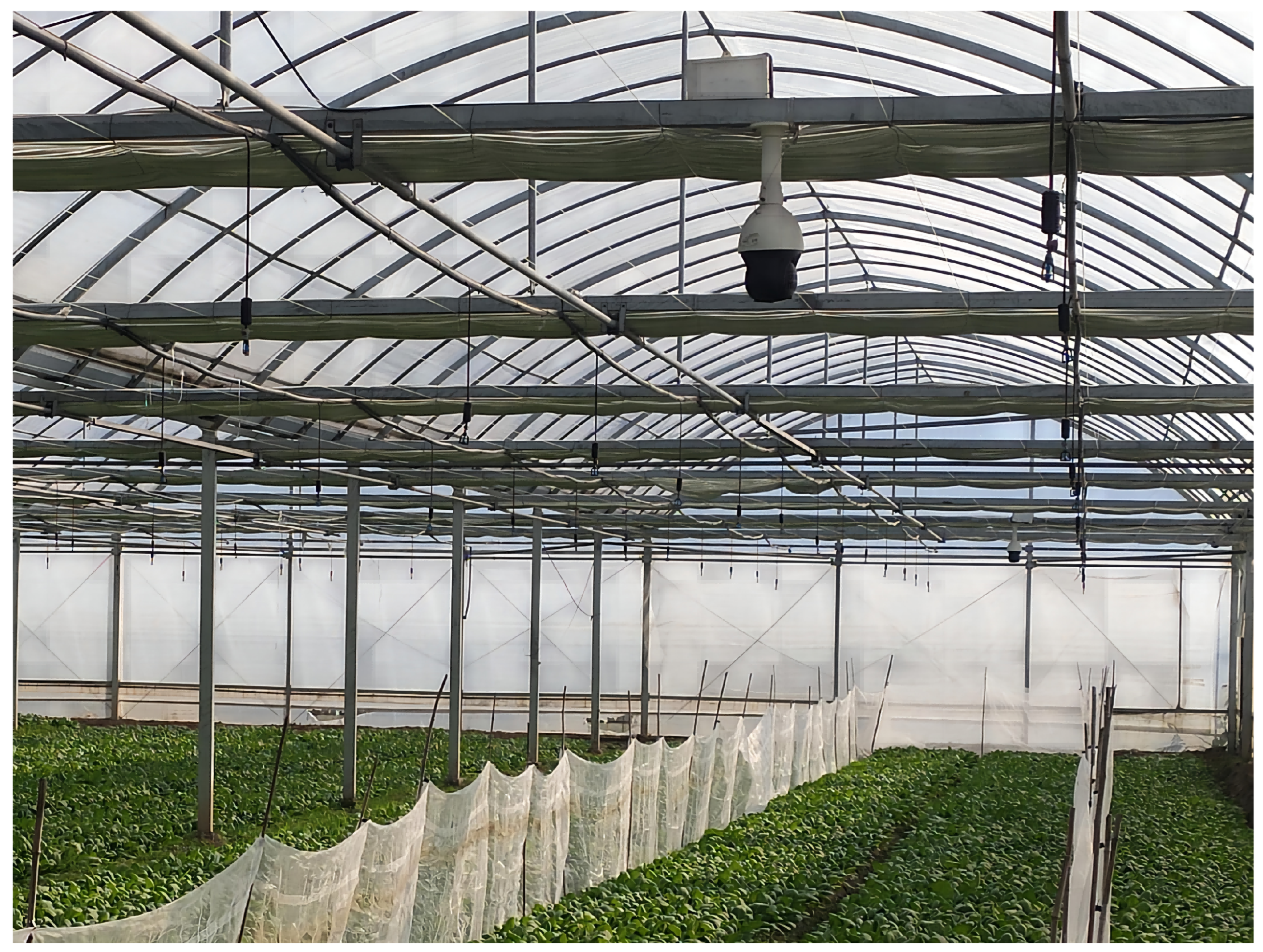
In order to train the depth convolution neural network and verify the algorithm proposed in this paper, we collected image data in the greenhouse of the area described in Section 2.1. In order to photograph the leafy greens in the same area for multiple days, several fixed cameras were installed on the top shelf of the greenhouse. The installation of the greenhouse camera is shown in Figure 1.
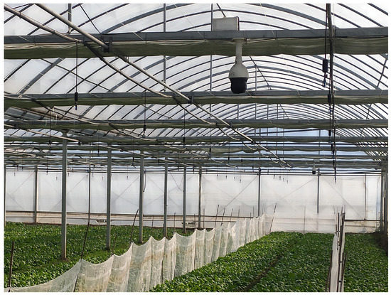
Figure 1.
Installation of the camera in the greenhouse.
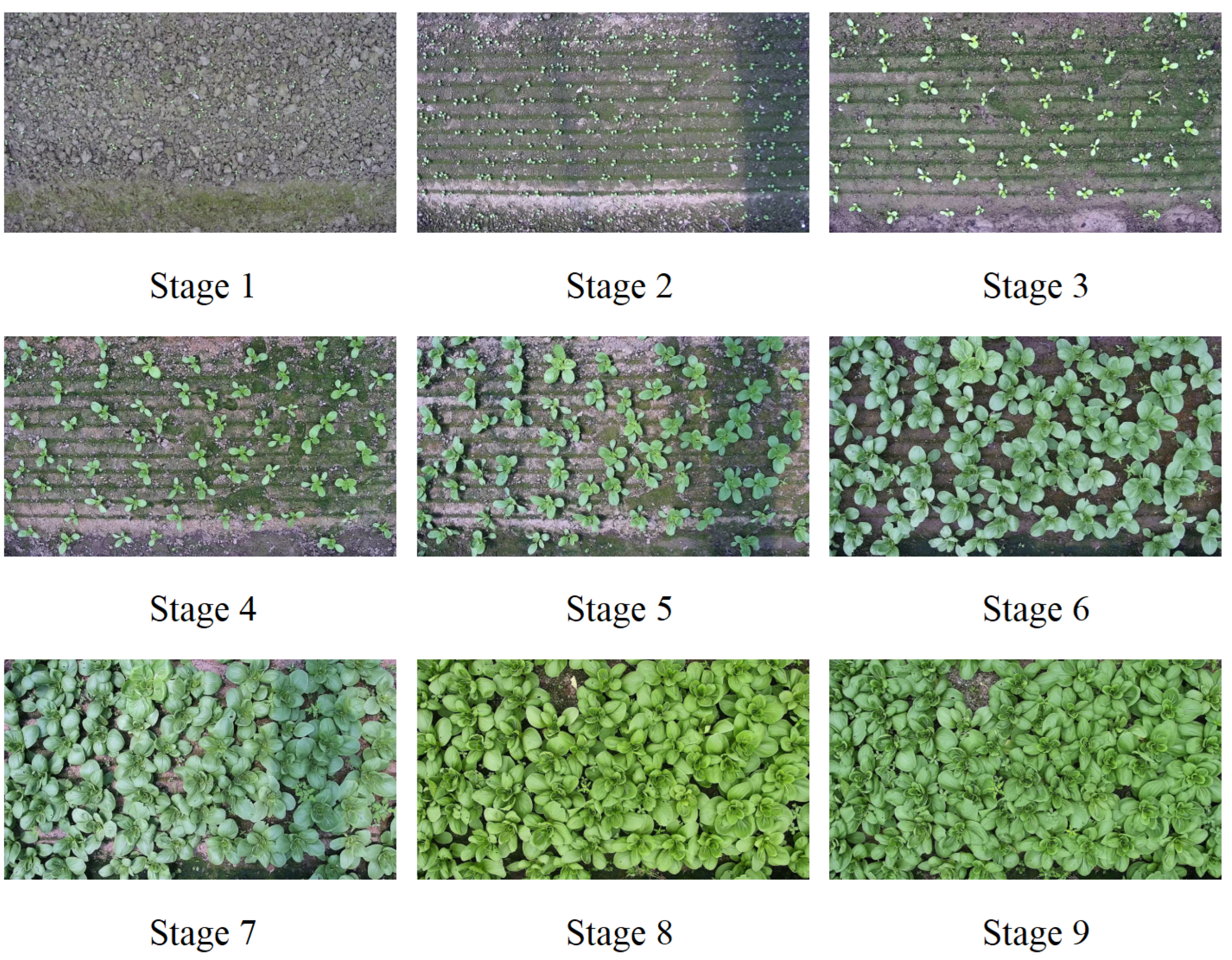
A total of 362 images with a resolution of 1920 × 1080 px were collected, including the morphological changes of leafy greens from bud to maturity. Taking the growth cycle of the fastest-growing green leafy vegetables, for example, which were sown in spring. Based on different forms of leafy greens, we divided them into nine growth stages at an interval of 4 days and classified them as categories, as shown in Figure 2. All images were manually labeled based on the photography date and the morphological characteristics of leafy greens and used as a data set. Finally, the data set was divided into the training set, verification set, and testing set at a 3:1:1 ratio.
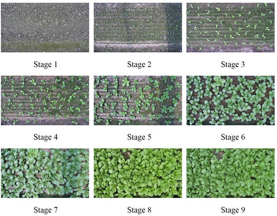
Figure 2.
Images of leafy greens in different growth stages.
2.2.2. Agricultural Environmental Data
The greenhouse environment is a typical complex system. In order to find accurate causal effects, a set of accurate and reliable sensor systems is essential. The greenhouse for planting leafy greens adopts the sensor equipment of Zuoan Xinhui Company, which adopts RS485 communication mode. The data collected by the sensor network include: indoor temperature, indoor humidity, indoor light intensity, soil temperature, soil humidity, soil PH value, and soil EC value. Table 1 lists the sensors used and the environmental factors collected. The data used in this paper starts from 14 April 2021, and the data deadline is 21 May 2022. Each sensor records data every 10 min and sends it back to the database. We average these environmental data in daily units, and then the accuracy of the prediction model is also in daily units.

Table 1.
List of sensors used by the system.
3. Methods
As introduced in Section 1, the maturity prediction of leafy greens requires taking into account the current growth status of leafy greens and the environmental information in the greenhouse. In order to determine the current growth state of leafy greens, this paper implements the classification task of leafy greens based on a deep neural network. The attention mechanism is added to capture the salient features of images in different growth stages of leafy greens and improves the feature extraction ability of a convolution neural network. This approach will be described in detail in Section 3.1.
In order to obtain a causal effect prediction model based on environmental data, including soil parameters, this paper uses the method of causal inference to obtain the causal effects of various environmental characteristics on the growth state of leafy greens. Combined with the real-time information recorded by environmental sensors, the prediction results are optimized. This approach will be described in detail in Section 3.2. Considering the impact of historical environmental information on the crops and the robustness of the model, in this paper, we combine the image processing module, causal effect estimation model, and the historical prediction information to obtain the prediction results of the mature date of leafy greens in the greenhouse. This approach will be described in detail in Section 3.3.
3.1. Image Classification Module
In order to obtain the growth state of leafy greens and infer their maturity date, this paper analyzes the phenotype of leafy greens based on a deep convolution neural network to determine their growth stage. In the field of computer vision, the technology of object detection and instance segmentation is relatively mature. A naive idea is to calculate the average leaf area of leafy greens by case segmentation and compare the growth curve to determine its growth stage. However, in the actual planting environment, the planting of leafy greens is crowded, and the occlusion between vegetable leaves is very serious, so the effect of this kind of model is not good. Considering that the color, texture, and other different features of leafy greens can also be used to judge their growth stages, this paper directly uses image classification algorithms to classify the collected leafy greens images.
When a convolutional neural network classifies leafy greens images, it mainly relies on convolutional layers to extract the features of images at different growth stages. Given the input image, the convolutional neural network performs image preprocessing, feature extraction and classification and finally outputs the label of the prediction category. Among them, the most critical step is extracting the effective feature information. Common convolutional neural network models for phenotypic analysis of crops include VGGNet [16], Inception V3 [17], ResNet34 [18], etc. ResNet [19] effectively solves the phenomenon of gradient disappearance in neural network training by introducing a residual module. In this paper, we adopt a 34-layer ResNet network, which is composed of a series of residual modules, a full connection layer, and a lower sampling layer, as shown in Figure 3.
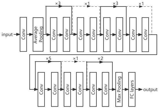
Figure 3.
Network structure of ResNet34.
The parameters in ResNet are gradually updated by comparing the error between the predicted value of the model and the ground truth, and the loss function is used to measure the degree of inconsistency between the predicted value and the true value. In this paper, in order to predict the growth stage of leafy greens, the final loss function value is calculated using the cross-entropy function, which is a weighted average of the cross-entropy of each sample in the input network, and the specific calculation formula is
where represents the ground truth of sample i in class j, represents the prediction probability of sample i on class j, and n is the number of samples.
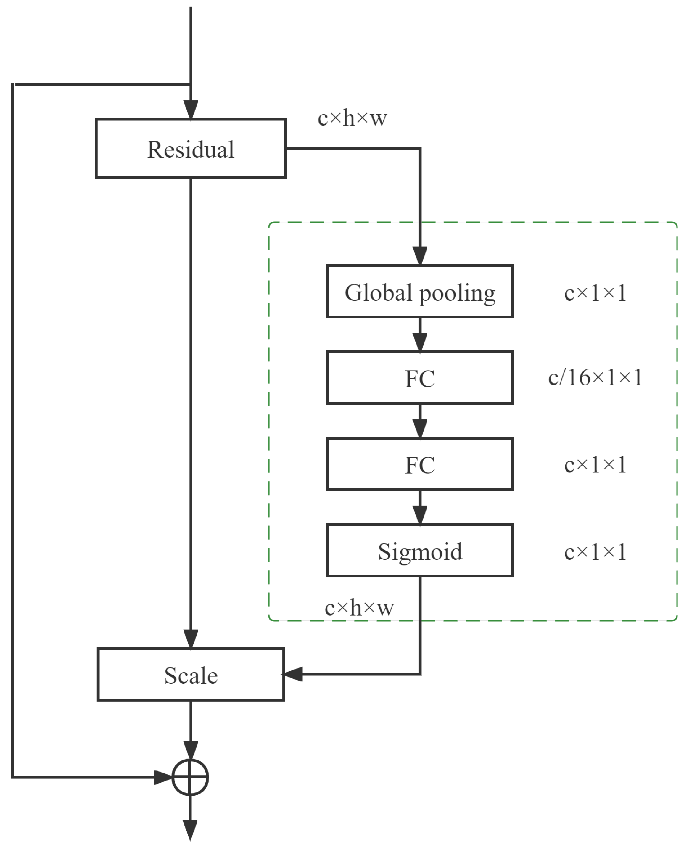
In the classification task of leafy greens planted in the greenhouse, the prediction results are easily affected by soil and weeds, and our expected algorithm is to focus on the characterization of leafy greens. Therefore, the attention mechanism is introduced in this paper. By embedding the existing SE channel attention mechanism [20] into the end of each residual structure of the original ResNet network, the network feature extraction ability is improved to capture significant feature information, such as shape, color, etc., on the leafy greens image. The basic module of SENet attention and residual network integration is shown in Figure 4. Specifically, we adopt the network structure of Global Average pooling-FC-Relu-FC-Sigmoid. SENet has two fully connected (FC) layers, and the two functions are opposite. First, the FC layer of the first layer will reduce the number of channels in the network. On the contrary, the FC layer of the second layer will increase the number of channels. The weight will be generated in this process, and the weight is equal to the number of channels, which can still provide the weight value for the corresponding channel. The core of SENet is to use the loss of the network to understand the weight of the features and assign a larger weight to efficient feature graphs and a smaller weight to useless or less-efficient feature graphs so as to train the model and obtain better results. In general, the SE channel attention mechanism reduces the error rate of the previous model to a large extent, and the new parameters and calculation amount are small. Therefore, we add this attention mechanism to the ResNet network.
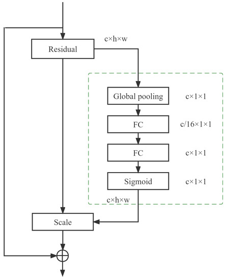
Figure 4.
Residual networks under SENet attention mechanism.
3.2. Causal Effect Estimation Model of Environmental Factors
Crop growth is closely related to its environment, so the role of environmental factors should be considered when predicting the maturity date of leafy greens. At present, most studies predict the maturity date by building crop growth models based on environmental factors such as temperature and light. These methods have some limitations; not only the selection of environmental variables is limited, but also the multicollinearity and causal relationship between variables are ignored. In this paper, the causal inference technology is used to find the causal relationship between environmental factors in the greenhouse and the growth rate of leafy greens. On the one hand, the accuracy of the model prediction is improved. On the other hand, the causal mechanism between environmental factors and the growth of leafy greens is analyzed to a certain extent, which is conducive to the accurate control of the greenhouse environment in the future. Causal inference has achieved fruitful results in econometrics, sociology, computer science, and other fields [21,22,23]. Since this is a new research direction and is limited by the collection and analysis of data, causal inference technology has less application in the field of agriculture and still has great potential.
Causal inference usually refers to the search for causality, while causality refers to the relationship between one event (i.e., “cause”) and another event (i.e., “effect”), in which the latter event is considered the outcome of the previous event. Generally speaking, causality can also refer to the relationship between a series of factors (causes) and a phenomenon (effect). Any event that affects the outcome is a factor in the outcome [24]. It is generally recognized that the most effective causal inference method is random controlled trials (RCT). However, it is often inoperable, and its scope of the experiment cannot cover all real scenes. Therefore, we consider the causal inference method based on observation data. At present, the mainstream causal analysis methods based on observational data are mainly divided into two categories: a potential consequence model and the structural causal model. Among them, the potential outcome model constructs a new analytical framework for causal inference by drawing on the concepts of randomized controlled trials and potential outcomes in statistics. Compared with the potential outcome model algorithm, the structural causal model is used to find the causal relationship between multiple variables. Based on Bayesian networks, Pearl [25] proposed the concept of intervention and expressed causality in a formal way, which pioneered the method of extracting causality and the data generation mechanism from data.
According to the data characteristics of various environmental factors in a greenhouse planting environment, this paper adopts the methods of potential outcome model and structural causal model for different environmental factors and calculates the causal effect by observing the length of the growth cycle of leafy greens in different environments.
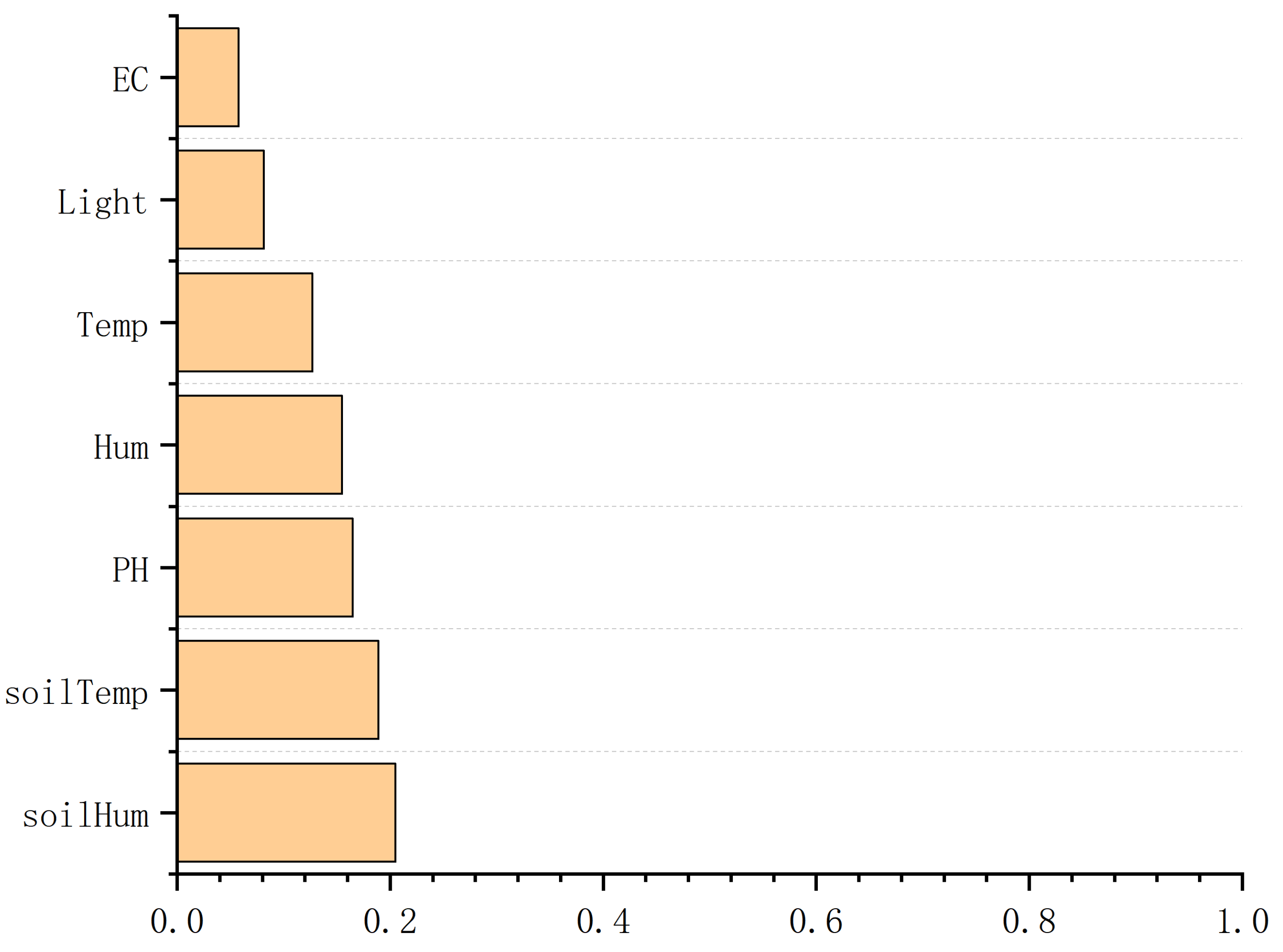
First, we mine and collect causal environment variables and then use xgboost [26] to detect the correlation between input variables and outcome variables, including whether there is a correlation and the strength of the correlation. Seven variables are used to rank the importance of features, as shown in Figure 5.
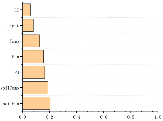
Figure 5.
Analysis chart of the importance of environmental factors.
After confirmation with greenhouse planting professionals, these variables with obvious correlation are basically consistent with empirical judgment. Based on the data distribution characteristics and empirical judgment, we treat soil temperature as a continuous variable to calculate its continuous causal effect on the growth of leafy greens, and other environmental factors are regarded as binary variables to calculate relatively rough causal effects. We use graph theory as a mathematical tool to formalize the causal hypothesis behind the leafy green growth model, infer the causal relationship of environmental factors other than soil temperature through the structural causal model, and calculate the more accurate causal effect of soil temperature through the nonlinear model.
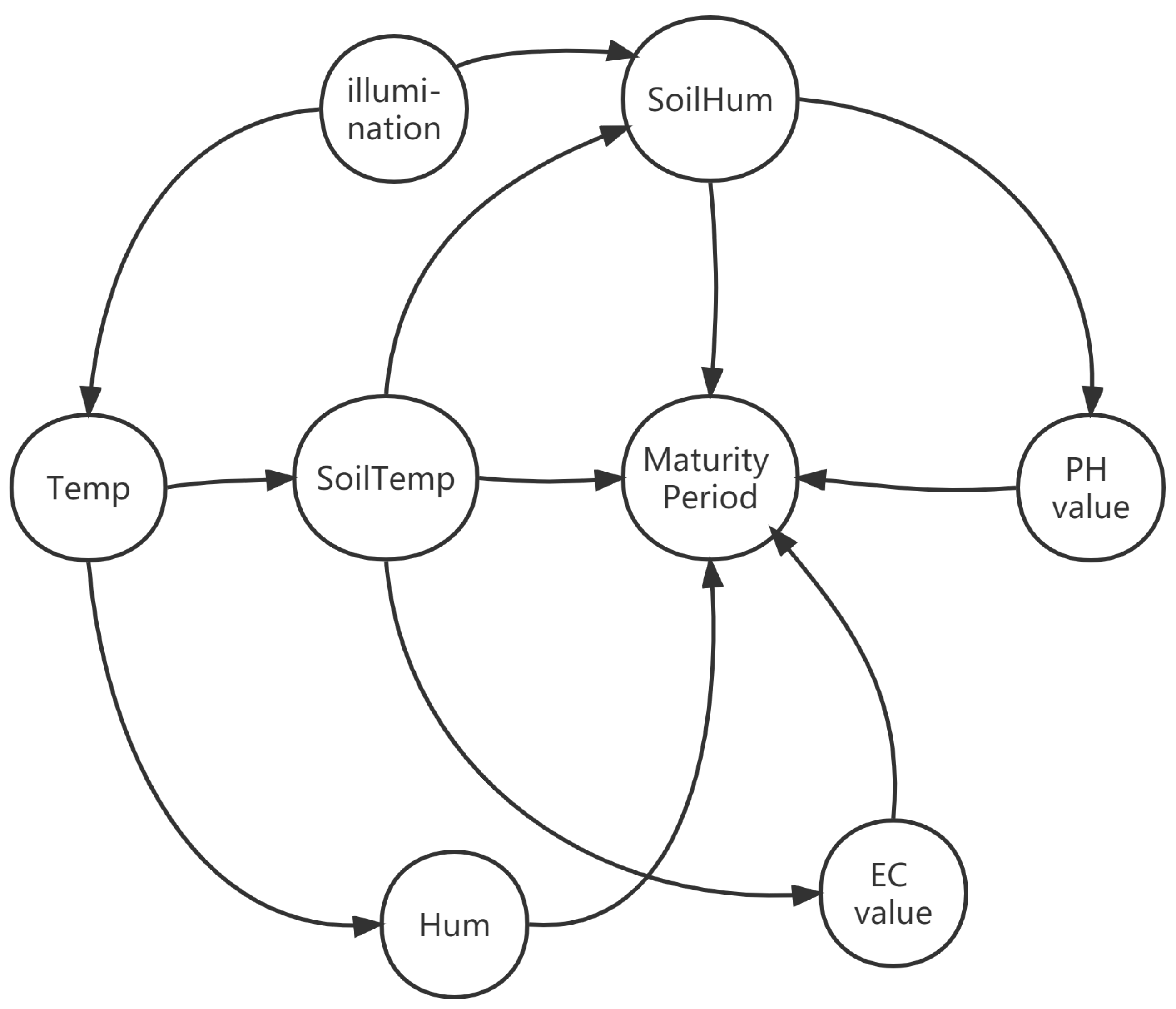
The structural causal model adopted in this paper is based on directed acyclic graphs (DAGs) [25]. Therefore, the causal diagram is established based on the PC algorithm [27] and prior knowledge of the relationship between environmental factors and crop growth [28], as shown in Figure 6.

Figure 6.
Causal diagram of environment and leafy greens.
The graph model provides a visual representation of causality, and joint distribution can be obtained by statistical analysis of observed data, but it is difficult to identify causality from these correlations. Therefore, we need to intervene, which means changing the existing data distribution to identify causality. Pearl [25] proposed to express intervention with do-calculus, and the variables to be studied were X and Y, the vector composed of other covariates is . For simplification, suppose X is a binary variable; that is, the value can only be 0 or 1. A set of data is observed. For example, represents the probability distribution of under the condition of . represents the probability distribution of when is achieved through intervention. Because of the existence of confounders, usually , in order to analyze the causal effects of pairs in the causal model, we need to adjust for all confounders. For example, confounders can be removed through backdoor adjustment. Given a pair of ordered variables in the model, if there is no descendant of X in confounder set Z and all backdoor paths between X and Y are blocked by confounder set Z, then confounder set Z meets the backdoor adjustment, and backdoor paths pointing to X can be blocked to find the causal effect, as shown in the following formula
If all the elements of the blocking path are unobservable, the backdoor path cannot be calculated. However, if all the paths from X and Y have elements z, and there is no open path from z to Y, we can use the set Z of z to measure , i.e., the frontdoor adjustment. The following formula converts the expression containing do-calculus into the expression without do-calculus by taking the variable set Z on the frontdoor path as a condition:
Using the backdoor adjustment and the frontdoor adjustment to intervene the causal diagram with the elimination of the do-calculus, the causal relationship between variables can be inferred only through known observation data and variable distribution. After identifying the causality between each node on the causal diagram of environment and leafy greens, we estimate the causal effect, that is, use the historical data recorded by greenhouse environmental sensors to calculate the specific value of the causal effect. First, the causal effect of environmental factors other than soil temperature is calculated by using propensity score matching (PSM) [29]. Since we set these environmental factors as binary variables, the treatment for each environmental factor is binary, and the treatment . Then our outcome is the growth cycle y of leafy greens. In addition, feature X is composed of each environmental factor, where represents the feature vector of sample i. Our goal is to estimate the causal effect of t on y, called the average treatment effect (ATE)
where represents the individual treatment effect (ITE) and is defined as .
For PSM, it must find an object for each instance. It assumes that treatment t is a random variable extracted from a certain distribution, i.e., , and then a propensity score will be calculated. This propensity score is to calculate the given x. It tends to receive the probability of a certain treatment, that is, a binary score. Generally, this score is fitted with LR. After obtaining the propensity score, we will find an object different from its treatment for each sample. Therefore, for sample i, we find sample j s.t . The obtained ATE is
As the environmental factor that has the greatest impact on the maturity of leafy greens, we regard soil temperature as a continuous variable and take 2 °C as an interval to calculate the continuous treatment effect. The double machine learning (DML) [30] method is used to realize the unbiased estimation of the influence of the target on the feature. The random forest algorithm is used to fit Y and T, respectively, and each fitting is combined to obtain the residual.
where and are the fitted residuals. After we get the residual model, treatment effect can be obtained by fitting a simple regression model . In fact, the residual is the change quantity, so is the description of the relationship between the two residual quantities, that is, the causal effect ATE. is an equation related to X. We can solve it by the least square method.
3.3. Prediction Model of Leafy Greens Maturity Date
The prediction model of greenhouse leafy greens maturity date proposed in this paper combines the phenotypic characteristics of leafy greens and environmental factor data to achieve real-time short-term prediction of leafy greens, as shown in Figure 7.
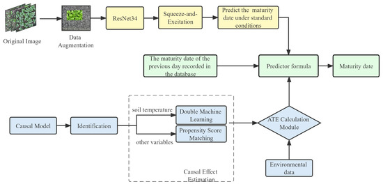
Figure 7.
Block diagram of the proposed prediction model.
First, the growth stage of leafy greens on that day can be judged by the image classification model introduced in Section 3.1. According to the growth stage, the maturity date of leafy greens in the standard environment can be inferred. Then, the causal inference model introduced in Section 3.2 is used to calculate the inhibition or promotion of each environmental factor on the growth of leafy greens on that day so as to adjust the predicted maturity date. Considering that the classification results of the model have errors and historical information can increase the robustness of the model, the prediction model also combines the historical predicted date in the database, and the final predicted maturity date is
where and are the weight of the historical forecast date and the current forecast date, which are hyperparameters, and . i represents the environmental factor.
4. Results
4.1. Results of Image Classification
The deep neural network is implemented by PyTorch framework. The specific test environment is shown in Table 2.
Table 2.
Experimental environment.
The image classification model described in Section 3.1 is trained using the following configuration. In the training phase, the following hyperparameters are selected for optimization: the optimizer is SGD; the number of training steps is 300; the batch size is 4; the learning rate is 0.01. In this paper, Top-1 Acc refers to taking the largest component in the probability vector as the final prediction result, and the prediction result is the same as the ground truth. This paper uses ResNet-34 as a benchmark to compare the TOP-1 Acc of SE-ResNet embedded in the SE channel attention mechanism and the original ResNet on the leafy green dataset, and adds the data enhancement method of cutout [31] during training to improve the accuracy. The results are shown in Table 3. Compared with the original ResNet network, the accuracy of the ResNet model with the SE module has increased by 8.4%, indicating that its performance has been significantly improved. After adding data enhancement, the accuracy is further improved by 2.8%.
Table 3.
The results of image classification on the testing set.
4.2. Results of Causal Effect Estimation
According to the analysis in Section 3.2, we consider environmental factors other than soil temperature as binary variables. Therefore, the values of environmental data in the suitable range for the growth of leafy greens were set to 0, and the values of environmental factors outside these intervals were set to 1. The suitable range for the growth of leafy greens is shown in Table 4.
Table 4.
Suitable range of different environmental factors for the growth of leafy greens.
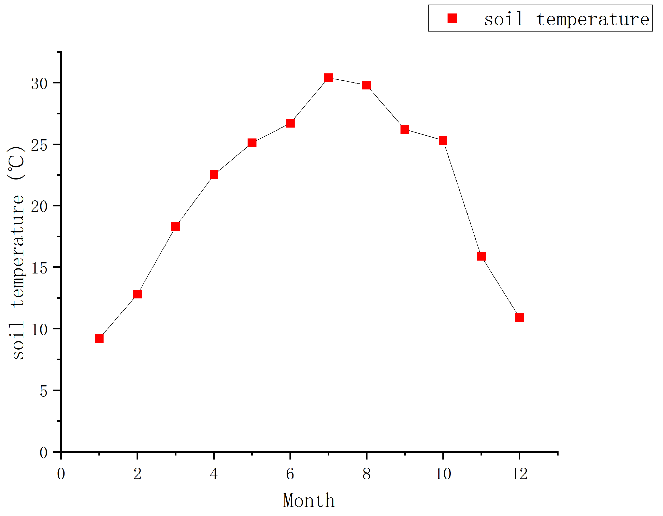
We calculate the continuous causal effect of soil temperature in a unit of 2 °C. Figure 8 describes the annual average temperature change in the greenhouse. Based on the observed data, we analyzed the causal effect of soil temperature in the range of 8–32 °C on the growth cycle of leafy greens.

Figure 8.
Annual average monthly temperature in the greenhouse where the experiment is conducted.
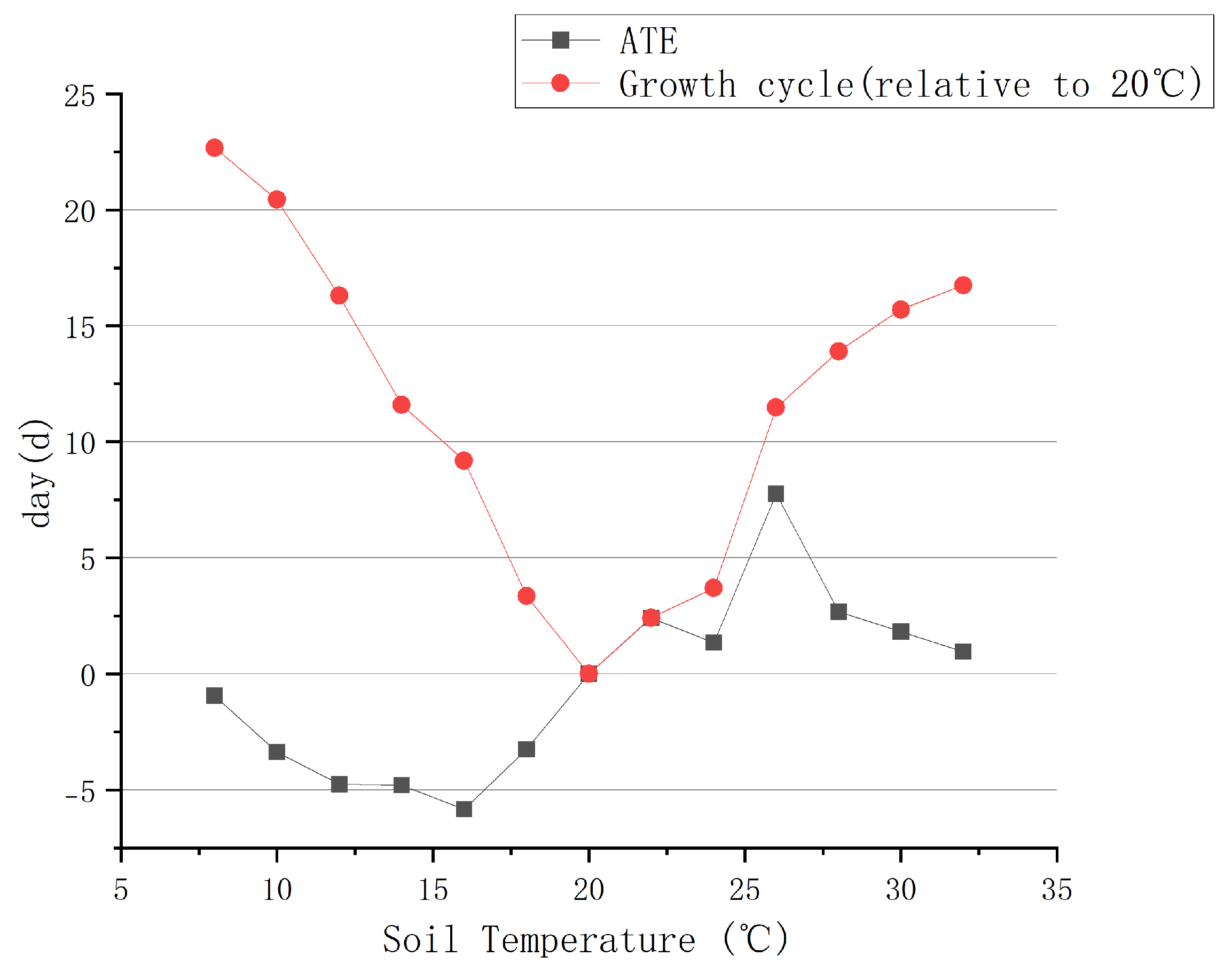
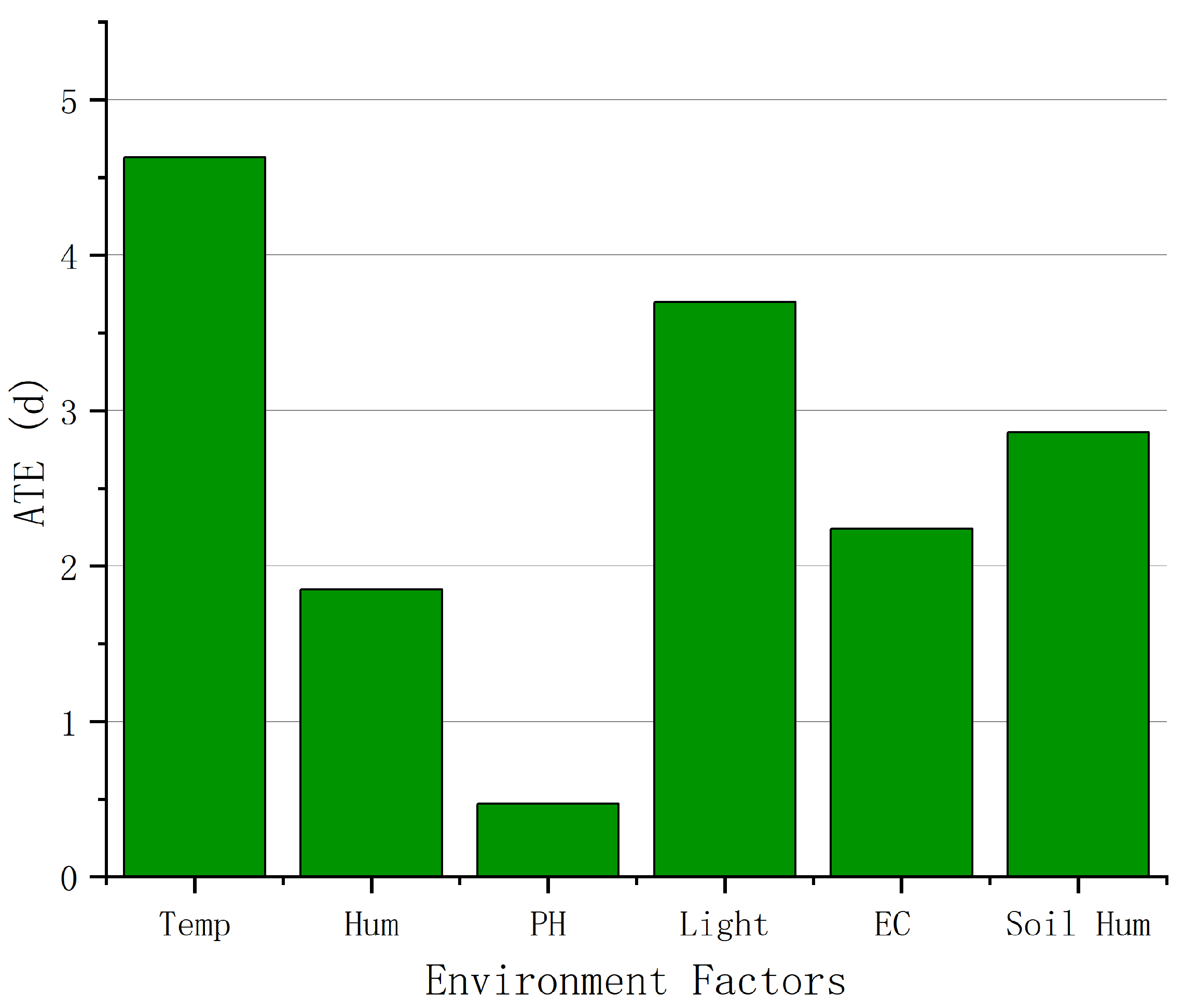
After filling in the missing values and data preprocessing, we used the DML algorithm and the PSM algorithm introduced in Section 3.2, respectively, to estimate the causal effects of soil temperature and other environmental factors on the growth cycle of leafy greens, as shown in Figure 9 and Figure 10, respectively. As a key factor affecting the maturity of leafy greens, the soil temperature is most suitable for the growth of leafy greens at about 20 °C. When the temperature increases or decreases, the growth cycle of leafy greens gradually becomes longer. When the temperature is about 8 °C, the growth inhibition of leafy greens is the most obvious, which is 22.67 days longer than that at 20 °C. In addition to soil temperature, indoor temperature and light also have obvious causal effects on the growth of leafy greens. Relatively speaking, the pH value has the weakest causal effect, with an ATE of less than 0.5 d.
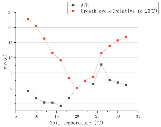
Figure 9.
The causal effect of different soil temperatures on the growth of leafy greens and the effect of relative 20 °C on the growth cycle.

Figure 10.
Causal effects of different environmental factors on the growth of leafy greens.
4.3. Results of Prediction Model
After adding the causal effects of different environmental factors obtained in Section 4.2, the prediction model proposed in Section 3.3 can realize the real-time prediction function of leafy greens maturity based on image data and environmental data. We selected untrained leafy green image sequences and their corresponding daily environmental data to predict the maturity of leafy greens. We start the prediction from the sprouting of leafy greens and add the historical prediction information from the next day, as shown in Formula (9) above, where and . The selected evaluation indicators are Mean Absolute Error (MAE) and Root Mean Square Error (RMSE). The prediction results of the model are shown in Table 5. Compared with the prediction model that only uses image features, the prediction result of the prediction model with causal inference has been significantly improved, and the RMSE has reached 3.15 d. Further analysis of the prediction accuracy of the model at different stages is shown in Table 6. It can be found that the RMSE of the model at the late growth stage of leafy greens is not only not improved but also slightly degraded compared with the early growth stage. This is contrary to common sense because the more mature the general prediction model is, the less difficult it is to predict, and the closer the results are. After analyzing the model, it is found that when the image classification module proposed in this paper judges the growth stage of leafy greens, the morphology of leafy greens in the later growth stage is relatively similar, and it is difficult to distinguish by the naked eye, so the classification effect is poor. For this reason, the hyperparameters of the model are slightly changed in the later stage, making the model more dependent on the historical prediction information recorded the previous day, reducing the importance of image classification models. According to the results in Table 7, we set as 0.8 and as 0.2 in the later stage. The RSME of the optimized model has been further improved, reaching 2.49 d, basically meeting the needs of modern agriculture.
Table 5.
The results of the prediction model.imgproc only uses the image classification module, +ATE combines the causal effect of environmental factors, and +ATE* adjusts the hyperparameters and .
Table 6.
Prediction results in different growth stages of leafy greens.
Table 7.
Results of prediction models under different hyperparameters at the late growth stage of leafy greens.
5. Discussion
In order to predict the maturity of leafy greens in greenhouse environments, it is necessary to consider multiple types of data. If only a single type of data is considered, the prediction results will be inaccurate and less robust. The phenotypic characteristics of leafy greens well reflect the growth state of leafy greens. In this paper, we use a deep convolutional neural network to judge the growth stage of leafy greens so as to preliminarily obtain the predicted maturity date under a standard environment. Compared with the image-based crop maturity prediction method [9,10,11,12], the model proposed in this paper requires fewer parameters to be set manually and is an end-to-end model with more accurate results. Table 3 shows that adding the attention mechanism to the classification model can effectively reduce background interference. At the same growth stage, leafy greens have similar phenotypic characteristics, but under different environmental conditions, their distance from the maturity date will be very different since environmental factors have causal effects on the growth of leafy greens. Therefore, we identified the causality in the growth environment of leafy greens and estimated the causal effect (ATE) based on the structural causal model. Compared with the previous prediction model considering environmental data [7], the model proposed in this paper takes into account the complex causal relationship between various environmental factors, which improves the model’s interpretability and prediction accuracy.
The method in this paper also has some limitations. (1) When leafy greens grow close to maturity, their phenotypic characteristics basically no longer change, so the image classification model is prone to errors, resulting in a slight decline in the final prediction results compared with the early growth period, as shown in Table 6. One solution is to increase the weight of historical prediction results in the late growth period of leafy greens and reduce the dependence of the prediction results on the image data taken on the same day. (2) When we build the causal diagram, we are mainly based on the experience of professional knowledge. At the same time, there are numerous hidden confounders in the real environment that we cannot observe. Therefore, errors may exist in the result when estimating the causal effect. In the future, the causal model can be optimized, and based on the results of real-time analysis of the causal model, the reasons affecting crop growth can be found so as to control the greenhouse environment to promote crop growth.
6. Conclusions
In this paper, a multifactor prediction model of leafy green maturity was established to predict the maturity date of leafy greens in a greenhouse. The environmental data in the greenhouse are selected as the variables of causality analysis, and the environmental sensor is used as the environmental data source. The images of leafy greens collected by the fixed camera are used as the input of the improved ResNet model, and the sowing date of leafy greens is used as the starting time of prediction to continuously predict the maturity of leafy greens. The conclusions of this research are as follows: (1) the predicted maturity dates after model fusion basically coincide with observation, and the RMSE is 2.49 days. Therefore, the framework can accurately predict the maturity of leafy greens. In addition, this framework uses the method of causal inference, which has strong interpretability and is more targeted for future work of regulating the greenhouse environment. (2) The model can predict the maturity date for harvesting leafy greens at the early stage of growth, and the prediction effect of the early and middle growth of leafy greens is ideal. However, due to the small changes in the phenotypic characteristics of leafy greens in the later growth period, the prediction results of the model are worse than expected. By adjusting the hyperparameters, the difficulty of image classification of leafy greens was solved to a certain extent.
In the future, the detailed effect of the prediction model for leafy greens maturity can be further optimized. In addition, the maturity date for the harvesting of leafy greens has a significant impact on their yield and quality, and reasonably promoting their ripening has certain economic benefits. Therefore, more tasks, such as greenhouse environmental control, can be implemented based on the causal inference model.
Author Contributions
Conceptualization, F.S.; Data curation, J.S. and X.H.; Funding acquisition, F.S. and X.H.; Methodology, J.S.; Project administration, F.S.; Software, J.S.; Supervision, F.S.; Visualization, J.S.; Writing—original draft, J.S.; Writing—review and editing, F.S. and X.H. All authors have read and agreed to the published version of the manuscript.
Funding
The research presented in this paper was supported in part by Shanghai Agriculture Applied Technology Development Program, China (Grant No. 2020-02-08-00-07-F01480).
Institutional Review Board Statement
Not applicable.
Data Availability Statement
Not applicable.
Conflicts of Interest
The authors declare no conflict of interest.
References
- Ierna, A. Influence of harvest date on nitrate contents of three potato varieties for off-season production. J. Food Compos. Anal. 2009, 22, 551–555. [Google Scholar]
- Zhang, M. Study on the Method of Crop Pehnology Detection and Crop Types Discrimination Based on MODIS Data. Ph.D. Thesis, Huazhong Agricultural University, Wuhan, China, 2006. [Google Scholar] [CrossRef]
- Aslam, M.A.; Ahmed, M.; Stöckle, C.O.; Higgins, S.S.; Hassan, F.U.; Hayat, R. Can growing degree days and photoperiod predict spring wheat phenology? Front. Environ. Sci. 2017, 5, 57. [Google Scholar]
- Liu, L.W.; Lu, C.T.; Wang, Y.M.; Lin, K.H.; Ma, X.; Lin, W.S. Rice (Oryza sativa L.) Growth Modeling Based on Growth Degree Day (GDD) and Artificial Intelligence Algorithms. Agriculture 2022, 12, 59. [Google Scholar] [CrossRef]
- Sheng, D.J. Effect of climate warming on mature date of winter wheat and forecast of harvest in Eastern Gansu Province. Agric. Res. Arid. Areas 2007, 25, 158–161. [Google Scholar]
- Sakamoto, T.; Wardlow, B.D.; Gitelson, A.A.; Verma, S.B.; Suyker, A.E.; Arkebauer, T.J. A two-step filtering approach for detecting maize and soybean phenology with time-series MODIS data. Remote Sens. Environ. 2010, 114, 2146–2159. [Google Scholar]
- Friis, E.; Jensen, J.; Mikkelsen, S. Predicting the date of harvest of vining peas by means of air and soil temperature sums and node countings. Field Crops Res. 1987, 16, 33–42. [Google Scholar] [CrossRef]
- Liu, L.; Zhang, X.; Yu, Y.; Guo, W. Real-time and short-term predictions of spring phenology in North America from VIIRS data. Remote Sens. Environ. 2017, 194, 89–99. [Google Scholar] [CrossRef]
- Nguyen, N.M.T.; Liou, N.S. Ripeness Evaluation of Achacha Fruit Using Hyperspectral Image Data. Agriculture 2022, 12, 2145. [Google Scholar] [CrossRef]
- Xu, S.; Li, J.; Baldwin, E.A.; Plotto, A.; Rosskopf, E.; Hong, J.C.; Bai, J. Electronic tongue discrimination of four tomato cultivars harvested at six maturities and exposed to blanching and refrigeration treatments. Postharvest Biol. Technol. 2018, 136, 42–49. [Google Scholar] [CrossRef]
- Gao, Q.; Wang, P.; Niu, T.; He, D.; Wang, M.; Yang, H.; Zhao, X. Soluble solid content and firmness index assessment and maturity discrimination of Malus micromalus Makino based on near-infrared hyperspectral imaging. Food Chem. 2022, 370, 131013. [Google Scholar] [CrossRef]
- Shah, Z.; Raja, M.; Chu, Y.M.; Khan, W.; Abbas, S.; Shoaib, M.; Irfan, M. Computational intelligence of Levenberg-Marquardt backpropagation neural networks to study the dynamics of expanding/contracting cylinder for cross magneto-nanofluid flow model. Phys. Scr. 2021, 96, 055219. [Google Scholar]
- Sun, S.; Liang, N.; Zuo, Z.; Parsons, D.; Morel, J.; Shi, J.; Wang, Z.; Luo, L.; Zhao, L.; Fang, H.; et al. Estimation of botanical composition in mixed clover–grass fields using machine learning-based image analysis. Front. Plant Sci. 2021, 12, 622429. [Google Scholar] [PubMed]
- Huang, J.; Luo, X.; Peng, X. A novel classification method for a driver’s cognitive stress level by transferring interbeat intervals of the ecg signal to pictures. Sensors 2020, 20, 1340. [Google Scholar] [PubMed]
- Chu, X.; Miao, P.; Zhang, K.; Wei, H.; Fu, H.; Liu, H.; Jiang, H.; Ma, Z. Green Banana Maturity Classification and Quality Evaluation Using Hyperspectral Imaging. Agriculture 2022, 12, 530. [Google Scholar] [CrossRef]
- Pardede, J.; Sitohang, B.; Akbar, S.; Khodra, M.L. Implementation of transfer learning using VGG16 on fruit ripeness detection. Int. J. Intell. Syst. Appl. 2021, 13, 52–61. [Google Scholar]
- Zhuang, X.; Zhang, T. Detection of sick broilers by digital image processing and deep learning. Biosyst. Eng. 2019, 179, 106–116. [Google Scholar] [CrossRef]
- Wang, P.; Niu, T.; He, D. Tomato Young Fruits Detection Method under Near Color Background Based on Improved Faster R-CNN with Attention Mechanism. Agriculture 2021, 11, 1059. [Google Scholar] [CrossRef]
- He, K.; Zhang, X.; Ren, S.; Sun, J. Deep Residual Learning for Image Recognition. In Proceedings of the IEEE Conference on Computer Vision and Pattern Recognition, Las Vegas, NV, USA, 27–30 June 2016. [Google Scholar]
- Jie, H.; Li, S.; Gang, S.; Albanie, S. Squeeze-and-Excitation Networks. In Proceedings of the IEEE Conference on Computer Vision and Pattern Recognition, Salt Lake City, UT, USA, 14 June 2018; pp. 7132–7141. [Google Scholar]
- Imai, K.; Ratkovic, M. Covariate balancing propensity score. Stat. Soc. Ser. Stat. Methodol. 2014, 76, 243–263. [Google Scholar]
- Peng, C.; Qing, L.; De-zheng, Z.; Yu-hang, Y.; Zheng, C.; Zi-yi, L. A survey of multimodal machine learning. Chin. J. Eng. 2020, 42, 557–569. [Google Scholar]
- Niu, Y.; Tang, K.; Zhang, H.; Lu, Z.; Hua, X.S.; Wen, J.R. Counterfactual vqa: A cause-effect look at language bias. In Proceedings of the IEEE/CVF Conference on Computer Vision and Pattern Recognition, Nashville, TN, USA, 20–25 June 2021; pp. 12700–12710. [Google Scholar]
- Pearl, J. Causality: Models, Reasoning and Inference; Cambridge University Press: Cambridge, UK, 2000; Volume 19. [Google Scholar]
- Pearl, J. Causality: Models, Reasoning and Inference, 2nd ed.; Cambridge University Press: Cambridge, UK, 2009. [Google Scholar]
- Chen, T.; Guestrin, C. Xgboost: A scalable tree boosting system. In Proceedings of the 22nd ACM SIGKDD International Conference on Knowledge Discovery and Data Mining, San Francisco, CA, USA, 13–17 August 2016; pp. 785–794. [Google Scholar]
- Kalisch, M.; Bühlman, P. Estimating high-dimensional directed acyclic graphs with the PC-algorithm. J. Mach. Learn. Res. 2007, 8, 613–636. [Google Scholar]
- Vanghele, N.A.; Pruteanu, M.A.; Petre, A.A.; Matache, A.; Mihalache, D.B.; Stanciu, M.M. The influence of environmental factors and heavy metals in the soil on plants’ growth and development. In Proceedings of the 9th International Conference on Thermal Equipments, Renewable Energy and Rural Development (TE-RE-RD 2020), Constanta, Romania, 26–27 June 2020; E3S Web of Conferences—EDP Sciences: Les Ulis, France, 2020; Volume 180, p. 03014. [Google Scholar]
- Rosenbaum, P.R. Matched Sampling for Causal Effects: The Central Role of the Propensity Score in Observational Studies for Causal Effects. Biometrika 2006, 70, 41–55. [Google Scholar] [CrossRef]
- Chernozhukov, V.; Chetverikov, D.; Demirer, M.; Duflo, E.; Hansen, C.; Newey, W.; Robins, J. Double/debiased machine learning for treatment and structural parameters. Econom. J. 2018, 21, C1–C68. [Google Scholar]
- DeVries, T.; Taylor, G.W. Improved regularization of convolutional neural networks with cutout. arXiv 2017, arXiv:1708.04552. [Google Scholar]


Disclaimer/Publisher’s Note: The statements, opinions and data contained in all publications are solely those of the individual author(s) and contributor(s) and not of MDPI and/or the editor(s). MDPI and/or the editor(s) disclaim responsibility for any injury to people or property resulting from any ideas, methods, instructions or products referred to in the content. |
© 2023 by the authors. Licensee MDPI, Basel, Switzerland. This article is an open access article distributed under the terms and conditions of the Creative Commons Attribution (CC BY) license (https://creativecommons.org/licenses/by/4.0/).