Imaging Sensor-Based High-Throughput Measurement of Biomass Using Machine Learning Models in Rice

Abstract

Phenomics technologies have advanced rapidly in the recent past for precision phenotyping of diverse crop plants. High-throughput phenotyping using imaging sensors has been proven to fetch more informative data from a large population of genotypes than the traditional destructive phenotyping methodologies. It provides accurate, high-dimensional phenome-wide big data at an ultra-super spatial and temporal resolution. Biomass is an important plant phenotypic trait that can reflect the agronomic performance of crop plants in terms of growth and yield. Several image-derived features such as area, projected shoot area, projected shoot area with height constant, estimated bio-volume, etc., and machine learning models (single or multivariate analysis) are reported in the literature for use in the non-invasive prediction of biomass in diverse crop plants. However, no studies have reported the best suitable image-derived features for accurate biomass prediction, particularly for fully grown rice plants (70DAS). In this present study, we analyzed a subset of rice recombinant inbred lines (RILs) which were developed from a cross between rice varieties BVD109 × IR20 and grown in sufficient (control) and deficient soil nitrogen (N stress) conditions. Images of plants were acquired using three different sensors (RGB, IR, and NIR) just before destructive plant sampling for the quantitative estimation of fresh (FW) and dry weight (DW). A total of 67 image-derived traits were extracted and classified into four groups, viz., geometric-, color-, IR- and NIR-related traits. We identified a multimodal trait feature, the ratio of PSA and NIR grey intensity as estimated from RGB and NIR sensors, as a novel trait for predicting biomass in rice. Among the 16 machine learning models tested for predicting biomass, the Bayesian regularized neural network (BRNN) model showed the maximum predictive power (R² = 0.96 and 0.95 for FW and DW of biomass, respectively) with the lowest prediction error (RMSE and bias value) in both control and N stress environments. Thus, biomass can be accurately predicted by measuring novel image-based parameters and neural network-based machine learning models in rice.

1. Introduction

Agriculture is the foundation for the growth of many major economies of the world, especially those countries located in the developing part of the world. The world population is expected to surpass 10 billion by 2050, putting an unprecedented burden on food security and the long-term development of human society [1]. Rice (Oryza sativa L.) is one of the most important staple food crops grown worldwide and is consumed by more than half of the world’s population. To meet the demand of the ever-growing population, it is essential to improve the rice genotypes to develop higher yield, nutritional quality, resource use efficiency and resistance to biotic and abiotic stresses under global climate change conditions. Among the major traits contributing to plant productivity, biomass is a comprehensive indicator, meaning it is critical for improving rice crop through the use of analytical breeding to meet food security challenges [2].

Crop biomass is defined as the average dry weight of the plants per unit surface area (above and below ground) at any given time point. While studying biomass, mostly above-ground shoot dry weight is estimated as being one of the most acceptable measurements. Conventionally, rice plants are destructively harvested just above the ground level and are weighed using a precision scale to estimate the fresh weight (FW). Additionally, dry weight (DW) is reached after drying the samples in a hot air oven until a constant weight is reached. Both procedures allow researchers to assess biomass. Repeated measurements of biomass are the basis for calculating net primary production and growth rates during the vegetative stage. In general, the biomass measured at maturity was presumed to include grain weight and this was used to estimates overall productivity of the crop plants. Thus, biomass forms a basis for quantifying the physiological responses of crop plants to various environmental conditions and their development processes. Several articles have been found to utilize destructively estimated biomass as a phenotypic trait for improving grain yield [3,4], resource use efficiency [5,6], abiotic stress tolerance [7,8,9], etc., in rice. These literatures are found to use a large number of rice genotypes (in multiples of hundreds in number) and measure biomass as the end of season trait for mapping the QTLs/genes associated with the trait of interest. However, the endpoint measurement and destructive nature of the conventional biomass estimation method limits the application of biomass as a time-dependent response variable in analytical breeding programs, in which a large number of individual plants need to be phenotyped very frequently at regular intervals. Moreover, the conventional methods are time consuming, labor intensive and low throughput. Hence, it is imperative to explore advanced and efficient technologies to dynamically monitor crop biomass at different stages of crop growth.

Phenomics is a multidisciplinary science of genome-wide characterization of the phenotypes of an organism. It plays a key role in precision agriculture and precision phenotyping for the genetic improvement of crops. Non-invasive phenotyping technologies used in phenomics provide more valuable information as compared with traditional and destructive plant phenotyping methods. The high-throughput phenotyping (HTP) experiments are mostly conducted at large-scale automatic plant phenotyping facilities, where diverse imaging sensors are employed for acquiring large number of images from hundreds of plants at regular time intervals during plant growth and development [10,11]. Later, the phenotype–image data are converted into phenotype–feature matrices using automated image processing pipelines [12]. These retrieved image-based features are used either as direct image-derived features or as dependable variables with which to predict the plant phenotypic traits such as biomass, canopy temperature, plant health status (water, nutrients, disease and pest infestation, abiotic stress), photosynthetic efficiency, etc. However, finding appropriate techniques or methodologies with which to analyze the high-throughput phenotyping data is still a significant challenge.

With the development of new imaging technologies, digital image analysis has become broadly used in many fields, including plant research [13,14]. It allows for faster and more accurate phenotyping of plant biomass in diverse crop plants such as Arabidopsis [15], rice [16,17] maize [10], wheat [14,18], barley [19] and sorghum [20]. Several studies have investigated non-invasive image-based methods for plant biomass accumulation with HTP approaches in both controlled environmental growth chambers [13,21,22,23,24,25] and field environments [15,26,27,28,29,30,31]. However, it is quite challenging to utilize these models across experiments that are developed for different crops and environmental stress conditions due to a lack of datasets for assessment.

Several image-derived features such as area [15], projected shoot area (PSA) calculated from RGB image pixels derived from two orthogonal views [6,7,8,9], PSA with height constant (PSA_hc) [17,19], estimated biovolume (EBVs) [10,24], etc., are being used to predict biomass in diverse crop plants. Individual studies have shown that the prediction accuracy of plant biomass, performed based on visual image-derived “area” (foreground pixel count) feature, is relatively high when simply using the simplest linear regression models in different crops such as rice, wheat, sorghum and barley under salinity stress conditions [13,14]. Among these crop plants, rice has compact crop architecture and thus poses a serious challenge to the prediction of biomass using RGB image-derived area features. Thus, researchers have reported using PSA values, derived from two orthogonal side views of RGB images, to predict the plant biomass with the highest coefficient of determination, which ranges 0.95 to 0.98 in rice [16,17]. However, PSA was identified as a suitable surrogate trait for predicting rice biomass up to six weeks of age or 24 g of shoot fresh weight and Hairmansis et al., observed an inverse relationship between prediction accuracy and the age of the rice plant [16]. The reason for the reduction in accuracy is presumed to be associated with complex leaf architecture, i.e., phyllotaxy, the closely arranged tillers that influence the image-derived PSA by occlusion effect. In this study, a simple linear regression model was used to predict the biomass in rice seedlings. However, there is a need to establish a biomass prediction model which is specific to fully grown rice plants up until flowering stage (70DAS) and beyond. This will allow researchers to study the effect of nitrogen deficit stress responses. In crops other than rice, researchers have utilized a number of strategies like the identification of novel single or multimodal (two different imaging sensor-derived) image-based features and the application of non-linear predictive models to improve prediction accuracy [19,20]. Yang et al. [24] predicted rice biomass (including FW and DW) based on image-derived morphological features along with texture features. The performance of non-linear predictive models has been well evaluated to improve prediction accuracy [19,20]. Recently, four multivariate machine learning (ML) models namely, multivariate linear regression (MLR), multivariate adaptive regression splines (MARS), random forest (RF) and support vector regression (SVR), were applied to predict biomass using RGB, NIR and Fluorescence imaging sensors in barley [19]. Among the models, the random forest multivariate model outperformed the simple linear model and achieved a prediction accuracy of 0.96 under a ten-fold cross-validation strategy.

The same research group have developed an open source online modelling interface named “HTPmod & PredMod” which comprises 16 different ML algorithms such as, Bayesian regularized neural networks (BRNN), least absolute shrinkage and selection operator (LASSO), Bayesian least absolute shrinkage and selection operator (BLASSO), Gaussian processes with non-linear polynomial function kernel (GP-POLY), LASSO and elastic-net regularized generalized linear models (GLMNET), ridge regression (RIDGE), support vector regression-linear method (SVM-linear), multivariate adaptive regression splines (MARS), Bayesian generalized linear model (BGLM), multivariate linear regression (MLR), generalized linear models (GLM), random forest (RF), stochastic gradient boosting machine (GBM), k-nearest neighbors algorithm (KNN), support vector regression-radial method (SVM-radial) and Gaussian processes-non-linear radial function kernel (GP-radial) for predicting the biomasses of different crop species. However, the applicability of these ML models for rice biomass prediction has been little explored and a rice-specific multivariate algorithm is not available for the prediction of FW and DW. The ML approaches are mainly used for removing redundant patterns and making accurate predictions from data sets containing multiple independent traits [19,23]. From a computational point of view, ML methods are attractive in terms of their ability to derive non-linear predictive models without a need for strong assumptions about the underlying mechanisms.

Hence, the major aim of this study is to compare the use of destructive and non-destructive methods in order to enable the estimation of the biomass of rice from image-derived traits using both simple linear regression and multivariate machine learning models. This study presents a general workflow for deciphering the relationships between plant biomass and image-derived features in rice. Another objective was to evaluate the prediction performance of already known image-derived features and to identify the superior i-traits for accurate prediction of biomass in rice. We aimed to explore a multivariate ML model in order to investigate different aspects of biomass determinants by using a list of representative phenotypic traits in control and N stress experimental groups in rice. We believe this research can guide further biomass estimation efforts from image traits data at the deep phenotyping level, which may further contribute to QTL mapping for biomass and yield estimation and to precision agriculture.

2. Materials and Methods

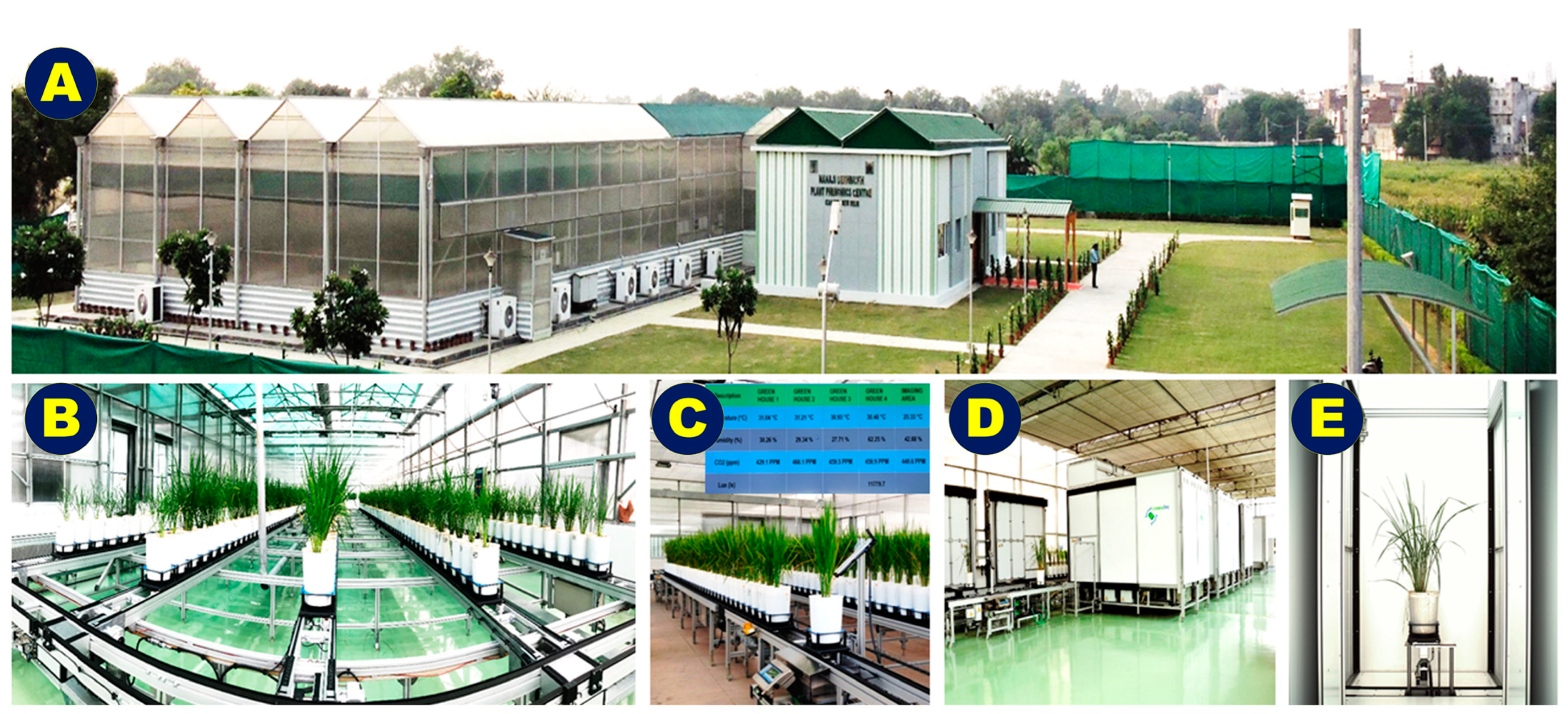
2.1. Experimental Set Up and Growth Condition

A pot culture experiment was conducted using 157 recombinant inbred lines (RILs) developed from bi-parental crossing between two rice genotypes (BVD 109 and IR 20). The study was conducted inside the climate-controlled greenhouses established at the Nanaji Deshmukh Plant Phenomics Center (NDPPC), ICAR—Indian Agricultural Research Institute, New Delhi, India, during the kharif (July to October) season 2019 (Figure 1). The 25-day-old seedlings of each RIL line were transplanted into six sets of plastic pots containing 15 kg of puddled soil. The available soil nitrogen content was estimated to be around 113 kg/ha. One set of three pots was supplied with the recommended dose of fertilizer (at the rate of 120–80–60 kg/ha N–P–K, respectively) and considered as the N-sufficient (control) treatment. Another set of three pots was supplied with the recommended dose of fertilizer without a nitrogen source (at the rate of 0–80–60 kg/ha N–P–K, respectively) and considered as the N stress treatment. Plants were allowed to grow in contrasting N stress levels from transplantation to destructive sampling until 35 days after transplanting (DAT, maximum tillering stage) for the aboveground biomass estimation in the form of fresh weight (FW) and dry weight (DW).

A total of 990 pots were placed onto an automatic conveyor system installed at four greenhouses, and plants were grown under natural light conditions at the controlled sinusoidal temperatures of 32 °C (daytime) and 28 °C (nighttime). Relative humidity was maintained between 70 to 80% using an additive humidifier. Plants were grown under well-watered conditions at saturation moisture conditions (25% v/v basis). The recommended weed, pest and disease control practices for plant cultivation were followed. Complete randomized block design with three biological replications was maintained throughout the experiment. Pots planted with parents were kept in each greenhouse for normalization, and the positions of the pots were changed twice daily to minimize the greenhouse positional effect.

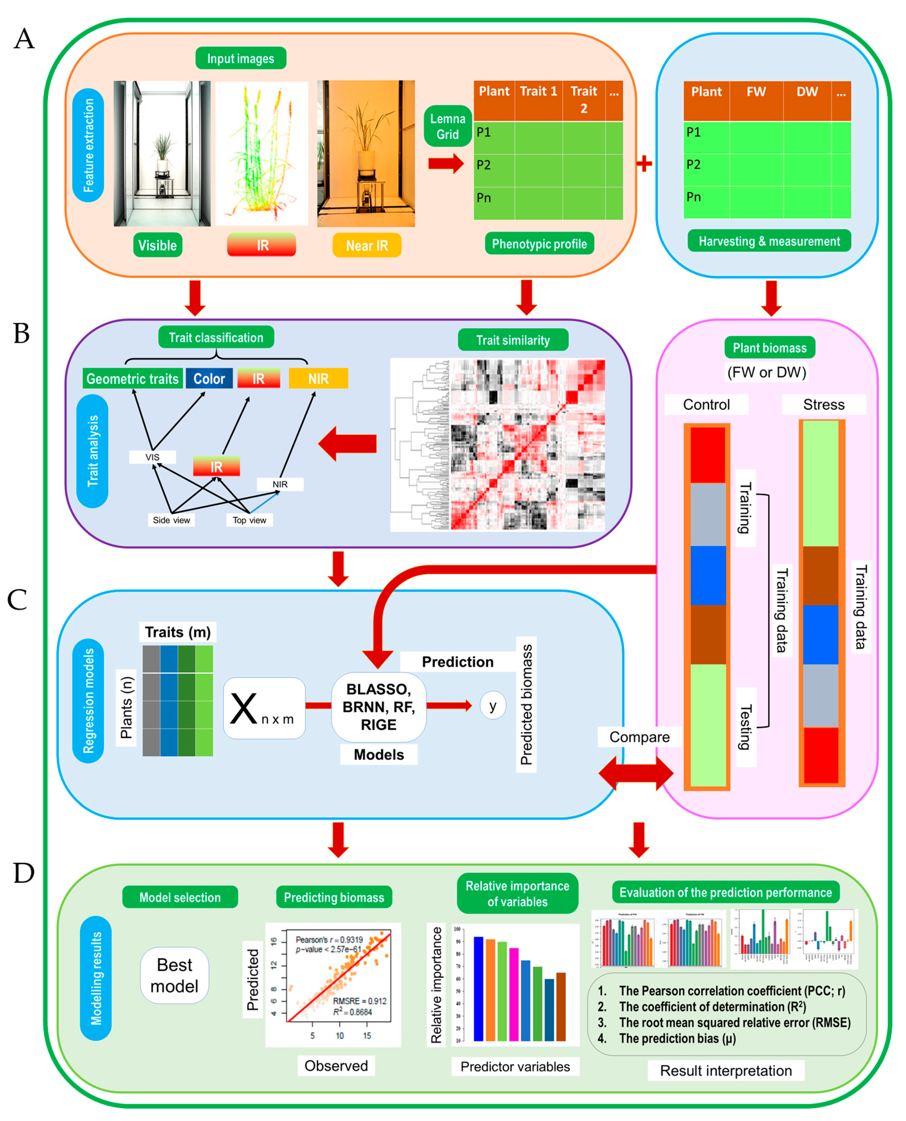
2.2. Image Data Acquisition, Processing and Analysis

RGB, IR and NIR images of all 990 RILs were acquired using a LemnaTec, Scanalyzer 3D imaging system (LemnaTec GmbH, Aachen, Germany) on the 65 days old plants just before destructively harvesting the plants for above-ground biomass estimation. Approximately 5000 RGB images were captured using an RGB camera (ProsilicaGT6400, spectral band: 400–700 nm, sensor: Allied Vision Technologies GmbH, Germany) and a constant fluorescent light source installed in the Scanalyzer 3D imaging system. In terms of size, 28-megapixel (6576 (X) ∗ 4384 (Y) resolution) color images were recorded from both the top and side views of the plants. During each time snap, five images were acquired per plant, viz., one from the top view of the plants at a 0° side-view rotational angle and four side-view images at rotations angles (0°, side view 1; 90°, side view 2; 120°, side view 3; 240°, side view 4). The raw image was acquired with a basic set up of an exposure of 32,000; a gain of 25; a gamma of 100; a red–white balance of 210; a blue–white–red balance of 135; and the double door closed option to avoid the shadowing effect of the side-view light source. Similarly, ~2000 NIR images were captured using gold eye P-032 SWIR Cool cameras. These have an in-built InGaAs sensor and a spectral band sensitivity of 900–1700 nm and were purchased from Allied Vision Technologies GmbH, Germany. A total of 2000 IR thermal images were acquired using a pearl eye P-030 LWIR camera with a spectral band sensitivity of 8000–14,000 nm and an inbuilt uncooled microbolometer sensor from Allied Vision Technologies GmbH, Germany, using the standard acquisition set up. Both NIR and IR images were acquired from two perspective views, one of each being captured at a 0° angle from a side view and a top view.

After the acquisition, ~450 gigabytes of images were transferred to an MP3 server (a Dell R910 server with 200 GB of RAM and two MD1200 storage devices with 24 TB). The stored images were processed using LemnaGrid software (LemnaTec GmbH, Germany). In brief, raw RGB images (12-bit BayerGR8 format) were demosaiced using an adaptive homogeneity-directed (AHD) algorithm to reconstruct a full-color image from the incomplete color output from an image sensor. The viewable pixels of these images were segregated into foreground and background pixels using HSI (hue, saturation and intensity) color space models along with an Otsu threshold value of 180. Additionally, free-form region of interest (ROI) filters were used in order to select the entire plant but cut out the visible parts of imaging hardware (e.g., lifter/turner). Logical operations such as AND/OR logics were used to combine the resultant images of diverse filters wherever required in the pipeline. Edge noise was removed through erosion and dilatation steps before bringing together all the parts identified as a plant into one object. Universal converters were used to convert processed images into object lists, binary images, or grey images wherever required in the image processing pipelines. Subsequently, the binary images of plants were analyzed for image features that consist of color classification of dark green- or brown-colored dry leaves. A hue-based HSI grey converter with two-level thresholds 44 to 180 was used to group the green and dry-leave pixels separately into two bins, and a histogram was made using pixel intensity in a range of values of 0–255.

2.3. Image Trait Feature Extraction

The size, area, height and geometrical dimensions of the object were calculated, and all five-angle images were used to estimate the projected shoot area (PSA) of the plant using the previously published methodologies [10,18,20] after making several modifications which can be described as follows. The calculated PSAs were compared with the actual plant size, which was determined using the destructively harvested plants. The conversion of the pixel area into millimeters (mm²) for the side-view images was achieved by multiplying pixel number by a constant of 0.308. The conversion of pixels from the top-view camera accounted for the changing distance effect as the plant grew closer to the camera. The height factor (centroid) was calculated based on the center of mass along the y axis from the side-view image and multiplied by a factor 1.8 (mm/pixel) to convert pixels into millimeters. The top view-specific constant was calculated by using Y = 0.00018/1.8 × X + 0.25, where, Y is the top view-specific constant, converting pixel area to millimeters, and x is the mean centroid for the two side-view images. The final calculation of the projected shoot area (PSA) was achieved by summing all the calibrated side-view and top-view images in mm². Further, the multiple sensor setups at NDPPC allowed us to calculate approximately 67 image-derived traits (referred to as i-traits hereafter). The description of each of the i-traits is mentioned in Supplementary Table S1. The general workflows of image acquisition, trait feature extraction and modeling to predict the plant biomass are depicted in Figure 2.

2.4. Machine Learning Modelling for Predicting Biomass

Once after imaging, all the plants were destructively harvested just above the soil surface to estimate the above-ground biomass (FW and DW). The biomass was estimated using the standard oven-drying method, in which the harvested samples were dried at 80 °C for five days until the sample weight reached a stable value and the actual biomass weight was measured using a precision scale. To understand the relationship between image-derived parameters and the biomass in rice, we employed multiple image-based features to predict FW and DW, as suggested by Chen et al. [19]. We used the open source web application (HTPmod) for modeling and data visualization at http://www.epiplant.hu-berlin.de/shiny/app/HTPmod/ (accessed on 15 November 2022). HTPmod is implemented into the shiny framework by integrating R’s computational power and professional visualization, including various ML approaches [32]. We used the PredMod application for the prediction of both fresh and dry weight using 16 different ML algorithms, as described in Figure 2. In this study, we selected 67 important i-traits; these can be used to investigate biomass prediction under control and N stress conditions in rice. Those i-traits were classified into four groups: geometric traits, color traits, IR and NIR traits (Supplementary Table S1). The physiological traits were mostly comprised of color-related traits, NIR-related traits, and IR-related traits. Further, several biomass-related traits (projected shoot area, volume from LemnaGrid, and estimated biovolume) were computed based on previous reports and used to estimate the model efficiency of multiple-trait modeling over existing single-trait algorithms.

2.5. Machine Learning Algorithms

HTPmod application possesses 16 machine learning models, namely, Bayesian regularized neural networks (BRNN), Bayesian least absolute shrinkage and selection operator (BLASSO), Gaussian processes with non-linear polynomial function kernel (GP-POLY), LASSO and elastic-net regularized generalized linear models (GLMNET), ridge regression (RIDGE), support vector regression-linear method (SVM-linear), multivariate adaptive regression splines (MARS), Bayesian generalized linear model (BGLM), least absolute shrinkage and selection operator (LASSO), multivariate linear regression (MLR), generalized linear models (GLM), random forest (RF), stochastic gradient boosting machine (GBM), k-nearest neighbors algorithm (KNN), support vector regression-radial method (SVM-radial) and Gaussian processes non-linear radial function kernel (GP-Radial) to predict the biomass (such as FW and DW) using image-derived trait features. The different packages, viz., arm (BGLM), monomvn (BLASSO), brnn (BRNN), gbm and plyr (GBM), glmnet (GLM), glmnet and matrix (GLMNET), lm (MLR), kernlab (GP-Poly and GP-Radial), elasticnet (LASSO), kknn (KNN), earth (MARS), random forest (RF), ridge (elasticnet), e1071 (SVM-linear) and kernlab (SVM-radial), were used to train the machine learning models in HTPmod. In these models, the normalized phenotypic profile matrices X n×m for a representative list of phenotypic traits were used as the predictors (explanatory variables) and the measured DW/FW were used for the response variable Y.

The HTPmod application uses the caret package in R software to tune the parameters of the above machine learning algorithms. The caret package comprised a set of functions to facilitate the process of creating prediction models. It contains tools for data splitting, preprocessing, feature selection, model tuning by re-sampling and variable importance estimation. The root mean squared error (RMSE), coefficient of determination (R²) and mean absolute error (MAE) were calculated during parameter tuning, and the minimum RMSE value was considered in order to select the optimal model. According to the optimal models determined in this study, the parameter mtry of the RF algorithm was set to 8. Models were trained using 10-time cross validation on the training data using trcontrol function with a repeated CV method. The eps-regression type was used with the linear kernel type; the cost = 100 for SVM models and the tuning ranged from 0.001, to 0.01, 0.1, 1, 10 and 100. The ridge regression model was performed using a glmnet package with tunegrid alpha = 0, lambda = 0.0001 and trcontrol at 10 times validation. LASSO regression was performed using the glmnet package with tunegrid alpha = 1, lambda = 0.0001 and trcontrol at 10 times validation. Elastic net regression was performed using glmnet package with tunegrid alpha = 0.5, length = 10, lambda = 0.0001 and trcontrol at 10 times validation. We built GBM with shrinkage 0.01, 2-fold cross validation and ntrees of 1000. Knn models were built using caret, pROC and mlbench package using k value = 1:70. Two parameters, viz., ntree and mtry, were tuned in an RF algorithm. The parameter mtry is related to the number of splits per node in each tree and ntree is the number of decision trees. The accuracy of the random forest model is mainly influenced by the value of mtry. Thus, we trained the model using default ntree value of 500. To assess the relative contribution of each phenotypic trait to predicting the biomass, the relative feature importance for MLR model was estimated using a heuristic method which decomposes the proportionate contribution of each predictor variable to R². We choose the “%IncMSE” (increase in mean squared error) to represent the criteria of relative importance measure. The number of subset (nsubsets) criteria (counting the number of model subsets that include the variable) was used to calculate the variable importance, which is implemented in the “evimp” function.

2.6. Evaluation of the Prediction Model

To assess the predictive performance of all 16 models, we randomly divided the data set into training and testing (90:10%) data sets. We used a 10-fold cross-validation strategy to check the prediction power of each regression model. The shiny app was used to frame a training model on a 90% data set and then applied to predict biomass for the 10% testing data set. Later, a comparative analysis was performed between the manually measured actual biomass and predicted biomass in the testing data. The predictive performance was evaluated based on the Pearson correlation coefficient (PCC; r at p < 0.001 significance) between the predicted values and the observed values; the square of Spearman correlation coefficient (ρ²); the coefficient of determination (R²), which is equal to the fraction of variance explained by the model; and the root mean squared error of cross-validation (RMSE) and predictive bias (μ) between the predicted and observed values.

$$R^2=1-\frac{S{S}_{res}}{S{S}_{tot}}=1-\frac{{{\displaystyle \sum }}_{i=1}^n{\left(y_i-\widehat{y_i}\right)}^2}{{{\displaystyle \sum }}_{i=1}^n{\left(y_i-\overline{y_{}}\right)}^2}$$

$$RMSE=\sqrt{\frac{1}{n}{\displaystyle \sum }_{i=1}^n{\left(\widehat{y_i}-y_i\right)}^2}$$

$$\mu =\frac{1}{n}\cdot {\displaystyle \sum }_{i=1}^n\frac{{\widehat{y}}_i-y_i}{y_i}$$

where, SSres and SStot are the sum of squares for residuals and the total sum of squares, respectively; $\widehat{y_i}$ is the predicted value and $y_i$ is the observed value of the $i$th plant; $\overline{y_{}}$ is the mean of the observed values; $n$ denotes the sample size of the data set.

2.7. Data Analysis

We used R studio (version 4.1.2) and implemented open source web application (HTPmod and PredMod) with the shiny framework for computation and visualization of the different ML models, scatter graphs of principal component analysis (PCA), trait similarity maps, and Pearson correlation coefficients (PCC). HTPmod and PredMod are open source web applications for modelling and data visualization which are available at world wide web address http://compbio.nju.edu.cn/app/HTPmod/ (accessed on 15 November 2022) [32].

3. Results

3.1. Image-Based Feature Extraction and Trait Selection

In the present study, the general workflow of image-based prediction of biomass is depicted in Figure 2. A total of 67 image-based traits were extracted, which were classified into four categories, viz., geometric-, color-, IR- and NIR-related traits (Figure 2A,B). We used the open source web application (HTPmod) for high-throughput multivariate modeling and biological data visualization (http://www.epiplant.hu-berlin.de/shiny/app/HTPmod/) as accessed on 15 November 2022 and the PredMod module for the prediction of biomass traits using 16 different machine learning models (Figure 2C).

The results of PCA for dimensionality reduction showed that the first two principal components could explain more than 50% of the phenotypic variance presents in control, N stress and control + N stress data (Supplementary Figure S1A–C). The total cumulative phenotypic variance, explained by the first two principal components, was found to undergo a moderate reduction from 60.27 to 57.47% for the plants grown in control than in the N stress condition (Supplementary Figure S1A,B). The reduction in the phenotypic variation of plants grown in the N stress condition was mainly attributed to the negative environmental effect of the N stress condition. The combined (control and N stress) data analysis showed that the total cumulative phenotypic variation captured by the first two principal components was significantly higher (61.83%) compared to the results of the analysis conducted separately (Figure 3A). Therefore, the combined control + N stress dataset was selected for further analysis as it could capture the maximum possible phenotypic variation of the experiment. Moreover, the first principal component of the combined data set was clearly able to distinguish the plants grown under sufficient levels of or deficits of soil nitrogen using 67 image-derived traits (Figure 3A). The box plot analysis of actual biomass is depicted in Figure 3B. The results showed that the plants grown in sufficient N levels (control) were found to possess higher biomasses than the N stress-affected plants. The fresh biomass (FW) of plants ranged from 5 to 82 g in plants grown under control conditions and from 3 to 21 g in N stress-affected plants. The estimated dry biomass (DW) ranged from 1 to 19 g in the control and from 1 to 10 g in the N stress conditions (Figure 3B). A large variation was also noticed for the 67 image-derived features which were measured using RGB, IR and NIR imaging sensors.

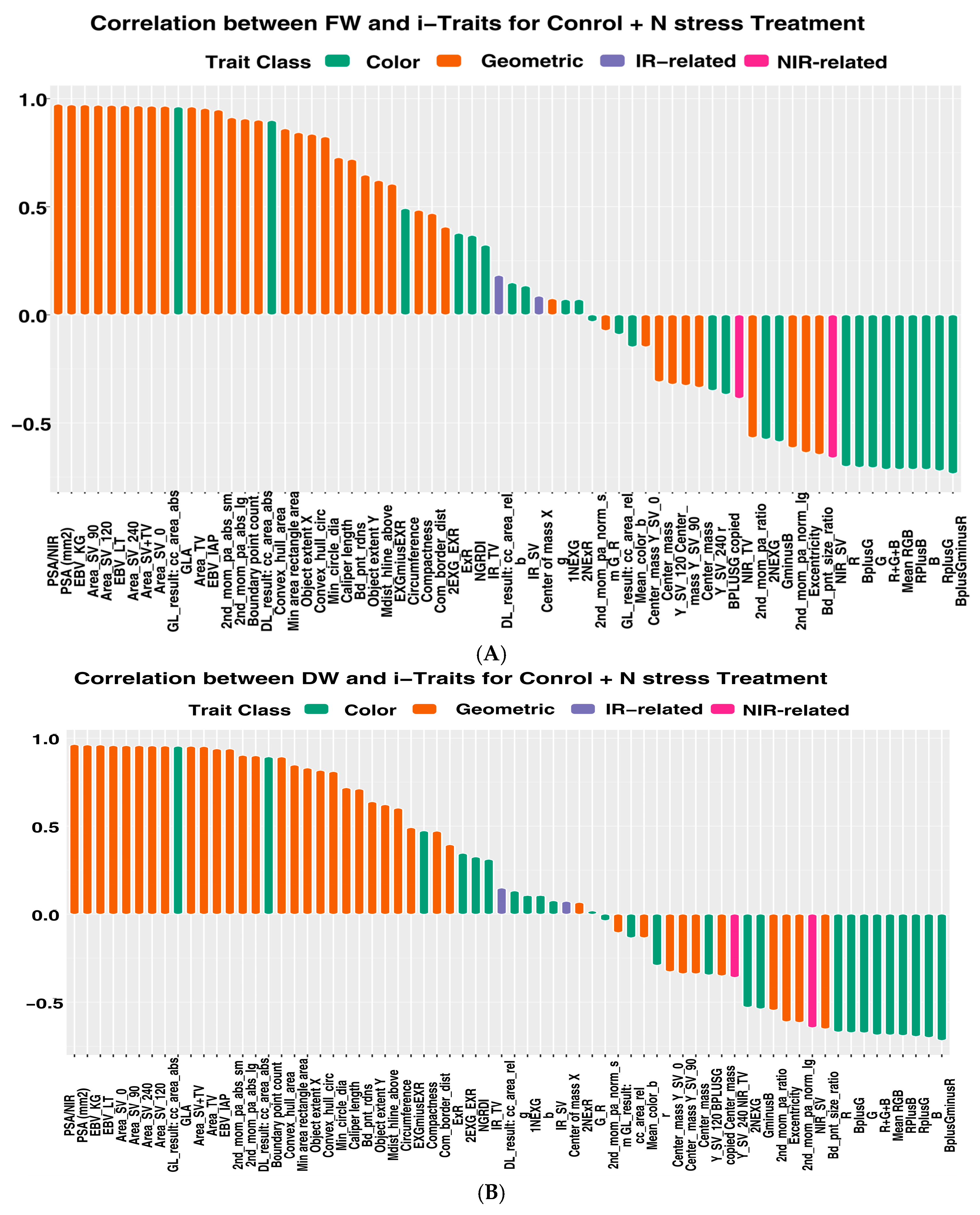
3.2. Trait Relationship among Each Other and Superior Trait for Biomass Prediction

The trait similarity analysis of image-derived traits was grouped into geometric-related traits, color-related traits, IR- and NIR-related traits. The heat map was drawn based on the Pearson correlation coefficient among the traits within the treatment groups (Supplementary Figure S2A,B). Similarly, the Pearson correlation coefficient was estimated in order to study the relationship between i-traits and response variables, i.e., FW and DW (Supplementary Figure S2A,B). The results of the similarity map showed that the traits within each trait group showed a very high positive correlation, indicating that these traits might be highly redundant descriptors of plant properties. The similarity map of i-traits derived from both control and N stress plants showed that geometric-related traits (PSA/NIR, PSA_hc, Area_SV_0, Area_SV_90, Area_SV_120, Area_SV_240 and Area TV) possessed very high positive correlations with each other (Supplementary Figure S2A,B) as well as with the response variables, i.e., FW and DW. Most of the architecture-related traits (except for the center of mass along with the Y axis, center of mass along with the X axis and normalized 2nd moments principal axis traits) were found to possess positive relationship between each other and biomass-related traits. This demonstrates the positive contribution of plant architecture traits to plant biomass accumulation. Similarly, most of the color-related physiological traits were positively correlated with each other and possessed negative relationships with biomass-related traits (Supplementary Figure S2A,B). The inverse relationship between plant nitrogen content and biomass, caused by the dilution effect, may be the reason for these negative associations. Among the color-related traits, GLA and DLA were found to have the strongest positive relationships with FW and DW. The IR-and NIR-related traits, acquired from two different perspectives, were observed to follow the same trend of possessing a very high positive correlation. However, NIR-related traits were found to have a very high negative correlation with biomass-related traits, a finding that was estimated from control plants. A lesser relationship or an absence of a relationship was found with plants grown in Nstress conditions. This may be due to the higher plant water status of plants grown in control conditions than in N stress conditions. These results suggested that high-throughput image-based features were mostly redundant and that the plant biomass accumulation was more dynamic than thought.

Further, we analyzed Pearson’s correlation coefficient (PCC) between the image-based traits (control + N stress) and the manually determined biomass traits (FW or DW). The results showed that more than 60% of i-traits had a very high positive correlation with manually estimated FW and DW biomass (Figure 4A,B). Among the trait groups, geometric-related traits, such as PSA/NIR, PSA_hc, Area_SV_0, Area_SV_120, Area_SV_240, Area_SV_90, PSA and Area TV, were found to possess a very high positive correlation irrespective of the FW or DW of the rice plants. Next to geometric-related traits, color-related traits, viz., GL and DL were found to possess very high positive correlation with FW and DW of the rice plants. A few color-related traits, such as EXG-, NGRDI- and IR-related traits (IR_SV and IR_TV), were identified to have moderate levels of positive relationships with FW and DW. Among the color-related traits, BplusG, G, RGB, R+G+B, B and RplusG were found to possess very high negative correlations with both FW and DW. These results suggested that those highly correlated image-based features may be considered as potential factors influencing plant biomass and able to be effectively utilized either alone or together for biomass prediction in rice.

3.3. Machine Learning Models for Prediction of Above-Ground Biomass

Thus, we first combined biomass measurements (fresh weight or dry weight) with single-image-based features, which were identified to possess very high predictive ability in terms of novelty and high positive correlation with biomass. The image-derived features used for predicting the biomass using simple linear regression models were Area_TV, Area_SV, PSA, PSA_hc, EBV_IAP, EBV_LemnaTec, EBV_keygene, GLA, relative ratios of PSA and NIR (PSA: NIR). To validate the prediction, a 10-fold cross-validation strategy was used to check the prediction power of each regression model. The Pearson correlation coefficients (r) between the predicted and actual values or the coefficient of determination (R²) and RMSE were used to evaluate the relationship between plant biomass accumulation and image-based features (

Table 1. Comparative evaluation of simple and multivariate machine learning model in predicting BIOMASS in rice.

Fresh Weight (Control+ N Stress)							Dry Weight (Control+ N Stress)
Simple Linear Regression Model	Models *	ρ2	R2	PCC	RMSE	µ	ρ2	R2	PCC	RMSE	µ
	SLRM_Area_TV	0.90	0.91	0.95	6.27	0.06	0.89	0.90	0.95	1.39	0.08
	SLRM_Area_SV	0.86	0.93	0.97	5.50	−0.48	0.83	0.94	0.97	1.10	−0.01
	SLRM_PSAhc	0.90	0.95	0.97	4.95	−0.20	0.87	0.95	0.97	1.04	0.03
	SLRM_EBVIAP	0.90	0.90	0.95	6.42	−0.38	0.88	0.90	0.95	1.33	−0.00
	SLRM_EBVLT	0.91	0.93	0.98	5.26	−0.17	0.89	0.93	0.97	1.11	0.04
	SLRM_EBVKG	0.91	0.94	0.97	4.95	−0.20	0.90	0.94	0.97	1.04	0.03
	SLRM_GLA	0.89	0.92	0.96	5.82	−0.44	0.89	0.93	0.97	1.15	−0.02
	SLRM_PSA:NIR	0.92	0.95	0.98	4.73	−0.04	0.90	0.95	0.97	1.01	0.06
Multivariate Machine Learning Model	BRNN	0.95	0.96	0.98	0.20	0.02	0.92	0.95	0.97	0.21	0.02
	BLASSO	0.94	0.96	0.98	0.22	0.01	0.92	0.95	0.97	0.23	0.01
	GP−Poly	0.95	0.96	0.98	0.23	0.02	0.92	0.95	0.97	0.24	0.02
	GLMNET	0.94	0.96	0.98	0.23	0.01	0.92	0.94	0.97	0.25	0.01
	RIDGE	0.94	0.96	0.98	0.29	0.01	0.92	0.94	0.97	0.25	0.02
	SVM−Linear	0.94	0.96	0.98	0.25	0.03	0.92	0.94	0.97	0.30	0.01
	MARS	0.94	0.96	0.98	0.21	0.03	0.90	0.94	0.97	0.33	0.00
	BGLM	0.94	0.96	0.98	0.33	0.00	0.92	0.94	0.97	0.31	0.02
	LASSO	0.94	0.95	0.98	0.36	0.01	0.68	0.94	0.97	0.32	0.01
	MLR	0.93	0.95	0.98	0.38	0.00	0.91	0.94	0.97	0.34	0.01
	GLM	0.93	0.95	0.98	0.38	0.01	0.91	0.93	0.96	0.23	0.04
	RF	0.94	0.94	0.97	0.22	0.03	0.91	0.92	0.96	0.34	0.07
	GBM	0.92	0.94	0.97	0.36	0.08	0.89	0.91	0.96	0.33	0.07
	KNN	0.88	0.93	0.96	0.38	0.10	0.86	0.90	0.95	0.60	0.10
	SVM−Radial	0.89	0.92	0.96	0.60	0.11	0.87	0.89	0.94	0.64	0.11
	GP−Radial	0.86	0.91	0.95	0.68	0.14	0.84	0.63	0.69	0.36	#

* The models prefixed as SLRM are simple linear regression models with response variables as either FW or DW, and the suffix names are i-traits features used as independent variables for linear regression models. The independent variables used for SLRM were AREA_TV: foreground pixels derived from top perspective view; AREA_SV: foreground pixels derived from side perspective view at 0° angle; PSAhc: projected shoot area calculated using top = view height constant and average side-view (0°and 90° angle) pixel count; EBV_IAP: estimated biovolume using formula used in IAP pipeline; EBV_LT: estimated biovolume using formula used in LemnaTec pipeline; EBV_KG: estimated biovolume using formula used in Key gene pipeline; GLA: green leave area pixel count using RGB image; PSA/NIR: relative ratio of projected shoot area with height constant; and grey intensity estimated using NIR sensor. Other models used were machine learning models that used all 62 image-derived features as independent variables and FW or DW as dependent response variables in a multivariable model. The multivariable machine learning models were, viz., Bayesian regularized neural network (BRNN), Bayesian least absolute shrinkage and selection operator (BLASSO), Gaussian processes-non-linear polynomial function kernel (GP-POLY) LASSO and elastic-net regularized generalized linear models (GLMNET), ridge regression (RIDGE), support vector regression-linear method (SVM-Linear), multivariate adaptive regression splines (MARS), Bayesian generalized linear model (BGLM), least absolute shrinkage and selection operator (LASSO), multivariate linear regression (MLR), generalized linear models (GLM), random forest (RF), gradient boosting machine (GBM), k-nearest neighbors algorithm (KNN), support vector regression-radial method (SVM-Radial) and Gaussian processes-non-linear radial function kernel (GP-Radial). The Pearson correlation coefficient (PCC at p < 0.001) between predicted and actual values or the coefficient of determination (R²; the percentage of biomass variance explained by the model) and RMSE were used to evaluate the relationship between plant biomass accumulation and image-based features and bias (µ). The positive value µ values were overestimated, or negative values were underestimated. # Denoted in the table is a negative infinitive error estimate.

). The performance indicators of simple linear regression models (SLRM) showed that the coefficient of determination (R²) for predicting DW ranged from 0.90 to 0.95 for Area_TV and PSA with height constant, respectively. A significant positive correlation (r = 0.95 to 0.97 @ p < 0.001 level) was found between all the selected i-traits and the DW of the rice plants. Among the image-derived traits estimated from different view angles, the area estimated from the side perspective view (R² = 0.94, r = 0.98 and RMSE = 1.10) outperformed the area estimated from the top perspective view (R² = 0.90, r = 0.95 and RMSE = 1.39) in rice. Further, in an attempt to understand the predictive ability of the independent variables derived from two different imaging sensors, the simple ratio between the PSA derived from the RGB sensor and the NIR grey intensity derived from the NIR sensor was estimated. Among the image-derived traits, the PSA/NIR trait (R² = 0.95, r = 0.97 and RMSE = 1.01) outperformed any other feature traits in the task of predicting FW or DW in rice. Therefore, PSA/NIR has the potential to be used as a single independent variable in predicting biomass in rice. The comparative evaluation suggested that, although the determination of co-efficient (R² = 0.95) and Pearson correlation coefficient (r = 0.97) which were estimated from PSA/NIR and PSA_hc traits were on par in terms of DW predictions, the prediction error (RMSE) was estimated to be lower in PSA/NIR (1.01) than in PSA_hc (1.04). In addition, the same trait was found to be the superior trait for FW prediction as well, with the highest R² (0.95) and PCC (0.98) values and with the lowest RMSE (4.73) and bias (−0.04) values.

3.4. Evaluation of Multivariate Models Using Performance Indicators

The predictive power of the multivariate model is considered superior to that of the univariate models as the latter utilizes only a single independent variable for predicting the response variable (biomass). The predictive power of the multivariate model for biomass prediction can be increased by combining multiple independent phenotypic traits because plant biomass is a resultant trait of not just structural architecture traits but also density features (physiological properties). Hence, in order to investigate the use of image-derived features in plant biomass prediction, deep phenotyping data containing both structural (e.g., geometric traits) and physiological traits (e.g., color and plant moisture content as reflected by NIR-related traits) were used together. In order to further improve the predictive ability of the model, we used16 different multivariate predictive models to assess the relationship between i-traits and plant FW and DW (Table 1). Among the 16 models, a very high positive correlation was observed between i-traits and plant FW (ranging 0.95 to 0.98) and DW (up to 0.97). It was observed that plant fresh weight (FW) and dry weight (DW) of control+ N stress plants could be accurately predicted from image-based parameters using multivariate regression models. The models were evaluated based on prediction accuracy, Pearson correlation coefficient, and prediction error (RMSE and bias) parameters calculated from the control, N stress and control + N stress treatment groups separately (Supplementary Table S3). The models which had most accurate prediction R² and the Pearson correlation coefficient (PCC) with the lowest RMSE and bias (µ) values were considered to be the best prediction models. Among the 16 multivariate models, BRNN, BLASSO and GP-Poly were found to have the highest coefficient of determination value ≥ 0.95 compared to other models across treatments. Moreover, BRNN and BLASSO models were identified as outperforming all other models in terms of prediction accuracy, Pearson correlation coefficient. They also had the lowest RMSE and bias values, even when using control and N stress data set separately or together (Table 1 and Supplementary Table S3) to predict FW and DW.

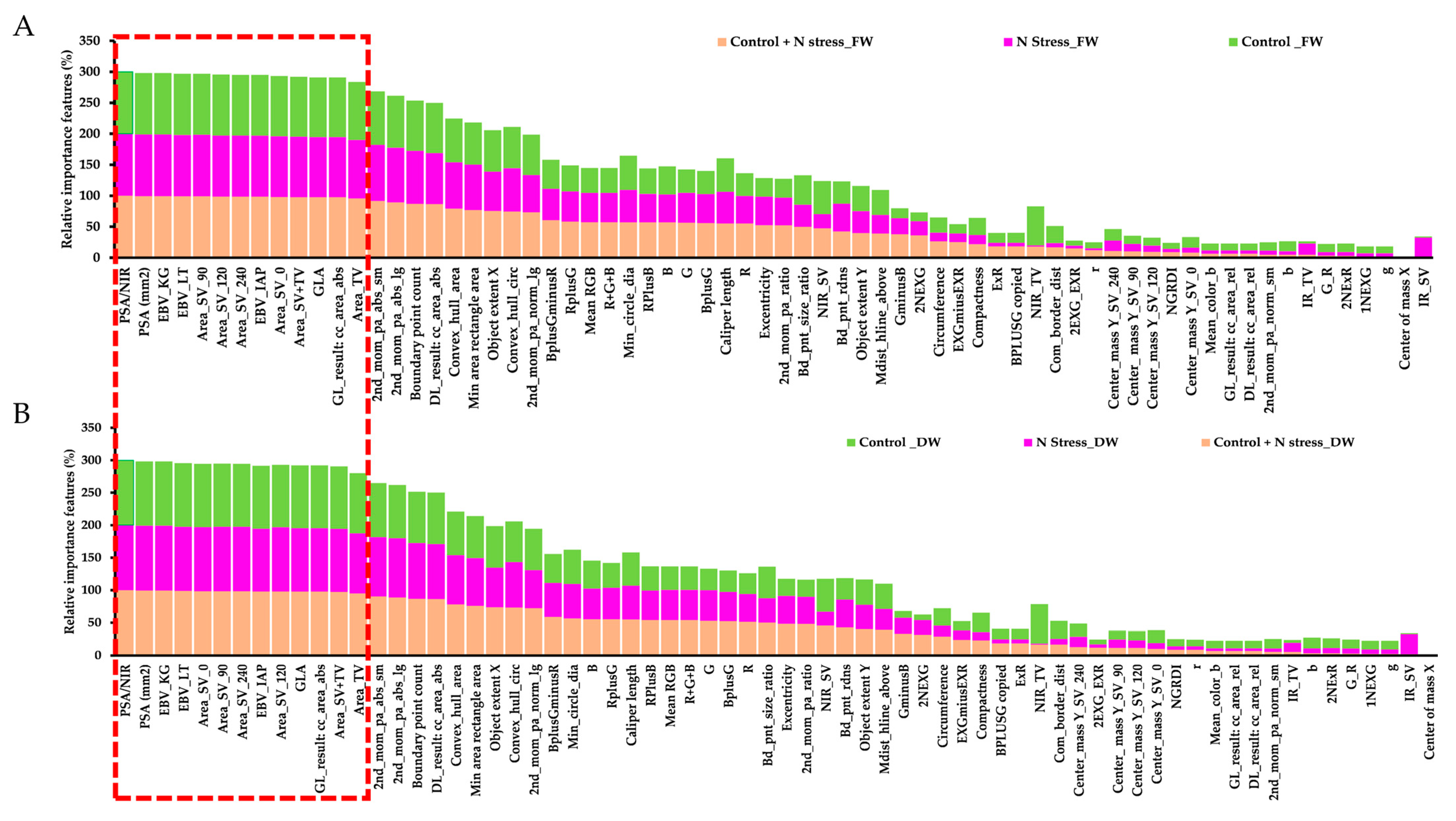
3.5. Relative Significance of Various Image-Based Features in Predicting Plant Biomass

The relative importance of image-based features was classified into four groups: (i) plant geometric- (biomass and plan architecture) and (ii) color-related features; (iii) IR signal- and NIR signal-based traits. The last three types of features reflect plant physiological properties and can be considered as plant biomass- and architecture-related traits and are thus related to plant fresh or dry weight. The geometric features showed the most predictive power among the four groups for the prediction of both FW and DW across plants from the control, N stress and control + N stress treatment groups (Supplementary Figure S9A,B). The relative ratio of PSA/NIR showed higher predictive capability for both FW (Supplementary Figure S9A) and DW (Supplementary Figure S9B). Not only did architectural traits such as 2nd_mom_pa_abs_sm, 2nd_mom_pa_abs_lgand boundary point count (R² > 0.816), Convex_hull_area (R² = 0.742), WidthSV (R² = 0.670), min area rectangle area (R² = 0.712), object extent X(R² = 0.692), and Convex_hull_circ (R² = 0.681) strongly contribute to fresh weight and dry prediction models, butphysiological traits such as DL_result: cc_area_abs (R² = 0.814), NIR.SV, Color.BplusGminusR (R² = 0.514), Color.RplusG (R² = 0.511) also strongly contributed to fresh weight and dry weight prediction models. This reveals new insights into the phenotypic determinants of plant biomass. Later, we studied the relative importance (RI) of each feature in predicting biomass using a full model across the treatment groups of plants (control, N stress and control + stressed plants). The RI of a feature in a BRNN model was calculated and the top ten most important features in the full model for predicting FW and DW were found to include both architectural and physiological traits. PSA/NIR, projected shoot area (PSA), Area_SV_0, Area_SV_90, Area_SV_120, Area_SV_240, and green leaves result cc_002.Color Class Area Absolut were the top-ranked features, each of which can considered as a representation of plant biomass of both FW (Figure 5A) and DW (Figure 5B). Additionally, the NIR-based features had greater predictive capability for DW (Supplementary Figure S9B) than for FW (Supplementary Figure S9A) in control + N stress plants, demonstrating the importance of NIR sensor data.

4. Discussion

High-Throughput Phenotypic Traits Precisely Estimate Biomass

The majority of conventional biomass estimation techniques rely on labor-intensive, time-consuming, and inconsistent field measurement and destructive sampling methods [3,4,5,6,7,8,9]. Whereas non-destructive imaging methods are not limited in this way, non-destructive imaging technologies give a faster, more precise method for plant phenotyping compared to the conventional destructive techniques used for measuring biomass. In recent years, plant biomass has been extensively studied using high-throughput phenotyping (HTP) approaches in several cereal crop species including rice, under controlled environmental [13,14] or field phenotyping facilities [20,21,22,23,24]. To date, two reports were found to estimate the biomass of rice seedlings up to the age of 6 weeks [16,17]. However, the presence of multiple models and algorithms for image-based prediction of biomass led us to work on assessing the comparative performance of different algorithms to identify best biomass prediction model for the specific task of estimating fully grown (70DAS) rice plants. Moreover, very little is known about the applicability of the wheat-, maize-, sorghum- and barley crop-specific models in rice plants [10,11,13,14,15,16,17,18,19]. The traits contributing to biomass, viz., size, number of leaves, tillering habits, phyllotaxy arrangement, and phyllochron pattern, are entirely different among the studied crop plants, at least compared to rice. Hence, the major objective of this study was to identify the novel image traits of plants grown under varied N stress levels and find the generic machine learning model fits for estimating the biomass of rice plants grown in contrast environmental conditions.

Initially, several studies were found to use foreground pixel count (area) as a single predictor variable to estimate the plant biomass in diverse crop plants, including rice [16]. Later, the image-based biomass was reported to be estimated using pixel counts from two orthogonal views of RGB images. Similar to these results, areas estimated from different orthogonal angles of side view were identified as relatively important traits in predicting biomass in our experiment (Figure 4A,B and Figure 5). Later, the sum of the foreground pixels was determined from visual images acquired from two orthogonal side views at 0° and 90° angles and top perspective views to use as the projected shoot area (PSA in kilo pixels). Then, PSA was used by several independent research groups as a single predictive variable for estimating biomass in rice [14,16]. Very high prediction accuracy (0.98) was reported for estimations of the biomass from single image-derived variable (PSA) and simple linear regression models in rice [16]. When we applied the same algorithms in our rice dataset, we could observe lower prediction accuracies of 0.90 to 0.94 (Table 1). The major reason for the higher prediction accuracy reported earlier may be related to the smaller number of sample size (N) and the lower genotypic variability (only two rice genotypes were used for phenotyping) utilized for the development of the model. Hence, this model was not considered as a generic algorithm suitable for measuring biomass in rice. Later, Klukas et al. [10] estimated digital bio-volume using a formula that uses both side-view and top-view pixel counts and reported them possess a positive relationship (0.85) with biomass in maize. In this case, the non-linear regression models were used to predict maize plants’ biomass and growth performance from image-derived PSA features. When we applied the EBV algorithm to our rice data set, we observed a lower prediction accuracy and higher prediction error. Among the three EBV-based algorithms, EBV_keygene out performed (R² = 0.94, r = 0.97, RMSE = 1.04) the models estimated from EBV_IAP and EBV_LemnaTec.

In another study, Neilson et al., 2015 [20] reported to develop an HTP workflow for predicting biomass in sorghum using PSA. This was the first attempt to estimate the PSA with a top-view height constant for normalizing the plant growth towards the imaging sensor and PSA_hc was expressed in mm². Similarly, Parent et al. [18] reported estimating the PSA along with the height constant for use in accurately predicting plant biomass in wheat. Hence, we applied this sorghum- and wheat-specific prediction algorithm in our rice experiment and observed the highest prediction accuracy (R² = 0.95, r = 0.97 and RMSE = 1.04) along with the highest positive trait relationship. This suggested that it is very much important to include the top view-specific height constants when handling a large population of diverse rice genotypes vis-a-vis estimating PSA from two contrasting treatment groups for biomass prediction. In addition, Campbell et al. [17], phenotyped around 373 diverse rice genotypes and estimated seven color-based traits along with PSA to predict biomass with high prediction accuracy (R² = 0.96) level. In the same trend, one color-related trait (GLA) was identified as possessing a very high relative importance among the color-related traits studied in our data set. GLA was also found to possess relatively higher prediction accuracy (R² = 0.93), with a very high positive trait relationship (r = 0.95) with the geometric trait (PSA, Area_SV_0 and Area_SV_90).

Among the trait groups, the relative importance of the NIR_TV feature was found to be highly variable for the prediction of FW or DW. The percentage of phenotypic variance captured by NIR_TV was recorded to be the highest for DW when using the model constructed with control + N stress data together rather than with control or N stress data separately (Figure 5). Hence, NIR_TV was considered for use along with geometric, color-related image traits in developing a highly generic biomass prediction model specific to diverse rice genotypes grown in contrasting stress environmental conditions. In general, the NIR_TV grey intensity is largely known for estimating plant hydration/moisture status. A fully hydrated plant sample absorbs most of the light spectrum incidence on the leaf, and meniscal light intensity is reflected back in NIR band long wavelength and vice-versa. In the same way, DW is known to possess a very high positive relationship with PSA. Therefore, a simple ratio between PSA estimated with height constant and NIR intensity from the top view image was used as a novel trait for improving the prediction accuracy of DW. In support of this fact, the basic understanding about deriving this (PSA/NIR) trait was related to the presence of an allometric relationship between FW and DW, which means that foliar water mass disproportionately increases with increased leaf dry weight [33]. The results showed that the performance of the PSA/NIR trait for the prediction of DW was almost on par with that obtained for the prediction performance of PSA with height constant alone (R² = 0.95 and r = 0.97). However, the inclusion of the NIR_TV feature along with PSA was found to improve the performance of the prediction model on par with any of the single or multivariate models used in our data set by reducing the prediction error to the lowest root mean square error (RMSE = 1.04 to 1.01).

Finally, we utilized around 67 image-derived traits acquired from three different imaging sensors (RGB, IR and NIR) and 16 multivariate machine learning models to accurately predict the FW and DW of rice plants. In this similar context, Chen et al., [19] used 36 image-derived traits from RGB, IR, NIR and fluorescence sensors and used 4 multivariate models to predict plant fresh and dry biomass weights in barley with a prediction accuracy of 0.96 using a random forest model. Similarly, Chen et al., extracted 54 image-derived features to predict plant fresh weight at 0.99 accuracy and dry weight at 0.89 in barley [11]. In our case, the best dry weight prediction model was identified to be BRNN, which had the highest prediction accuracy (R² = 0.95), Pearson correlation coefficient (r = 0.97) and prediction error (RMSE = 0.21). The reason for the better prediction performance of BRNN over the random forest algorithm may be due to the parametric assumption of most of the feature traits assigned in our data set. The estimated value for rice biomass (FW and DW) clearly followed a Gaussian distribution pattern in our population, and the image-derived traits were highly correlated with each other. In such Gaussian (or normal) distributed data sets, the BRNN is expected to perform better than a non-parametric random forest model that uses random and independent data sets. The reason for the reduced prediction accuracy of RF may be due to unknown explanations, as RF uses a black box algorithm for prediction. In contrast, Bayesian regularized neural networks are simple artificial neural networks used to develop generalized robust model in order to overcome the difficulty of over-fit or under-fit for the construction of a prediction model. Moreover, it minimizes a linear combination of squared errors and weights. It was found to be advantageous to apply the BRNN model in predicting the biomasses of diverse rice plants which were grown in contrasting N stress conditions. Moreover, variation in plant biomass can be attributed to the differential context of the feature traits, such as increases in the foreground pixel and decreases in the NIR signal. Because of this, the BRNN model can be used to predict a response variable using any data dispersion type, such as an exponential or a categorical class variable.

Recently, Hu et al. [1] used a combination of fractal dimension algorithms derived from the box-counting method along with traditional image-based features to improve the prediction model in rice. However, no studies have reported the image-based workflow for predicting fresh and dry biomass using HTP data comprising multiple novel features derived from different sensors and a large population of rice genotypes. Recently, our group reported the application of multiple imaging sensors (VIS and NIR) for predicting leaf fresh weight in rice [30]. In our study, green leaf proportion (GLP) from the VIS image and mean gray value/intensity (NIR_MGI) from the NIR image were used as inputs to develop an artificial neural network (ANN) model and we estimated the leaf fresh weight (LFW) in rice. Still, the prediction of biomass in rice possesses many inherent problems associated with estimating PSA or area from the side- and top-view images due to occlusion or the overlapping of rice leaves. In this case, more deep phenotyping research needs to be conducted for the accurate phenotyping of leaf length- (length of the leaf from base to tip) and leaf width-based predictions of PSA. In this direction, our group recently published a report on image-based prediction of leaf count using the deep learning model YoLo (you only look once) with a highest prediction accuracy of up to 98% [31]. Further, earlier reports also showed that the prediction of biomass uses per-pixel mass and machine learning regression models, which had been presumed to possess limited scope when the rice plants gain/loss weight, without any change in pixel area during the post-flowering period. Hence, it is imperative to develop a non-invasive imaging and data processing technique for precisely (R² = 1.00) estimating dynamic changes in biomass.

Machine learning models have been extensively used to predict plant biomass [11], classification/prediction plant health status (stress/non-stress) [12], gene expression and DNA methylation levels [25], etc. The detailed list of models, descriptions, and R packages used by different researchers for estimating biomass is given in Supplementary Table S2. When the BRNN model was compared to other regression models, it was observed that the BRNN model outperform other models in terms of (a) better predictive power, particularly when compared to the linear model, confirming the complex phenotypic architecture of biomass, and (b) practical biological interpretability and readily extractable information about the importance of each feature in prediction. The high prediction accuracy attained based on this model, particularly the across treatment (control + N stress plants) performance, suggested that solving the phenotyping bottleneck in biomass measurement in breeding applications might be feasible. Using image data and a reference dataset to train the BRNN model, it is possible to predict biomass in several large plant populations throughout the treatment of rice using high-throughput phenotyping technologies. However, it is a great challenge to find a predictive biomass model in terms of both treatment and environmental effects on biomass accumulation. The model’s application will necessitate testing experiments with similar conditions to those of the reference experiment.

This conclusion was supported firstly by the observation that the model has greater predictive power of plant biomass in rice with two treatments, control and N stress, than in plants with a single treatment control Figure 5A,B and Figure S9A,B). However, when the model was applied to the combined dataset from across treatments (control, N stress and control + N stress), the prediction accuracy was found to be very high (R² = 0.96 and r = 0.98, average values from ten times of ten-fold cross-validation). Moreover, the destructive method made multiple measurements of the same plant over time impossible. With the development of new technology, digital image analysis has been used more broadly in many fields and plant research [13,14]. It allows for faster and more accurate plant phenotyping and has been proposed as an alternative way to infer plant biomass [14]. As for previous studies [14,15,16,21], we extended our biomass analyses from previous studies in which biomass was evaluated using only a single image-derived parameter (such as projected area) or several geometric parameters by integrating more representative features that accommodate both structural and physiological-related properties into a more advanced model. Despite the fact that the model’s predictive power was roughly higher than that of single feature-based prediction, such as projected shoot area (PSA) (Figure 5B,D), the model revealed the relative contribution of individual features in biomass prediction [4]. The data on the significance of each feature provided new insights into the phenotypic determinants of plant biomass outcome. Notably, several top-ranked features, such as PSA and NIR intensity, were revealed to have genetic correlations with dry weight and FW biomass [19]. This suggests that the top-ranked features may represent major phenotypic components of biomass output and can be used to dissect the genetic components underlying biomass accumulation. However, the current ability of models to characterize plant physiological-related properties from image data (such as chlorophyll content and leaf tissue water content, senescence, etc.) is still limited.

In summary, the compact crop architecture of rice poses challenges in predicting biomass non-destructively by using RGB sensors. Thus, researchers have reported using PSA as a surrogate trait for predicting plant biomass in rice [16,17]. The major limitation of these methods was related to the inverse relationship shown between prediction accuracy and the age of the rice plants. The reason for reduction in accuracy is presumed to be associated with complex leaf architecture, phyllotaxy, i.e., closely arranged tillers of rice plants that influenced the image-derived PSA by way of an occlusion effect. As clearly mentioned by Hairmansis et al., projected shoot area may be a suitable surrogate trait for predicting rice shoot biomass up to six weeks of age and up to 24 g of shoot fresh weight [16]. This team could achieve the highest R² value of 0.93 until the plant age of one month. However, other research groups working on wheat, barley, Arabidopsis, and sorghum crops applied different image-derived constants and used multivariate machine learning approach to improve the prediction accuracy up to 0.98. Thus, our novel aim was to develop the prediction model for fully grown rice plants up to the age of 65–70 days old plants to decipher the nitrogen stress tolerance. The hypothesis was to identify novel i-traits and apply machine learning models to improve the accuracy as reported earlier. To date, no report has been found on rice which aims to develop the biomass prediction model specific to the flowering stage. In addition to the identification of new constant (PSA: NIR), we tried to apply the already reported plant constants (specific for barley, sorghum and wheat) in our rice experiment and compared 16 ML models. This is the first report in rice that developed HTP workflow to predict biomass objects of very high occlusion (40 to 50 tillers and up to 100 leaf) developed using more than 100 genotypes grown in two different N stress condition. The Bayesian regularized neural network model may be considered as a generic model which can be used to estimate the plant biomass up to 80 g (DW) with R² = 0.95 accuracy. To improve the accuracy, researchers used multiple features to predict biomass and higher number of samples by using multiple linear regression model. Use of four machine learning methods to predict biomass in barley was performed using multi-sensor traits to improve accuracy and give more logical reasoning for prediction [19]. Thus, we aimed to predict biomass in rice by using 16 machine learning methods to observe the model accuracies across methods and different treatments. We also combined multi-sensor-derived traits to obtain novel traits like PSA/NIR intensity, which incorporates more biological meaning for biomass prediction. We performed the biomass prediction across treatments for illnessess such as nitrogen-deficient and nitrogen-sufficient conditions which will be helpful in different types of experiments. We used 67 high quality traits from RGB and NIR sensors which contain all types plant characteristics.

5. Conclusions

Rice is the major cereal crop and is grown worldwide to provide food and nutritional security to the global population. The phenotyping of large sets of the population in an automatic platform using non-invasive sensors is the need of the hour owing to the large deficiencies in the utilization of phenotyping and genotyping data in analytical breeding and rice crop improvement. The advantage of collecting spatio-temporal image-based phenotypic data constitutes a cutting-edge technological advancement in the prediction of the genomics region, governing stable or dynamic interactive loci. In this regard, the non-destructive prediction of biomass in rice plants places an inevitable prime position and necessitates accurate phenotyping for improving rice plants’ resilience to climate change. In this experiment, a novel multimodal i-trait (relative ratio of PSA/NIR) was identified as the best trait for the accurate prediction of biomass (both FW and DW) in rice. The predictive performance of PSA/ NIR trait was evaluated against prior known image-derived features that possess very strong linear relationships with biomass. Among the 16 machine learning models, BRNN was found to be the best model. With a biomass prediction accuracy of 0.95 in rice plants up to the age of 70 DAS and 80 g of dry weight. This model was also validated to be a generic model and can be used for predicting the plant biomass from nitrogen stress and unstressed plants. The rice-specific multivariate machine learning model (BRNN) was found to exhibit a superior performance compared to the single independent variable (PSA/NIR) in terms of prediction accuracy and prediction error. The demonstrated methodology and algorithms can be effectively utilized for predicting biomass in rice or potentially applied to other crop species for the non-invasive phenotyping of crop plants.

References

1. Hu, Y.; Shen, J.; Qi, Y. Estimation of Rice Biomass at Different Growth Stages by Using Fractal Dimension in Image Processing. Appl. Sci. 2021, 11, 7151. [Google Scholar] [CrossRef]
2. Toda, Y.; Wakatsuki, H.; Aoike, T.; Kajiya-Kanegae, H.; Yamasaki, M.; Yoshioka, T.; Ebana, K.; Hayashi, T.; Nakagawa, H.; Hasegawa, T. Predicting Biomass of Rice with Intermediate Traits: Modeling Method Combining Crop Growth Models and Genomic Prediction Models. PLoS ONE 2020, 15, e0233951. [Google Scholar] [CrossRef] [PubMed]
3. Zhu, G.; Peng, S.; Huang, J.; Cui, K.; Nie, L.; Wang, F. Genetic Improvements in Rice Yield and Concomitant Increases in Radiation-and Nitrogen-Use Efficiency in Middle Reaches of Yangtze River. Sci. Rep. 2016, 6, 21049. [Google Scholar] [CrossRef] [Green Version]
4. Matsubara, K.; Yamamoto, E.; Kobayashi, N.; Ishii, T.; Tanaka, J.; Tsunematsu, H.; Yoshinaga, S.; Matsumura, O.; Yonemaru, J.; Mizobuchi, R. Improvement of Rice Biomass Yield through QTL-Based Selection. PLoS ONE 2016, 11, e0151830. [Google Scholar] [CrossRef] [PubMed] [Green Version]
5. Corales, M.; Nguyen, N.T.A.; Abiko, T.; Mochizuki, T. Mapping Quantitative Trait Loci for Water Uptake of Rice under Aerobic Conditions. Plant Prod. Sci. 2020, 23, 436–451. [Google Scholar] [CrossRef]
6. Rakotoson, T.; Dusserre, J.; Letourmy, P.; Frouin, J.; Ratsimiala, I.R.; Rakotoarisoa, N.V.; Vom Brocke, K.; Ramanantsoanirina, A.; Ahmadi, N.; Raboin, L.-M. Genome-Wide Association Study of Nitrogen Use Efficiency and Agronomic Traits in Upland Rice. Rice Sci. 2021, 28, 379–390. [Google Scholar] [CrossRef]
7. Li, J.; Xin, W.; Wang, W.; Zhao, S.; Xu, L.; Jiang, X.; Duan, Y.; Zheng, H.; Yang, L.; Liu, H. Mapping of Candidate Genes in Response to Low Nitrogen in Rice Seedlings. Rice 2022, 15, 51. [Google Scholar] [CrossRef]
8. Bhandari, A.; Sandhu, N.; Bartholome, J.; Cao-Hamadoun, T.-V.; Ahmadi, N.; Kumari, N.; Kumar, A. Genome-Wide Association Study for Yield and Yield Related Traits under Reproductive Stage Drought in a Diverse Indica-Aus Rice Panel. Rice 2020, 13, 53. [Google Scholar] [CrossRef] [PubMed]
9. Yuan, J.; Wang, X.; Zhao, Y.; Khan, N.U.; Zhao, Z.; Zhang, Y.; Wen, X.; Tang, F.; Wang, F.; Li, Z. Genetic Basis and Identification of Candidate Genes for Salt Tolerance in Rice by GWAS. Sci. Rep. 2020, 10, 9958. [Google Scholar] [CrossRef]
10. Klukas, C.; Chen, D.; Pape, J.-M. Integrated Analysis Platform: An Open-Source Information System for High-Throughput Plant Phenotyping. Plant Physiol. 2014, 165, 506–518. [Google Scholar] [CrossRef] [Green Version]
11. Chen, D.; Neumann, K.; Friedel, S.; Kilian, B.; Chen, M.; Altmann, T.; Klukas, C. Dissecting the Phenotypic Components of Crop Plant Growth and Drought Responses Based on High-Throughput Image Analysis. Plant Cell 2014, 26, 4636–4655. [Google Scholar] [CrossRef] [PubMed] [Green Version]
12. Rahaman, M.M.; Chen, D.; Gillani, Z.; Klukas, C.; Chen, M. Advanced Phenotyping and Phenotype Data Analysis for the Study of Plant Growth and Development. Front. Plant Sci. 2015, 6, 619. [Google Scholar] [CrossRef] [Green Version]
13. Fahlgren, N.; Feldman, M.; Gehan, M.A.; Wilson, M.S.; Shyu, C.; Bryant, D.W.; Hill, S.T.; McEntee, C.J.; Warnasooriya, S.N.; Kumar, I.; et al. A Versatile Phenotyping System and Analytics Platform Reveals Diverse Temporal Responses to Water Availability in Setaria. Mol. Plant 2015, 8, 1520–1535. [Google Scholar] [CrossRef] [PubMed] [Green Version]
14. Golzarian, M.R.; Frick, R.A.; Rajendran, K.; Berger, B.; Roy, S.; Tester, M.; Lun, D.S. Accurate Inference of Shoot Biomass from High-Throughput Images of Cereal Plants. Plant Methods 2011, 7, 2. [Google Scholar] [CrossRef] [Green Version]
15. Arvidsson, S.; Pérez-Rodríguez, P.; Mueller-Roeber, B. A Growth Phenotyping Pipeline for Arabidopsis Thaliana Integrating Image Analysis and Rosette Area Modeling for Robust Quantification of Genotype Effects. New Phytol. 2011, 191, 895–907. [Google Scholar] [CrossRef] [PubMed]
16. Hairmansis, A.; Berger, B.; Tester, M.; Roy, S.J. Image-Based Phenotyping for Non-Destructive Screening of Different Salinity Tolerance Traits in Rice. Rice 2014, 7, 16. [Google Scholar] [CrossRef] [Green Version]
17. Campbell, M.T.; Knecht, A.C.; Berger, B.; Brien, C.J.; Wang, D.; Walia, H. Integrating Image-Based Phenomics and Association Analysis to Dissect the Genetic Architecture of Temporal Salinity Responses in Rice. Plant Physiol. 2015, 168, 1476–1489. [Google Scholar] [CrossRef] [Green Version]
18. Parent, B.; Shahinnia, F.; Maphosa, L.; Berger, B.; Rabie, H.; Chalmers, K.; Kovalchuk, A.; Langridge, P.; Fleury, D. Combining Field Performance with Controlled Environment Plant Imaging to Identify the Genetic Control of Growth and Transpiration Underlying Yield Response to Water-Deficit Stress in Wheat. J. Exp. Bot. 2015, 66, 5481–5492. [Google Scholar] [CrossRef] [Green Version]
19. Chen, D.; Shi, R.; Pape, J.-M.; Neumann, K.; Arend, D.; Graner, A.; Chen, M.; Klukas, C. Predicting Plant Biomass Accumulation from Image-Derived Parameters. GigaScience 2018, 7, giy001. [Google Scholar] [CrossRef] [Green Version]
20. Neilson, E.H.; Edwards, A.M.; Blomstedt, C.K.; Berger, B.; Møller, B.L.; Gleadow, R.M. Utilization of a High-Throughput Shoot Imaging System to Examine the Dynamic Phenotypic Responses of a C4 Cereal Crop Plant to Nitrogen and Water Deficiency over Time. J. Exp. Bot. 2015, 66, 1817–1832. [Google Scholar] [CrossRef]
21. Feng, H.; Jiang, N.; Huang, C.; Fang, W.; Yang, W.; Chen, G.; Xiong, L.; Liu, Q. A Hyperspectral Imaging System for an Accurate Prediction of the Above-Ground Biomass of Individual Rice Plants. Rev. Sci. Instrum. 2013, 84, 95107. [Google Scholar] [CrossRef]
22. Muraya, M.M.; Chu, J.; Zhao, Y.; Junker, A.; Klukas, C.; Reif, J.C.; Altmann, T. Genetic Variation of Growth Dynamics in Maize (Zea mays L.) Revealed through Automated Non-Invasive Phenotyping. Plant J. 2017, 89, 366–380. [Google Scholar] [CrossRef] [Green Version]
23. Neumann, K.; Zhao, Y.; Chu, J.; Keilwagen, J.; Reif, J.C.; Kilian, B.; Graner, A. Genetic Architecture and Temporal Patterns of Biomass Accumulation in Spring Barley Revealed by Image Analysis. BMC Plant Biol. 2017, 17, 137. [Google Scholar] [CrossRef] [PubMed] [Green Version]
24. Yang, W.; Guo, Z.; Huang, C.; Duan, L.; Chen, G.; Jiang, N.; Fang, W.; Feng, H.; Xie, W.; Lian, X.; et al. Combining high-throughput phenotyping and genome-wide association studies to reveal natural genetic variation in rice. Nat. Commun. 2014, 5, 5087. [Google Scholar] [CrossRef] [Green Version]
25. Zhang, X.; Huang, C.; Wu, D.; Qiao, F.; Li, W.; Duan, L.; Wang, K.; Xiao, Y.; Chen, G.; Liu, Q.; et al. High-Throughput Phenotyping and QTL Mapping Reveals the Genetic Architecture of Maize Plant Growth. Plant Physiol. 2017, 173, 1554–1564. [Google Scholar] [CrossRef] [PubMed] [Green Version]
26. Busemeyer, L.; Ruckelshausen, A.; Möller, K.; Melchinger, A.E.; Alheit, K.V.; Maurer, H.P.; Hahn, V.; Weissmann, E.A.; Reif, J.C.; Würschum, T. Precision phenotyping of biomass accumulation in triticale reveals temporal genetic patterns of regulation. Sci. Rep. 2013, 3, 2442. [Google Scholar] [CrossRef] [PubMed] [Green Version]
27. Cao, Q.; Miao, Y.; Wang, H.; Huang, S.; Cheng, S.; Khosla, R.; Jiang, R. Non-Destructive Estimation of Rice Plant Nitrogen Status with Crop Circle Multispectral Active Canopy Sensor. Field Crops Res. 2013, 154, 133–144. [Google Scholar] [CrossRef]
28. Erdle, K.; Mistele, B.; Schmidhalter, U. Comparison of Active and Passive Spectral Sensors in Discriminating Biomass Parameters and Nitrogen Status in Wheat Cultivars. Field Crops Res. 2011, 124, 74–84. [Google Scholar] [CrossRef]
29. Fernandez, M.G.S.; Bao, Y.; Tang, L.; Schnable, P.S. High-Throughput Phenotyping for Biomass Crops. Plant Physiol. 2017, 10, 17-00707. [Google Scholar]
30. Misra, T.; Arora, A.; Marwaha, S.; Ray, M.; Raju, D.; Kumar, S.; Goel, S.; Sahoo, R.N.; Chinnusamy, V. Artificial neural network for estimating leaf fresh weight of rice plant through visual-nir imaging. Indian J. Agric. Sci. 2019, 89, 146–150. [Google Scholar] [CrossRef]
31. Vishal, M.K.; Saluja, R.; Aggrawal, D.; Banerjee, B.; Raju, D.; Kumar, S.; Chinnusamy, V.; Sahoo, R.N.; Adinarayana, J. Leaf Count Aided Novel Framework for Rice (Oryza sativa L.) Genotypes Discrimination in Phenomics: Leveraging Computer Vision and Deep Learning Applications. Plants 2022, 11, 2663. [Google Scholar] [CrossRef] [PubMed]
32. Chen, D.; Fu, L.-Y.; Hu, D.; Klukas, C.; Chen, M.; Kaufmann, K. The HTPmod Shiny Application Enables Modeling and Visualization of Large-Scale Biological Data. Commun. Biol. 2018, 1, 89. [Google Scholar] [CrossRef] [PubMed] [Green Version]
33. Huang, W.; Ratkowsky, D.A.; Hui, C.; Wang, P.; Su, J.; Shi, P. Leaf Fresh Weight versus Dry Weight: Which Is Better for Describing the Scaling Relationship between Leaf Biomass and Leaf Area for Broad-Leaved Plants? Forests 2019, 10, 256. [Google Scholar] [CrossRef] [Green Version]
34. Koehrsen, W. Introduction to Bayesian Linear Regression—Towards Data Science. Medium. 2018. Available online: https://towardsdatascience.com/introduction-to-bayesian-linear-regression-e66e60791ea7 (accessed on 3 February 2023).
35. Gelman, A.; Jakulin, A.; Pittau, M.G.; Su, Y.-S. A Weakly Informative Default Prior Distribution for Logistic and Other Regression Models. Ann. Appl. Stat. 2008, 2, 1360–1383. [Google Scholar] [CrossRef]
36. Vasquez, M.M.; Hu, C.; Roe, D.J.; Chen, Z.; Halonen, M.; Guerra, S. Least Absolute Shrinkage and Selection Operator Type Methods for the Identification of Serum Biomarkers of Overweight and Obesity: Simulation and Application. BMC Med. Res. Methodol. 2016, 16, 154. [Google Scholar] [CrossRef] [Green Version]
37. Park, T.; Casella, G. The Bayesian Lasso. J. Am. Stat. Assoc. 2008, 103, 681–686. [Google Scholar] [CrossRef]
38. Burden, F.; Winkler, D. Bayesian Regularization of Neural Networks. In Artificial Neural Networks. Methods in Molecular Biology; Humana Press: Totowa, NJ, USA, 2008; Volume 458. [Google Scholar] [CrossRef]
39. Bai, Z.; Fahey, G.; Golub, G. Some Large-Scale Matrix Computation Problems. J. Comput. Appl. Math. 1996, 74, 71–89. [Google Scholar] [CrossRef] [Green Version]
40. Schuster, M.; Paliwal, K.K. Bidirectional Recurrent Neural Networks. IEEE Trans. Signal Process. 1997, 45, 2673–2681. [Google Scholar] [CrossRef] [Green Version]
41. Gianola, D.; Okut, H.; Weigel, K.A.; Rosa, G.J.M. Predicting Complex Quantitative Traits with Bayesian Neural Networks: A Case Study with Jersey Cows and Wheat. BMC Genet. 2011, 12, 87. [Google Scholar] [CrossRef] [Green Version]
42. Elsinghorst, D.S. Machine Learning Basics—Gradient Boosting & XGBoost. Shirin’s PlaygRound. 2018. Available online: https://shirinsplayground.netlify.app/2018/11/ml_basics_gbm/ (accessed on 3 February 2023).
43. Friedman, J.H. Greedy Function Approximation: A Gradient Boosting Machine. Ann. Stat. 2001, 29, 1189–1232. [Google Scholar] [CrossRef]
44. Generalized Linear Model. Available online: https://arxiv.org/pdf/2102.05497.pdf (accessed on 3 February 2023).
45. Friedman, J.; Hastie, T.; Tibshirani, R. Regularization Paths for Generalized Linear Models via Coordinate Descent. J. Stat. Softw. 2010, 33, 1. [Google Scholar] [CrossRef] [PubMed] [Green Version]
46. Al-Tamimi, N.; Brien, C.; Oakey, H.; Berger, B.; Saade, S.; Ho, Y.S.; Schmöckel, S.M.; Tester, M.; Negrão, S. Salinity Tolerance Loci Revealed in Rice Using High-Throughput Non-Invasive Phenotyping. Nat. Commun. 2016, 7, 13342. [Google Scholar] [CrossRef] [Green Version]
47. Trevor, H.; Qian, J.; Tay, K. An Introduction to ‘glmnet’. Available online: https://glmnet.stanford.edu/articles/glmnet.html (accessed on 3 February 2023).
48. Tibshirani, R.; Bien, J.; Friedman, J.; Hastie, T.; Simon, N.; Taylor, J.; Tibshirani, R.J. Strong Rules for Discarding Predictors in Lasso-type Problems. J. R. Stat. Soc. Ser. B 2012, 74, 245–266. [Google Scholar] [CrossRef] [Green Version]
49. Bach, F.R.; Jordan, M.I. Predictive Low-Rank Decomposition for Kernel Methods. In Proceedings of the 22nd International Conference on Machine Learning, Bonn, Germany, 7–11 August 2005; pp. 33–40. [Google Scholar]
50. Wu, T.-F.; Lin, C.-J.; Weng, R. Probability Estimates for Multi-Class Classification by Pairwise Coupling. J. Mach. Learn. Res. 2003, 5, 975–1005. [Google Scholar]
51. Zhiting, H. Gaussian Process and Deep Kernel Learning. In Probabilistic Graphical Models; Carnegie Mellon University: Pittsburgh, PA, USA, 2017; pp. 1–8. [Google Scholar]
52. Lee, S.; Wang, C. Probabilistic Graphical Models. 2017. Available online: https://www.ism.ac.jp/events/2017/meeting0222_24.html (accessed on 3 February 2023).
53. IBM. What Is the K-Nearest Neighbors Algorithm? IBM: Armonk, NY, USA, 2023. [Google Scholar]
54. Hechenbichler, K.; Schliep, K. Weighted K-Nearest-Neighbor Techniques and Ordinal Classification. 2004. Available online: https://epub.ub.uni-muenchen.de/1769/1/paper_399.pdf (accessed on 3 February 2023).
55. Columbia University Least Absolute Shrinkage and Selection Operator (LASSO). Available online: https://www.publichealth.columbia.edu/research/population-health-methods/least-absolute-shrinkage-and-selection-operator-lasso (accessed on 3 February 2023).
56. Januaviani, T.M.A.; Bon, A.T. The LASSO (Least Absolute Shrinkage and Selection Operator) Method to Predict Indonesian Foreign Exchange Deposit Data. In Proceedings of the International Conference on Industrial Engineering and Operations Management, Bangkok, Thailand, 5–7 March 2019. [Google Scholar]
57. Dodig, D.; Božinović, S.; Nikolić, A.; Zorić, M.; Vančetović, J.; Ignjatović-Micić, D.; Delić, N.; Weigelt-Fischer, K.; Junker, A.; Altmann, T. Image-Derived Traits Related to Mid-Season Growth Performance of Maize under Nitrogen and Water Stress. Front. Plant Sci. 2019, 10, 814. [Google Scholar] [CrossRef] [PubMed] [Green Version]
58. Brownlee, J. Multivariate Adaptive Regression Splines (MARS) in Python—MachineLearningMastery.Com. 2021. Available online: https://machinelearningmastery.com/multivariate-adaptive-regression-splines-mars-in-python/ (accessed on 3 February 2023).
59. Friedman, J.H. Multivariate Adaptive Regression Splines. Ann. Stat. 1991, 19, 1–67. [Google Scholar] [CrossRef]
60. Liang, Z.; Pandey, P.; Stoerger, V.; Xu, Y.; Qiu, Y.; Ge, Y.; Schnable, J.C. Conventional and Hyperspectral Time-Series Imaging of Maize Lines Widely Used in Field Trials. Gigascience 2018, 7, gix117. [Google Scholar] [CrossRef] [Green Version]
61. Voxco. Multivariate Regression: Definition, Example and Steps; Voxco: Surry Hills, Australia, 2023. [Google Scholar]
62. RColorBrewer, S.; Liaw, M.A. Package ‘Randomforest’; University of California: Berkeley, CA, USA, 2018. [Google Scholar]
63. Liu, Y.; Wang, Y.; Zhang, J. New Machine Learning Algorithm: Random Forest BT. In BT—Information Computing and Applications; Springer: Berlin/Heidelberg, Germany, 2012; pp. 246–252. [Google Scholar]
64. Saunders, C.; Gammerman, A.; Vovk, V. Ridge Regression Learning Algorithm in Dual Variables. In Proceedings of the Proceedings of the Fifteenth International Conference on Machine Learning (ICML 1998), Madison, WI, USA, 24–27 July 1998. [Google Scholar]
65. Anish Singh, W. Radial Kernel Support Vector Classifier. Available online: https://datascienceplus.com/radial-kernel-support-vector-classifier/ (accessed on 3 February 2023).
66. Shi, Y.; Li, P.; Yuan, H.; Miao, J.; Niu, L. Fast Kernel Extreme Learning Machine for Ordinal Regression. Knowledge-Based Syst. 2019, 177, 44–54. [Google Scholar] [CrossRef]
67. Yusof, K.W.; Babangida, N.M.; Mustafa, M.R.; Isa, M.H. Linear Kernel Support Vector Machines for Modeling Pore-Water Pressure Responses. J. Eng. Sci. Technol. 2017, 12, 2202–2212. [Google Scholar]
68. Peizhuang, W. Pattern Recognition with Fuzzy Objective Function Algorithms (James C. Bezdek). Siam Rev. 1983, 25, 442. [Google Scholar] [CrossRef]
Figure 1. Experimental set up at Nanaji Deshmukh Plant Phenomics Center (NDPPC), ICAR—Indian Agricultural Research Institute, New Delhi, India. (A) High-throughput phenotyping (HTP) facility comprises four climate-controlled greenhouses, an imaging area and server room, and an admin block. (B) Pot culture experiment in the climate-controlled green-house; (C) automatic weighing and watering station; (D) imaging area with chambers installed with RGB, IR, and NIR cameras to acquire top- and side-view images. (E) RAW images were acquired from a side perspective view at 0° angle.
Agriculture 13 00852 g001
Figure 2. Workflow for predicting biomass of rice plants through image-derived feature traits and ML models. (A) Manual and image data collection: VIS, IR and NIR images were acquired using standard image unit configuration (IUC) set up, and LemnaGrid software (LemnaTec, Scanalyzer3D system) was used for image processing and feature extraction. After imaging, plants were harvested to measure fresh (FW) and dry weight (DW) weight. (B) The image-derived trait features were classified into four groups, viz., geometric-, color-, IR- and NIR-related traits; Principal component analysis was used, and trait similarity map was constructed, to identify the novel i-traits for image-based biomass prediction. (C) The selected i-traits (projected shoot area, Area-SV-0, Area-SV-90, Area-SV-120 and Area-TV) were used as independent variables to predict response variable, i.e., plant biomass (FW and DW). A total of 16ML models were constructed using the group wise (control, N stress and control+ N stress) training and testing data sets (90: 10%, respectively) along with 10-fold cross-validation as a quality control feature. (D) Best performing machine learning model was identified using performance indicators such as Pearson correlation coefficient (r) at a p < 0.001 significance level, coefficient of determination (R2), root mean squared error (RMSE) and prediction bias (µ).
Agriculture 13 00852 g002
Figure 3. Scatter plots showing the results of principal component analysis (PCA) and novel i-trait selection. (A) The percentage of total phenotypic variance explained by the top two principal components estimated from control+ N stress. The component scores are shown in points, treatments are shown as colors (orange color code for control and blue color code for Nstress treatment) and loading vectors are represented as projected lines. (B) Box plot showing the distribution of fresh and dry weight data points across the treatments.
Agriculture 13 00852 g003
Figure 4. Pearson correlation coefficient was estimated to study the relationship between image-derived traits and response variables FW (A), and DW, (B), control + N stress treatment are displayed in a cluster column chart.
Agriculture 13 00852 g004
Figure 5. Cluster column chart showing the relative importance of i-traits in predicting FW and DW using BRNN and BLASSO models. Relative importance of image-derived features in predicting FW (A) and DW (B). The features highlighted in the red dash box are PSA: NIR, PSA, EBV_KG, EBV_LT and GLA.
Agriculture 13 00852 g005