Wheat Import Demand in Mexico: Evidence of Quantile Cointegration

Abstract

The decline in the production of basic grains in Mexico has intensified since the 1990s, with wheat (Triticum) being no exception. This reduction was covered by the growth of Mexican imports. The objective of this research was to analyze the import demand function for wheat from 1994, the time of the initiation of the North American Free Trade Agreement (NAFTA). An autoregressive distributed lag (ARDL) model revealed the change in the conditional mean import demand using variations in its determinants, the Global Indicator of Economic Activity (IGAE for its Spanish acronym) and the real exchange rate, as proxy variables for income and relative prices, respectively. However, the conditional mean is insufficient in a context of increasing foreign purchases of wheat and outliers. Through a quantile extension of the ARDL model (with the acronym QARDL), we then found that the change in imports, and the relevance of the determinants, differed across import levels. In the short term, the upper quantiles of wheat imports responded mainly to their history and the exchange rate. Meanwhile, in the long term, the IGAE and the exchange rate influenced the lower quantiles of imports. We conclude that there was an asymmetric response in the conditional distribution of imports. In other words, this study provides evidence of short- and long-term location asymmetry in wheat imports under NAFTA. The research contributes to the econometric study of basic grain imports. For the first time, the QARDL model is used to understand the relationship between imports and their determinants, and the circumstances under which its use is recommended are indicated. Therefore, a new econometric method is used, avoiding the linearity of the ARDL model, and thus allowing a detailed and accurate estimation of the demand for imports. Consequently, the estimates and conclusions obtained will undoubtedly help economic agents to make more efficient decisions, from national and international investors to government agencies responsible for the promotion of Mexican agriculture.

1. Introduction

Neoclassical economic theory [1,2] and post-Keynesian theory [3], even with their differences, agree that the principal determinants of the import demand function are its relative prices (in the domestic currency) and income. Empirically, these determinants have been represented by the real exchange rate and gross domestic product (GDP), respectively [4,5,6,7,8,9]. In recent years, with the availability of higher-frequency series, the Global Indicator of Economic Activity (IGAE in Spanish) has replaced GDP [10]. Both use the same methodology [11] but differ in their frequencies. That is, the former is monthly, while GDP is quarterly.

The import demand function has been estimated for various periods and with various econometric methodologies for the Mexican economy. A brief description of research prior to the year 2000 can be found in the research by Moreno-Brid [6], which generally incorporated the methodology pioneered in cointegration by Engle and Granger [12,13], a two-stage methodology consisting of a long-term and a short-term regression. Therefore, there can be, at most, one cointegration vector (the long-run equilibrium relationship).

After the year 2000, research was published by Cermeño and Rivera Ponce [10], Loria Diaz [5], and Romero [9], who used the Johansen cointegration test [14]. This test allowed them to prove the existence of multiple cointegrating vectors. Subsequently, Pacheco-Lopez [7] estimated the demand for imports using the methodology proposed by Pesaran and Shin: an autoregressive distributed lag (ARDL) model.

All these empirical studies have been essential to understanding the short- and long-term dynamics of total Mexican imports. However, a double research gap remains: in the product analyzed and in the methodology employed.

First of all, the import of a particular product does not have to behave like total Mexican imports. For this reason, it is of interest to analyze specific imports, such as wheat (Triticum), an essential grain for the Mexican population.

Regarding the methodology, the starting point is an ARDL model, which allows the change in the conditional mean of the dependent variable (wheat imports) associated with the change in independent variables (price and income) to be captured. However, the lack of domestic substitutes for a basic grain could generate a high dependence on imports, with these becoming less responsive to independent variables. Hence, across the import distribution, imports would respond differently to their determinants.

In this sense, could the change in the conditional mean provided by the ARDL model be sufficient for analyzing the relationship of imports with their determinants? Accordingly, we hypothesized in this research that the effects and significance of the real exchange rate and economic activity on wheat import demand would be a function of the import location in different quantiles. In other words, the response of imports would be asymmetric, with a conditional distribution, under the North American Free Trade Agreement (NAFTA). This agreement was aimed at eliminating or reducing barriers to trade and investment between Canada, Mexico, and the United States for the period from 1994 to 2020 (NAFTA was replaced by a treaty between Mexico, the United States, and Canada (T-MEC), signed on 30 November 2018 and beginning on 1 July 2020 [15]). Based on the information available at the time of our estimation, this study covered the period from 1994 to 2018. To test our hypothesis, we started with the autoregressive distributed lag (ARDL) model, and it is contrasted with its quantile extension, the QARDL model.

This paper contributes to the empirical study of import demand. For the first time, the QARDL model is used to analyze wheat, combining cointegration with quantiles. In addition, by focusing on a specific and essential import for Mexicans, given that the imports of one grain do not have to behave like the total imports, aggregation bias is avoided. Consequently, the estimates and conclusions obtained will undoubtedly help economic agents to make more efficient decisions, from national and international investors to government agencies responsible for the promotion of Mexican agriculture.

This article is divided into seven sections, beginning with this introduction. The second section focuses on describing the main international trade theories, and thus explaining what causes the trade flow among countries. The third section describes wheat import behavior under NAFTA, emphasizing the causes and consequences. The materials and methods used are then described in the fourth section. Next, the results and a discussion are presented in the fifth and sixth sections, respectively. Conclusions bring this research to a close in the seventh and final section.

2. Theoretical Framework of International Trade

There are various causes of the growth of imports and their counterpart, exports. In this sense, since the work of Smith and Ricardo, several theories that attempt to explain what motivates trade have been formulated. Based on the classification proposed by Raquel Gonzalez [16], theories are grouped into three main categories: classical theories, theories of international trade, and new theoretical developments.

2.1. Classical Trade Theories

In the last years of the eighteenth century, Adam Smith pointed out that free trade would cause each country to specialize in the production of goods in which they have an absolute advantage or that they can produce more efficiently than other countries [17]. In this sense, countries would import the goods in which they have an absolute disadvantage. For his part, in the early nineteenth century, Ricardo [18] showed that even if a country has an absolute disadvantage with respect to another country, if the relative costs (the cost of one good in terms of another) are different, trade between countries is possible and beneficial. In other words, the less efficient country should specialize in the production and export of the good with a lower absolute disadvantage. Thus, we say that the country has a comparative advantage in this good. Consequently, the country would import the good in which the absolute disadvantage is greater, in other words, the good where it has a comparative disadvantage.

It is worth mentioning that Ricardo’s theory of comparative advantage does not indicate why relative costs differ between countries. Heckscher’s and Ohlin’s works in 1919 and 1935 provide an answer, finding that different factor endowments would be the main cause of the difference in relative costs [19,20]. Thus, Heckscher and Ohlin’s theorem postulates that the good in which the relatively abundant factor is intensively employed in the country will be the good that is exported. Thus, the good that intensively uses the relatively scarce factor will be imported.

2.2. Theories of International Trade

International trade as explained by the theory of comparative advantage only considers inter-industry trade. In other words, countries export and import only products that come from different industries. This rules out the case where a country has both a comparative advantage and a comparative disadvantage in one product at the same time. Consequently, the current intra-industry trade flows (export and import of products of the same industry) cannot be explained, and alternative theories emerge.

During the 1960s, Verdoon’s study on trade between the Benelux countries (Belgium, the Netherlands, and Luxembourg) [21], as well as Bela Balassa’s research on the creation of the European Economic Community [22], mark the beginning of theoretical and empirical studies on intra-industry trade. Among the determinants of intra-industrial trade are the following:

• Trade in products that are substitutable in their consumption but differentiated in their inputs;
• Product differentiation;
• Economies of scale, as well as innovation and technological differences.

The presence of differentiated products, as well as economies of scale, have generated two types of fundamental models: the reciprocal dumping model [23] and the monopolistic competition model [24].

In the former, companies set a different price between exported products and those sold on the domestic market. In the second model, there are two contrasting situations. It resembles a monopoly in that the individual firm produces a product which consumers consider different from the varieties produced by the competition, so the firm has some leeway to fix the price. However, although the varieties are not exactly the same, they are substitutable, so competition remains. In short, both monopolistic competition and dumping generate trade between countries.

2.3. New Theoretical Developments

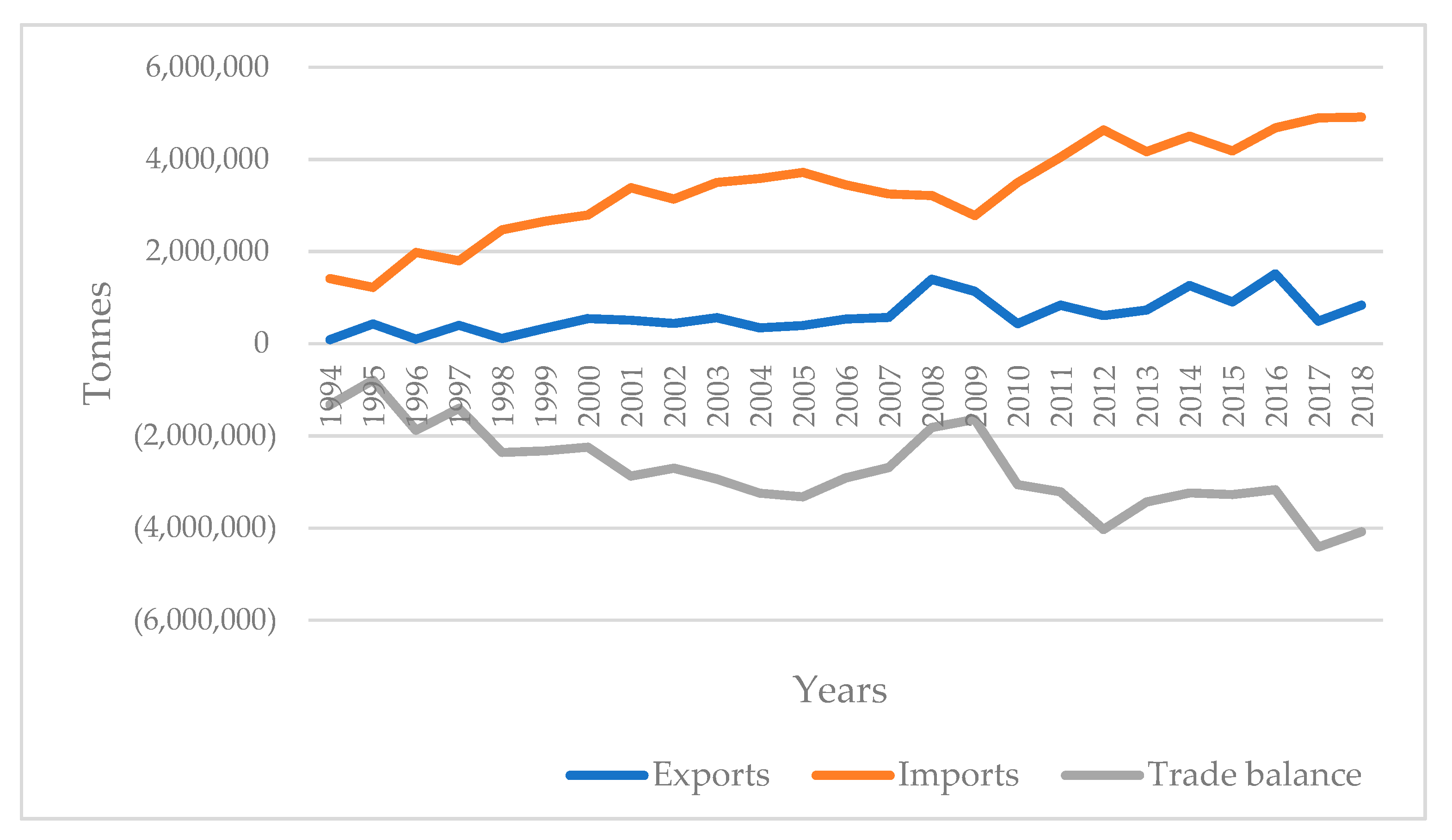
Previous theories had not given relevance to firms as a source of international trade. It was from the 1990s onwards that works showed that firms, even within the same industry, are different, which could influence the generation of trade [25,26,27]. For example, in a context of trade liberalization, low-productivity companies would be more likely to fail, while those with high productivity would survive and grow [28,29].

In other words, resources are shifted to high-productivity firms, whose growth increases the overall productivity of the entire industry, which will be higher in sectors with comparative advantages.

Likewise, the expansion of the production of exporting companies increases the demand for factors. This leads to an increase in factor prices, causing companies with low productivity to be unable to cover their costs and to have to exit the market. Therefore, the behavior of heterogeneous firms broadens the comparative advantages of countries, thus generating a source of profit by trade.

From the exposition of these three major categories in which the theories of trade have been grouped, it can be seen that they do not rule each other out, but rather complement each other, thus demonstrating that the causes of international trade are various and cannot be summed up in a single one. The following section shows what has happened in Mexico with respect to the wheat trade, specifically, importation of this grain since 1994, when NAFTA began.

3. Wheat in Mexico

NAFTA intensified agricultural specialization, meaning the export of fruits and vegetables increased, but not grains and oilseeds [30,31]. In this sense, there were winners and losers as a result of the specialization. Among the losers, wheat deserves special attention, as it is a key part of the Mexican population’s diet.

The Department of Agriculture, Livestock, Rural Development, Fisheries, and Food, as well as the National Institute of Statistics and Geography of Mexico (SAGARPA and INEGI in Spanish, respectively), have highlighted the importance of this crop. Wheat is the second most important cereal for Mexicans, only behind white corn, for which Mexico is self-sufficient. An average of 57.4 kg per capita is consumed each year [32]. INEGI, through the National Household Expenditure Survey, found that wheat accounts for 40% of the total cereal expenditure in Mexican households [33].

Despite the importance of wheat in the Mexican diet, domestic production has been reduced since the 1990s, and its demand has been covered with imports. For instance, in 1994, domestic production represented 74.59% of the total supply, while the rest came from overseas. By 2018, the Food and Agriculture Organization (FAO) indicated that this percentage had decreased to 37.43% [34] (see Figure 1).

The causes of the increase in imports can be divided into three historical stages [35,36]. From 1994 to 2007, there was a loss in the value of basic grains due to the increase in the United States’ subsidized supply, with the consequent discouragement of Mexican production. Subsequently, from 2008 to 2013, there was a period of an increase in value because international prices rose as a result of speculation and climate effects [37]. However, within the country, transnational corporations set lower prices than international prices, thus affecting the income of national producers. From 2014 onward, the decline in international oil prices marked a new stage in the loss of value of basic grains. All of this discouraged domestic production and led to an increase in imports.

With regard to consequences, the growth of foreign purchases of basic grains caused unemployment in the Mexican countryside due to the discouragement of Mexican production as a consequence of the loss of value mentioned above. At the same time, exports of fruits and vegetables had increased. However, these did not generate enough employment to absorb the unemployment caused by imports, thus increasing migration to the United States [37,38].

Another way of highlighting the significant growth of imports is through their impact on the trade balance. Undoubtedly, the aforementioned fall in domestic production had an impact on exports, which decreased, resulting in a significant deficit in the trade balance for this cereal [34] (see Figure 2).

4. Materials and Methods

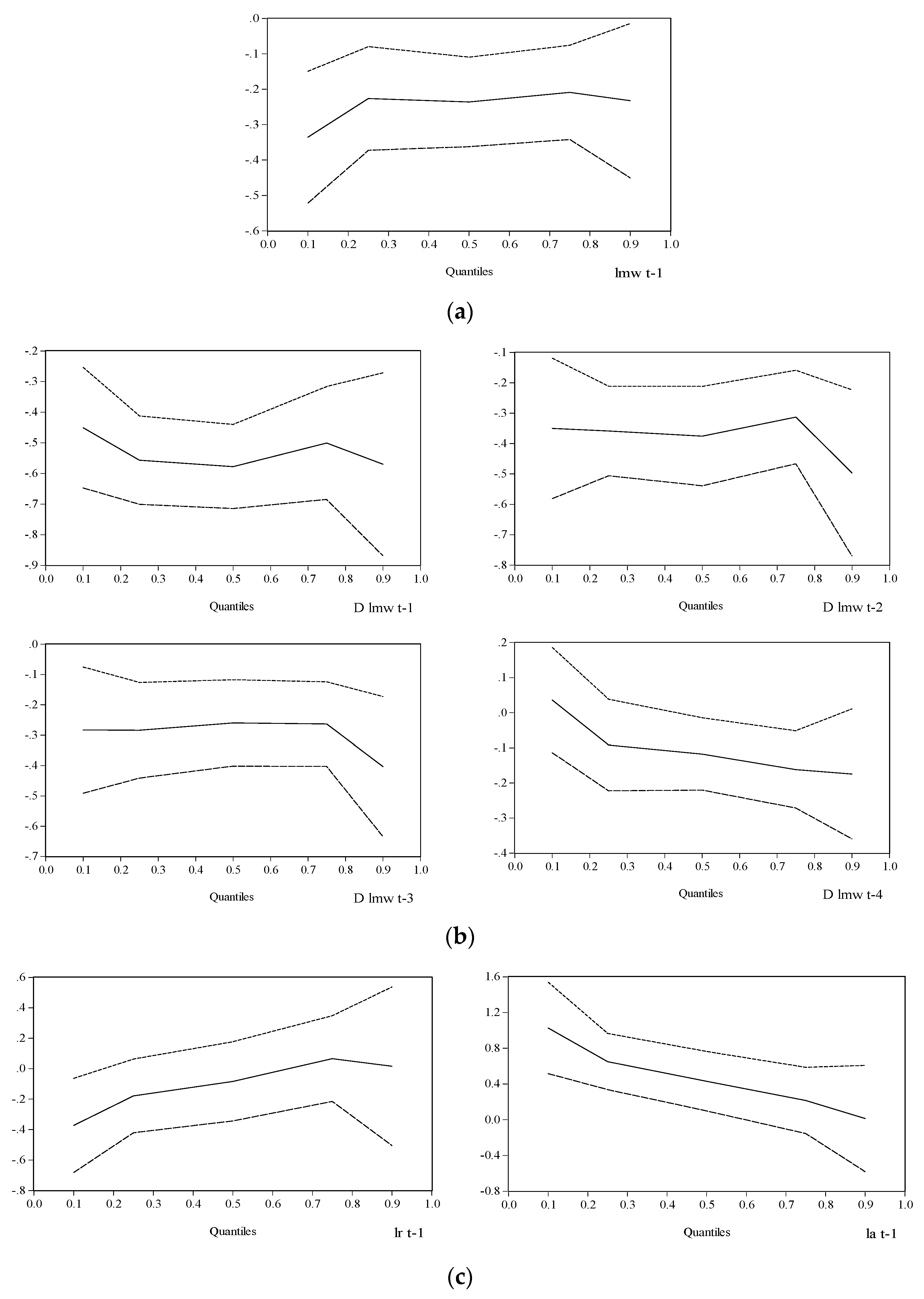
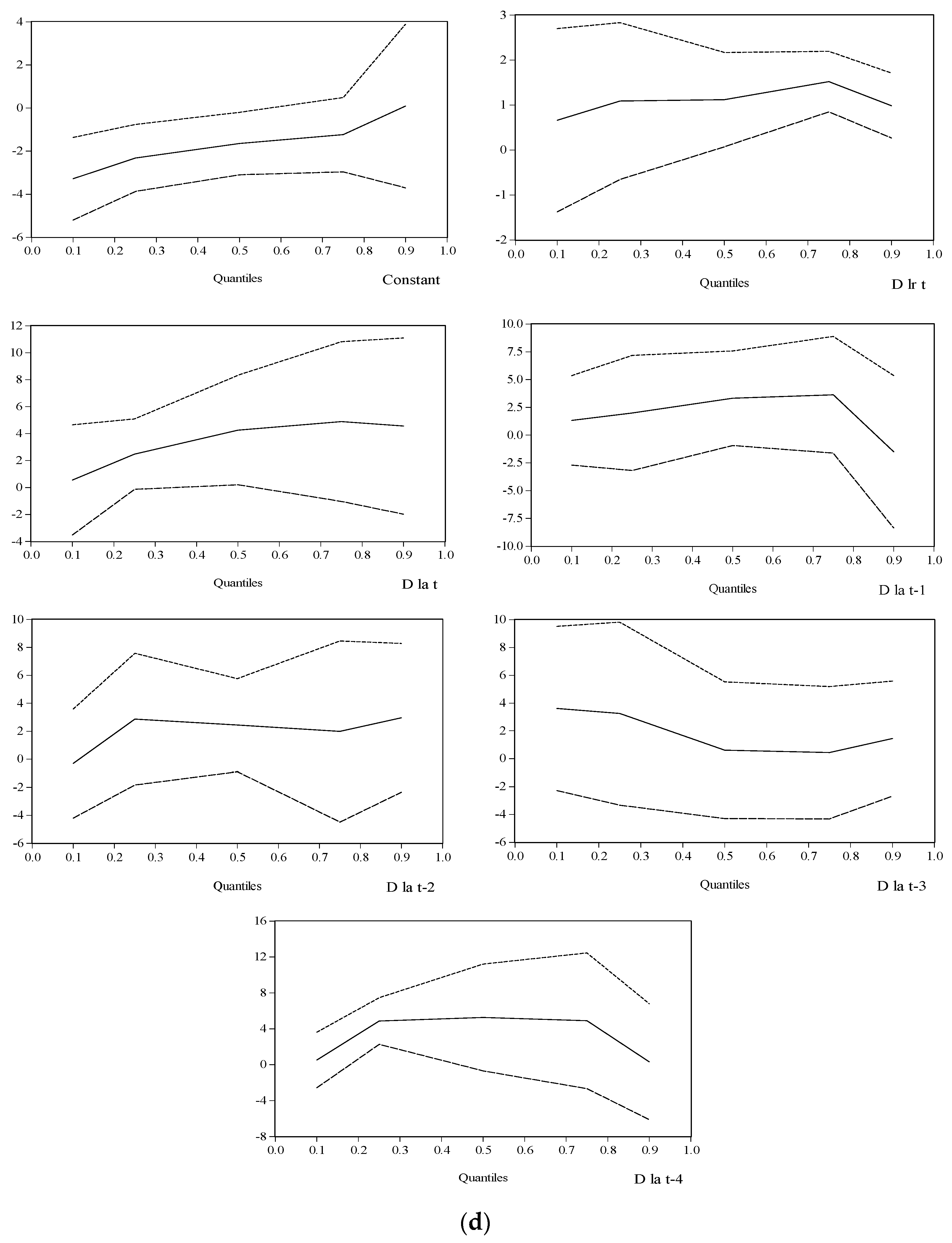
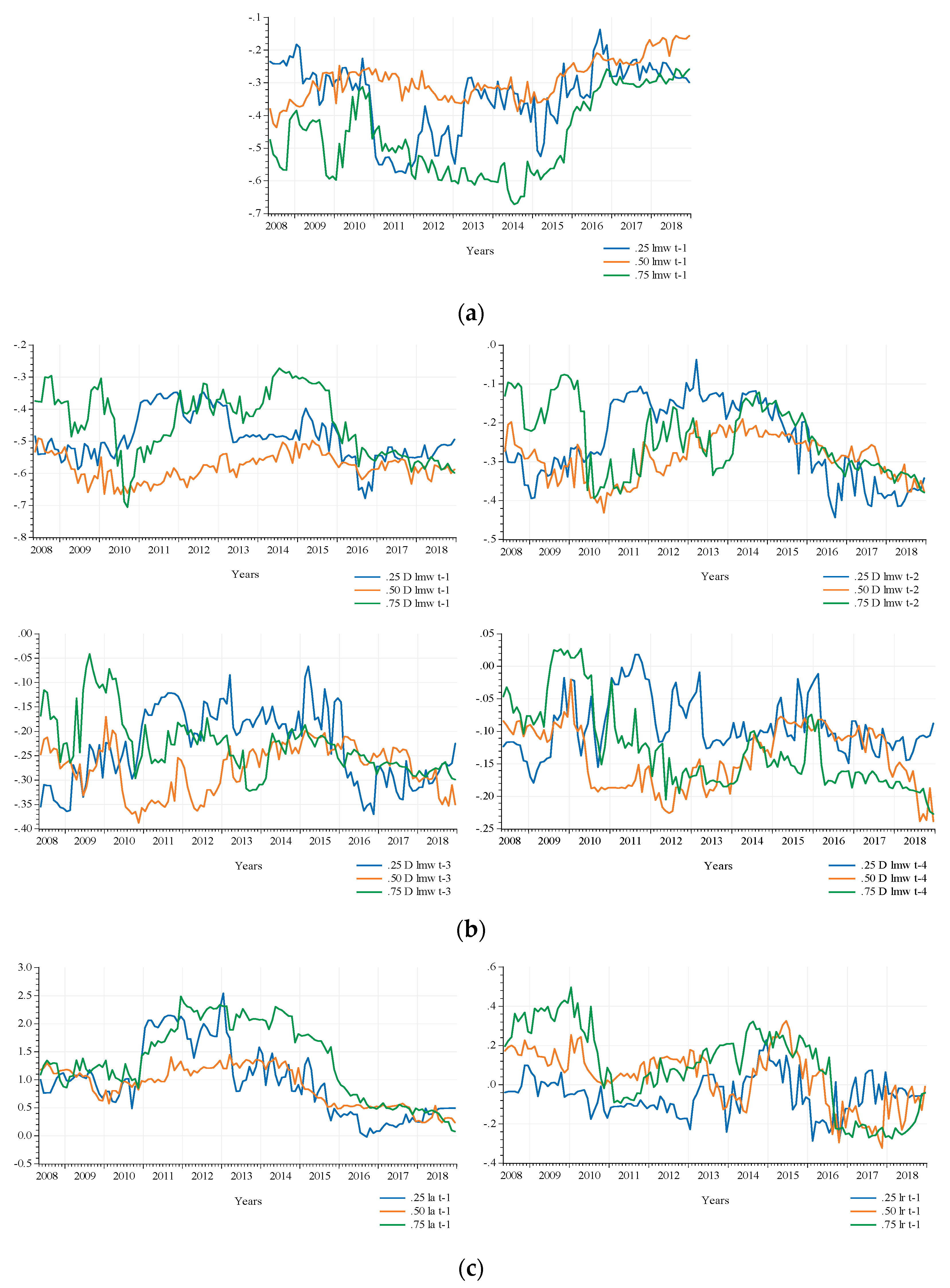
It has already been shown in the previous sections that there are several causes that motivate the growth of trade and, consequently, of imports. However, in order to have parsimonious modelling, and thus facilitate the interpretation of results, we rely on Neoclassical economic theory and post-Keynesian theory. Even with their differences, these theories agree that the principal determinants of the import demand function are its relative prices and income.

In this way, our methodology started with the following equation [4,5,6,7,8,9,10]:

$$l{m}_t={\beta }_{1}l{r}_t+{\beta }_{2}l{a}_t+u_t$$

(1)

where l represents the natural logarithm, m the imports, r the exchange rate, and a the Global Indicator of Economic Activity (IGAE) as proxy variables for relative prices and income. Coefficients ${\beta }_1$ and ${\beta }_2$ indicate the long-term process; this equation does not cover the short term. Therefore, we use an autoregressive model of distributed lag (ARDL) [39]:

$$l{m}_t={\sum }_{j=1}^{n1}{\gamma }_{j}l{m}_{t-j}+{\sum }_{j=0}^{n2}\pi l{r}_{t-j}+{\sum }_{j=0}^{n3}\phi l{a}_{t-j}+v_t$$

(2)

by expressing this equation in an error correction model (ECM), the short and long terms are incorporated in the following equation:

$$\Delta l{m}_t=\rho l{m}_{t-1}+{\sum }_{j=1}^{n1}{\gamma }_j\Delta l{m}_{t-j}+\theta l{r}_{t-1}+\lambda l{a}_{t-1}+{\sum }_{j=0}^{n2}\pi \Delta l{r}_{t-j}+{\sum }_{j=0}^{n3}\phi \Delta l{a}_{t-j}+e_t$$

(3)

where $\Delta$ indicates a difference, $\rho$ is the adjustment coefficient, ${\gamma }_j$ is the autoregressive coefficient, $\theta$ and $\lambda$ are the long-term coefficients, $\pi$ and $\phi$ are the short-term coefficients, and $e_t$ is the uncorrelated residual.

We employ an ARDL model because it has several benefits; for example, it can be calculated using ordinary least squares (OLS). Moreover, this kind of model covers all possible classifications of the regressors into purely I(0), purely I(1), or mutually cointegrated. Without omitting that, we have a one-stage methodology, that is, in a single equation we have the short- and long-term effects of the covariates in the dependent variable [39,40,41].

It is worth mentioning that the ARDL model obtains the change in the conditional mean of the dependent variable related to a change in the independent variables. However, this relationship may change, depending on the location of the dependent variable in its own conditional distribution. To find out if such a change exists, the quantile autoregressive distributed lag (QARDL) model is used [42].

The idea is to carry out the ARDL estimation by using the quantile regression proposed by Koenker and Bassett [43]. Quantile regression is more robust to outliers and non-normality than OLS regressions [44]. In other words, if the information under study presents very large or small values, the mean is not representative, and it would be better to describe the center of the data from the median (the 0.5 quantile). Quantile regression is a nonparametric technique, meaning no distributional assumptions (e.g., normality in the residuals) are required to optimally obtain the residuals.

Quantiles, represented by τ, indicate where an observation lies in an ordered series. As an example, the 0.25 quantile is the value that places 25% of the information below and 75% above. In this way, quantile regression models the entire conditional distribution of the explained variable given the covariates, and not just the mean, as OLS does in ARDL. As a result, it is possible, for example, to determine how the covariates affect the first or fourth quantiles of the distribution of the dependent variable [44].

Basically, the QARDL model is an extension of ARDL, but in a quantile context [42]. In this sense, we have the following equation:

$$Q_{lm}{}_t={\sum }_{j=1}^{n1}{\gamma }_j\left(\tau \right)l{m}_{t-j}+{\sum }_{j=0}^{n2}\pi \left(\tau \right)l{r}_{t-j}+{\sum }_{j=0}^{n3}\phi \left(\tau \right)l{a}_{t-j}+v_t\left(\tau \right)$$

(4)

where $\tau$ indicates the quantile $(0<\tau <1)$. By representing the above equation in an ECM, we arrive at the following expression:

$$Q_{\Delta lm}{}_t=\rho \left(\tau \right)l{m}_{t-1}+{\sum }_{j=1}^{n1}{\gamma }_j\left(\tau \right)\Delta l{m}_{t-j}+\theta \left(\tau \right)l{r}_{t-1}+\lambda \left(\tau \right)l{a}_{t-1}+{\sum }_{j=0}^{n2}\pi \left(\tau \right)\Delta l{r}_{t-j}+{\sum }_{j=0}^{n3}\phi \left(\tau \right)\Delta l{a}_{t-j}+e_t\left(\tau \right)$$

(5)

Recall that OLS estimator ($\widehat{\beta }$) produces the mean value that minimizes the sum of squared residuals. In contrast, the quantile regression estimator $({\widehat{b}}_{\tau })$ obtains the value that minimizes the sum of the absolute weighted residuals, in which the part with fewer observations receives a higher weighting [43,44], symbolically:

$${\widehat{b}}_{\tau }=\underset{bϵℝ}{\min }[{\sum }_{l{m}_t\ge b}\tau \left|e_t\right|+\sum _{l{m}_t<b}\left(1-\tau \right)\left|e_t\right|]$$

(6)

By obtaining ${\widehat{b}}_{\tau }$, we find the effect of the covariates on the quantile τ of the dependent variable.

In our analysis, national and monthly data for Mexico were utilized for 1994–2018. The Global Indicator of Economic Activity [11] and the real exchange rate index [45], represented by la and lr, were used to quantify their effects on the data distribution of Mexican wheat imports [46], described by lmw. Variables were seasonally adjusted (base 2013 = 100).

5. Results

A previous step to estimate the demand for imports was to determine the order of integration of the study variables.

Table 1. Unit root test.

Variable	Augmented Dickey–Fuller			Phillips–Perron
	CT	C	NCT	CT	C	NCT
lmw	−3.659 **	−2.367	−2.307 **	−10.551 *	−5.385 *	−3.843 *
∆lmw	−10.165 *	−10.163 *	−10.129 *	−37.675 *	−37.542 *	−37.391 *
∆∆lmw	−14.308 *	−14.329 *	−14.354 *	−79.581 *	−79.764 *	−79.922 *
la	−2.891	−0.621	2.696	−2.648	−0.748	3.382
∆la	−6.266 *	−6.277 *	−5.717 *	−17.087 *	−17.108 *	−16.556 *
∆∆la	−13.000 *	−13.024 *	−13.047 *	−45.835 *	−45.928 *	−46.018 *
lr	−2.495	−2.490	0.220	−2.395	−2.397	0.378
∆lr	−9.891 *	−9.908 *	−9.918 *	−13.975 *	−14.000 *	−14.016 *
∆∆lr	−15.253 *	−15.280 *	−15.306 *	−35.092 *	−35.154 *	−35.226 *

Note: CT, C, and NCT refer to a random walk with the constant and trend, only the constant, and no constant or trend, respectively. The letter l indicates a natural logarithm and Δ expresses a difference. The null hypothesis is a non-stationary series. Superscripts * and **, denote rejection of the null hypothesis at the 0.01% and 0.05% levels of significance, respectively.

contains Augmented Dickey–Fuller and Phillips–Perron unit root tests [47,48]. It can be seen that wheat imports were I(0), while the rest were I(1). Therefore, the use of the ARDL and QARDL models was feasible.

The starting point was the ARDL model. The Schwarz information criterion was used to define its number of lags. The model was divided into four sections (see

Table 2. Autoregressive distributed lag (ARDL) model of Mexican wheat import demand (1994–2018).

Section	Variable	ARDL Equation (3)
1. Adjustment	lmwt−1	−0.26
		[0.062] **
2. Autoregressive	Δlmwt−1	−0.50
		[0.074] **
	Δlmwt−2	−0.34
		[0.075] **
	Δlmwt−3	−0.25
		[0.070] **
	Δlmwt−4	−0.09
		[0.057]
3. Long term	lrt−1	−0.05
		[0.100]
	lat−1	0.53
		[0.172] **
4. Short term	Constant	−2.24
		[0.905] **
	Δlrt	1.18
		[0.434] **
	Δlat	3.42
		[1.711] **
	Δlat−1	2.81
		[1.764]
	Δlat−2	3.18
		[1.723] *
	Δlat−3	1.23
		[1.742]
	Δlat−4	4.24
		[1.746] **

Note: Standard errors consistent with heteroscedasticity and autocorrelation in square brackets. Superscripts * and ** indicate significance at 10% and 5%, respectively.

). The first section contained the adjustment coefficient, which was negative and less than 1, as required by the theory of an error correction model [13]. The second section contained the autoregressive coefficients, which indicated the impact of the history of wheat imports on their current change. The long-term effects were found in the third section; its coefficients were the price and income elasticities of wheat imports, and it was noteworthy that the price elasticity was not statistically significant. In this sense, changes in the exchange rate did not produce changes in wheat import demand. The last section contained the short-term process; in this case, in addition to economic activity and its history, the exchange rate affected imports. Considering all these sections, the last one presented the highest coefficients, revealing that the dynamics of wheat imports largely resulted from their covariates in the short term.

Table 3. Bounds test for cointegration, diagnostic, specification, and goodness-of-fit tests.

Tests			p-Value
FC	6.14
tC	−4.18
R2	0.42
Adjusted R2	0.39
	Heteroscedasticity
White uncrossed terms	18.82		(0.129)
	Serial Correlation
Breusch–Godfrey	10.26		(0.593)
	Functional Form
Ramsey’s RESET	0.26		(0.609)
	Normality
Jarque–Bera	10.67		(0.005)
Significance	Critical Value Bounds
	F-Statistic		t-Statistic
	I(0)	I(1)	I(0)	I(1)
10%	3.17	4.14	−2.57	−3.21
5%	3.79	4.85	−2.86	−3.53
1%	5.15	6.36	−3.43	−4.1

Null hypothesis: No cointegration.

contains the results of various tests we applied to the ARDL model. The F_C and t_C statistics indicate cointegration variables. There are no problems of heteroscedasticity or serial autocorrelation. Moreover, the Ramsay Regression Equation Specification Error Test (RESET test) indicates an absence of specification problems (omission of relevant variables, incorrect functional form, and/or correlation between independent variables with the error term). Yet, even with these positive results, the ARDL model presents problems, such as minimum goodness of fit (R² and adjusted R²), as well as the absence of normality in the residuals.

These problems are due to the presence of outliers in wheat imports (see Figure 3). This figure was made with information from the Mexico central bank (BANXICO) and INEGI [45,46]. The beginning of 1995 stands out because of the devaluation of the exchange rate at the end of 1994. Subsequently, the year 1998 is a highlight, influenced by the El Niño phenomenon in the agricultural areas of Mexico between 1997 and 1998 [49]. In addition, 2006 stands out due to the rise in world food prices during the period of 2005–2008, with the price of wheat being no exception [50]. Another outstanding year is 2008, as a consequence of the instability of the exchange rate generated by the global financial crisis in the same year, starting with appreciation and followed by a process of depreciation from the eighth month onward [45]. Finally, we have 2012, the year following a severe drought in the northern and central states of the country, affecting about 60% of the nation’s land [51].

The absence of normality in the residual, as well as the minimal goodness-of-fit, gave us reason to re-estimate the ARLD, but now using quantiles. A quantile regression is more robust to non-normality since it is a non-parametric technique. Therefore, distributional assumptions are not required to optimally estimate the parameters [44].

In addition, the way the dependent variable (lmw_t) is distributed further justifies the use of a quantile autoregressive distributed lag (QARDL) model. For instance, Figure 4 contains the histogram of the lmw_t variable, in which a leptokurtic shape with negative skewness can be seen. The p-value of the Jarque–Bera statistic confirms a non-normal distribution. In this regard, the mean is not representative of the total wheat imports, and a quantile analysis through the QARDL model is preferred to model the leptokurtic and skewed distribution of the dependent variable [52,53].

The number of lags in the QARDL model corresponds to the number previously fixed in the ARDL modeling. Undoubtedly, the selection should be a function of each quantile. However, doing so would have involved an overly extensive methodology, which was beyond the scope of the present research. Plus, if the lags were a function of the quantile, this would not only have increased the complexity but would also have made it impossible to compare the results between quantiles, or with the ARDL model.

Table 4. Quantile autoregressive distributed lag (QARDL) model of wheat import demand (1994–2018).

Section	Variable	QARDL Equation (5)
		τ = 0.10	τ = 0.25	τ = 0.5	τ = 0.75	τ = 0.90
1. Adjustment	lmwt−1	−0.34	−0.23	−0.24	−0.21	−0.23
		[0.113] **	[0.088] **	[0.076] **	[0.080] **	[0.132] *
2. Autoregressive	Δlmwt−1	−0.45	−0.56	−0.58	−0.50	−0.57
		[0.119] **	[0.087] **	[0.083] **	[0.111] **	[0.181] **
	Δlmwt−2	−0.35	−0.36	−0.38	−0.31	−0.50
		[0.140] **	[0.089] **	[0.099] **	[0.093] **	[0.166] **
	Δlmwt−3	−0.28	−0.28	−0.26	−0.26	−0.40
		[0.126] **	[0.095] **	[0.086] **	[0.084] **	[0.140] **
	Δlmwt−4	0.04	−0.09	−0.12	−0.16	−0.17
		[0.091]	[0.079]	[0.062] *	[0.066] **	[0.112]
3. Long term	lrt−1	−0.37	−0.18	−0.08	0.07	0.02
		[0.188] **	[0.147]	[0.158]	[0.171]	[0.316]
	lat−1	1.03	0.65	0.43	0.22	0.01
		[0.311] **	[0.190] **	[0.202] **	[0.225]	[0.361]
4. Short term	Constant	−3.28	−2.32	−1.65	−1.24	0.09
		[1.164] **	[0.944] **	[0.880] *	[1.049]	[2.307]
	Δlrt	0.66	1.09	1.12	1.52	0.99
		[1.239]	[1.059]	[0.637] *	[0.409] **	[0.438] **
	Δlat	0.56	2.48	4.26	4.89	4.56
		[2.484]	[1.587]	[2.471] *	[3.602]	[3.973]
	Δlat−1	1.33	1.99	3.32	3.63	−1.49
		[2.445]	[3.147]	[2.587]	[3.188]	[4.159]
	Δlat−2	−0.31	2.87	2.44	1.98	2.96
		[2.366]	[2.860]	[2.021]	[3.933]	[3.231]
	Δlat−3	3.62	3.25	0.61	0.43	1.45
		[3.587]	[3.998]	[2.983]	[2.890]	[2.512]
	Δlat−4	0.52	4.87	5.26	4.89	0.33
		[1.877]	[1.578] **	[3.613]	[4.593]	[3.925]

Note: τ indicates quantile, while superscripts * and ** represent significance at the 10% and 5% levels, respectively. Numbers in square brackets are standard errors consistent with heteroscedasticity and autocorrelation.

contains the QARDL estimation for the 0.10, 0.25, 0.50, 0.75, and 0.90 quantiles, each of them divided into the four sections of an ARDL model, in its error-correction form. In the first section, the coefficients of all quantiles remain negative, significant, and less than one. It is in the lower quantile of wheat imports where the highest convergence speed is registered. The second section shows that changes in the current levels of wheat imports are determined by their own history, which is relevant in all quantiles.

As we predicted, the income and price elasticities of imports are found in the third section. From the statistical significance of the coefficients, we can infer that price only influenced the lower quantile, in other words, when imports registered the lowest amounts. As for income, it had a decreasing influence through the first half of imports (0.5 quantile). Therefore, this section reflects that, in the face of increasing import dynamics, the relevance of economic activity and the real exchange rate, as long-term determinants of wheat imports, tends to diminish. This was not seen in the ARDL model, in which the exchange rate was never significant and economic activity was always meaningful, because the model only captured the change in the conditional mean of the dependent variable. However, with the QARDL model, the change in imports and the significance of the determinants are shown to differ according to their location in the conditional distribution.

As usual, the short-term coefficients are shown in the last section. Contrary to what happens in the long term, the exchange rate becomes significant from the 0.5 quantile. On the other hand, although economic activity and history present the largest effects on imports, those are only seen in two quantiles (0.25 and 0.5).

The QARDL model was proposed for the first time by Cho, Kim, and Shin [42]. They demonstrated that it was pertinent to use a QARDL model. That is, they found non-equality of coefficients in each of the four sections of the QARDL model through two figures; the first one between quantiles and the second one as the study sample increases. Here, we elaborate these figures for our study case (Figure 4 and Figure 5).

Figure 5 shows the evolution of the QARDL model’s coefficients across quantiles with 90% confidence intervals. Horizontal lines suggest that the respective coefficient has not changed between quantiles. That is, the effect of the independent variable on the dependent variable is symmetric between quantiles. Minimal horizontal lines are visible in the aforementioned figure, which hints at the prevalence of asymmetry, called location asymmetry, since the estimated coefficients depend on the locations of imports within their conditional distribution [42].

The period of analysis, from 1994 to 2018, spanned 300 monthly observations. Any model applied over a long number of observations and which does not incorporate a time-varying mechanism can generate only the average import trend [42]. Therefore, it is necessary to incorporate such a mechanism to find out whether imports have time-varying patterns across quantiles, and thereby rule out the average trend. For this purpose, and following the study of Cho, Kim and Shin, a recursive estimation mechanism was employed [42]. The mechanism consists of estimating the QARDL model with a certain percentage of the total observations, then re-estimating the model forward, maintaining the percentage, i.e., adding one month forward and cutting one month from the past. The mechanism ends when the last month of the 300 observations is reached. Figure 6 presents such a mechanism for the four sections of the QARDL model, at the 0.25, 0.75, and 0.75 quantiles. The horizontal axis shows one month after the last date of each recursive estimation. That is, the first estimate covers the period from 1994 m1 to 2008 m4, recorded in 2008 m5, the second estimate is from 1994 m2 to 2008 m5, recorded in 2008 m6, and so on, for a total of 128 estimates. Each estimate was composed of 172 months, which represented 57% of the total observations (300 months), a criterion obtained from [42].

The first section (named adjustment) presented a pattern that varied with time. At the beginning of the period, the location asymmetry was strong; it presented in the order $\left|\widehat{\rho }\left(\tau =0.75\right)\right|$ > $\left|\widehat{\rho }\left(\tau =0.5\right)\right|$ > $\left|\widehat{\rho }\left(\tau =0.25\right)\right|$, meaning the asymmetry was reduced in the last three years of the study period. The highest adjustments for the 0.25 and 0.75 quantiles were presented in 2011 and 2014, respectively, and in 2008 for the intermediate quantile. From these three years onward, the speed of adjustment began to decrease in each quantile (in absolute value).

The second section highlights the presence of a downward pattern. This suggests that the change in wheat imports evolved in such a way that their lags became increasingly predictive of the imports themselves. There was strong location asymmetry at the beginning, generally in the order $\widehat{{\gamma }_j}\left(\tau =0.75\right)$> $\widehat{{\gamma }_j}\left(\tau =0.5\right)$ > $\widehat{{\gamma }_j}\left(\tau =0.25\right)$, tending to decrease in the more recent years.

As for the third section, there was also a downward pattern that varied over time. The real exchange rate in the early years positively impacted the change in imports, then switched to a negative effect from 2016. With respect to economic activity, for all quantiles and the entire study period, this maintained a positive impact on the increase in wheat imports, mostly increasing the impact from the end of 2010 to mid-2014 (when the economic activity registered strong asymmetry, without any order) and then becoming minimal in the last years.

The fourth section refers to the short-term difference in the exchange rate, as well as the economic activity and its lags, demonstrating the largest coefficients of the recursive analysis for the economic activity and its history. They can be considered the most important determinants of the change in wheat imports in the NAFTA era. The recursive estimates also showed time-varying patterns, both ascending (in the constant; Δla_t and Δla_t−1 at quantile 0.75; Δla_t−2 at all quantiles; Δla_t−3 at the 0.25 and 0.5 quantiles) as well as descending (Δlr_t in the intermediate quantile; Δla_t−1 for the lower quantile; Δla_t−3 in the upper quantile). In addition, location asymmetry was strong, with the cases of Δlr_t, Δla_t−1 and Δla_t−3 standing out in the last three years of the study period.

In summary, this recursive analysis—incorporating a time-varying mechanism—shows that wheat imports exhibited upward or/and downward patterns in all four segments, ruling out the possibility of an average trend to imports in the QARDL model.

As a last analysis, we offer the results of a formal test of (a)symmetry, i.e., the Koenker and Bassett Jr. test [54]. A null hypothesis was integrated as follows: H₀: parameters (τ = 0.10) = parameters (τ = 0.25) = parameters (τ = 0.5) = parameters (τ = 0.75) = parameters (τ = 0.90). An χ² statistic of 72.46 was achieved, with a p-value of 0.0319. In this sense, we found evidence that the parameters differed between quantiles, indicating location asymmetry, which confirmed the suitability of analyzing wheat imports using the QARDL model.

6. Discussion

The results obtained make two key contributions. First, they confirm the hypothesis that the effects and significance of the real exchange rate and economic activity on wheat import demand were a function of the locations of imports in their different quantiles, thus revealing that there was location asymmetry under NAFTA. Second, the results differ from those of previous studies.

For example, the price and income elasticities, calculated in the fifth section for both models (ARDL and QARDL), differ from elasticities found in previous Mexican studies, since several factors are different. First, the period of analysis is not the same; the studies by Cardero and Galindo [4], Loria Díaz [5], Moreno-Brid [6] and Pacheco-López [7] focused mainly on the years prior to the establishment of NAFTA, years in which Mexico was heading towards trade liberalization. Second, although the studies by Cermeño and Rivera [10], Romero [9], and Valencia [8] made econometric estimations that included the NAFTA, their results are not comparable, because they focused on total Mexican imports and not on the specific case of wheat imports. Third, although the cointegration issue was discussed, the use of quantiles was not incorporated.

There has been a lack of contemporary research focused on Mexican wheat imports and their determinants. The most recent research was by Catherwood and Henneberry [55], who reported declines in imports due to increases in economic activity and the real exchange rate. In contrast, our ARDL model only reported a decrease in imports owing to the exchange rate. In the QARDL model, this decrease only occurred at the lowest level of imports (quantile 0.1). In other words, in both models, economic activity increases wheat imports. There are three reasons for the differences in results. First, the study by Catherwood and Henneberry focused on the years 1973–1991, before our study period from 1994 to 2018. It was in 1994 that NAFTA began, and, with this agreement, trade liberalization increased. Second, with this trade opening up, Mexico entered into a dynamic of growing wheat imports, depending less on their determinants (note the decreasing trend of price and income elasticities across quantiles in the QARDL model, Table 4, Section 3). Thus, as Martinez concludes [56], from the inception of NAFTA onwards, Mexico would be more dependent on the foreign market for obtaining the food it consumes. Third, Catherwood and Henneberry’s research used a linear regression model; they did not employ quantile cointegration as we did in the present research.

Although recent international studies have addressed the issue of cointegration for wheat, they have not incorporated quantile analysis. For example, in 2019, Noori and Al-Hiyali analyzed the determinants of wheat production in Iraq [57]; in 2021, Almas and Usman focused on the determinants of consumption of this grain for Egypt [58], and in 2022, Shaheen did so for Pakistan [59]. These studies using an autoregressive distributed lag (ARDL) model found the long-run equilibrium relationship between the study variables, technically the cointegrating vector. Even though this research has been relevant in understanding the long-term behavior of this basic grain, their ARDL models only captured the change in the conditional mean of the dependent variable. They did not apply a QARDL model, so they did not test whether the change in the dependent variable and the significance of the determinants differed across the quantiles.

Looking ahead to future lines of research, it will be of interest to go beyond the QARDL model’s location asymmetry. A detailed study of imports—as a function of the real exchange rate and economic activity—requires that researchers test for the presence of asymmetry in the conditional mean, using a nonlinear autoregressive distributed lag (NARDL) model [60], since our dependent variable might respond differently to increases rather than decreases in the independent variables. In other words, real exchange rate depreciation or appreciation, and increases or decreases in economic activity, may not only affect imports in the opposite direction but also in the quantity imported.

7. Conclusions

This analysis of wheat imports started with an autoregressive distributed lag (ARDL) model. However, in a context of rising imports, together with outliers, determining the change in their conditional mean was not enough to analyze the relationship of imports with their determinants (real exchange rate and economic activity).

Through the quantile autoregressive distributed lag (QARDL) model, we found that the change in imports, and the significance of the determinants, differed as a function of the location of imports in their conditional distribution, thus confirming the study hypothesis. In other words, this study provides evidence of short- and long-term location asymmetry in imports of this grain under the North American Free Trade Agreement (1994–2018), NAFTA.

In this way, we have made a pioneering contribution by using the QARDL model to analyze the imports of a basic grain, thereby combining cointegration with quantiles. This allowed us to obtain error correction models for all import quantiles, where, in each one, the adjustment coefficient was significantly negative. This outcome indicates there was a convergence to a long-term equilibrium between wheat imports and their determinants.

In the short term, the exchange rate and the history of imports were the main predictors in the upper quantiles of imports. In other words, exchange rate appreciations or depreciations impacted the growth or decline of the stock of imports, thus affecting the current level of imports.

In the long term, the exchange rate and economic activity were only predictors in the lower quantiles. This reflects how, as Mexico became structurally dependent on wheat imports, variations in its determinants—of course, within reasonable ranges—ceased to affect the imports of this basic grain.

The results presented in this article are undoubtedly important for producers and the Mexican government alike. For producers, the growth of wheat imports under NAFTA suggests the existence of a growing market. This is important for the local government, as it undoubtedly requires a wise choice between sovereignty or food security to be made concerning this staple grain. Therefore, considering the results of the QARDL model, the following policy recommendations should be made to modify the import level:

• In a sovereignty-focused setting (low import levels), government could affect the amount of wheat imported in the long term through the exchange rate and economic activity. In addition, policymakers in the Mexican government should increase the agriculture research and development expenditure (such as in innovative wheat varieties and bio-saline agriculture in the arid part of northern Mexico), as well as educating farmers to increase the absorptive ability of brand new technology and management of scarce resources such as water and fertilizers. All these measures are aimed at boosting domestic production, and thus indirectly reducing imports, as well as the existence of an optimal pricing mechanism established in markets in the country, in a way that guarantees a fair price for farmers and consumers alike.
• For its part, in a food-security-focused setting (high levels of imports), government would employ the exchange rate and the previous level of imports to determine the amount imported in the short term. Besides the QARDL model’s results, investment in transportation infrastructure (such as ports, roads, airport, etc.) is recommended, which will facilitate the supply of products from abroad. Needless to say, the price information has to be perfectly communicated along the supply chain.

Finally, although this study provides evidence of short- and long-term location asymmetry, the QARDL model has a limitation. In each quantile, wheat imports do not respond differently to increases than to decreases in the real exchange rate and economic activity. In short, linearity is assumed. Therefore, a future line of research is to test for the presence of nonlinearity within each of the quantiles.

References

1. Goldstein, M.; Khan, M.S. Income and price effects in foreign trade. Handb. Int. Econ. 1985, 2, 1041–1105. [Google Scholar] [CrossRef]
2. Leamer, E.E.; Stern, R.M. Quantitative International Economics; Routledge: London, UK, 1970. [Google Scholar]
3. Thirlwall, A.P. The Nature of Economic Growth. An Alternative Framework for Understanding the Performance of Nations; Edward Elgar Publishing: Cheltenham, UK, 2002; ISBN 1-84064-864-3. [Google Scholar]
4. Cardero, M.E.; Galindo, L.M. La demanda de importaciones en México: Un enfoque de elasticidades. Comer. Exter. 1999, 49, 481–487. [Google Scholar]
5. Loria Díaz, E. La restricción externa dinámica al crecimiento de México, a través de las propensiones del comercio, 1970–1999. Estud. Econ. 2001, 16, 227–251. [Google Scholar]
6. Moreno-Brid, J.C. Liberalización Comercial y la Demanda de Importaciones en México. Investig. Econ. 2002, LXII, 13–50. [Google Scholar]
7. Pacheco-López, P. The effect of trade liberalization on exports, imports, the balance of trade, and growth: The case of Mexico. J. Post Keynes. Econ. 2005, 27, 595–617. [Google Scholar]
8. Valencia-Romero, R. El modelo de crecimiento con restricción de balanza de pagos con incorporación de las remesas. El caso de México. Comer. Exter. 2008, 58, 17–26. [Google Scholar]
9. Romero, J. Evolución de la demanda mexicana de importaciones: 1940–2009. Econoquantum 2012, 9, 7–34. [Google Scholar] [CrossRef]
10. Cermeño, R.S.; Rivera Ponce, H. La demanda de importaciones y exportaciones de México en la era del TLCAN. Trimest. Econ. 2016, 83, 127–147. [Google Scholar] [CrossRef]
11. INEGI. Indicador Global de la Actividad Económica (IGAE). Base 2013. Available online: https://www.inegi.org.mx/programas/igae/2013/ (accessed on 23 November 2019).
12. Granger, C.W.J. Some properties of time series data and their use in econometric model specification. J. Econom. 1981, 16, 121–130. [Google Scholar] [CrossRef]
13. Engle, R.F.; Granger, C.W.J. Co-Integration and Error Correction: Representation, Estimation, and Testing. Econometrica 1987, 55, 251. [Google Scholar] [CrossRef]
14. Johansen, S. Likelihood-Based Inference in Cointegrated Vector Autoregressive Models; Econom. Theory; Oxford Academic: Oxford, UK, 1995. [Google Scholar] [CrossRef]
15. United States-Mexico-Canada Agreement. Available online: https://ustr.gov/trade-agreements/free-trade-agreements/united-states-mexico-canada-agreement (accessed on 15 April 2020).
16. González Blanco, R. Diferentes teorías del comercio internacional. ICE Rev. Econ. Econ. 2011, 858, 103–118. [Google Scholar]
17. Smith, A. Investigación Sobre la Naturaleza y Causas de la Riqueza de las Naciones; Fondo de Cultura Económica: Mexico City, Mexico, 1958; ISBN 9786071650764. [Google Scholar]
18. Ricardo, D. Principios de Economía Política y Tributación; Fondo de Cultura Económica: Mexico City, Mexico, 1959; ISBN 9789681618902. [Google Scholar]
19. Heckscher, E. The effects of foreign trade on the distribution of income. In Readings in the Theory of International Trade; Ellis, H., Metzler, L.A., Eds.; Blackiston: Filadelfia, PA, USA, 1919; pp. 272–300. [Google Scholar]
20. Ohlin, B. Interregional and International Trade, 2nd ed.; Harvard University Press: Cambridge, MA, USA, 1935. [Google Scholar]
21. Verdoon, P.J. The Intra-Block Trade of Benelux. In Economic Consequences of the Size of Nations; Robinson, E.A.G., Ed.; Palgrave Macmillan: London, UK, 1960; pp. 291–321. [Google Scholar]
22. Balassa, B. Tariff Reductions and Trade in Manufactures among the Industrial Countries. Am. Econ. Rev. 1966, 56, 466–473. [Google Scholar]
23. Brander, J.; Krugman, P. A ‘reciprocal dumping’ model of international trade. J. Int. Econ. 1983, 15, 313–321. [Google Scholar] [CrossRef]
24. Krugman, P.R. Increasing returns, monopolistic competition, and international trade. J. Int. Econ. 1979, 9, 469–479. [Google Scholar] [CrossRef]
25. Melitz, M.J. The impact of trade on intra-industry reallocations and aggregate industry productivity. Econometrica 2003, 71, 1695–1725. [Google Scholar] [CrossRef]
26. Bernard, A.B.; Jensen, J.B. Exporters, Jobs, and Wages in U.S. Manufacturing: 1976–1987. Brook. Pap. Econ. Act. 1995, 26, 67–119. [Google Scholar] [CrossRef]
27. Eaton, J.; Kortum, S.; Kramarz, F. An Anatomy of International Trade: Evidence from French Firms; NBER Working paper; National Bureau of Economic Research: Cambridge, MA, USA, 2008. [Google Scholar]
28. Bernard, A.B.; Redding, S.J.; Schott, P.K. Comparative Advantage and Heterogeneous Firms. Rev. Econ. Stud. 2007, 74, 31–66. [Google Scholar] [CrossRef]
29. Yeaple, S.R. A simple model of firm heterogeneity, international trade, and wages. J. Int. Econ. 2005, 65, 1–20. [Google Scholar] [CrossRef]
30. Rosenweing, A. El debate sobre el sector agropecuario mexicano en el TLCAN. Comer. Exter. 2005, 56, 8. [Google Scholar]
31. Puyana, A.; Romero, J. El sector agropecuario mexicano bajo el Tratado de Libre Comercio de América del Norte. La pobreza y la desigualdad se intensifican, crece la migración. In Retos para la Integración Social de los Pobres en América Latina; Barba Solano, C., Ed.; CLACSO: Bueno Aires, Argentina, 2009; pp. 187–214. [Google Scholar]
32. SAGARPA. Planeacion Agricola Nacional 2017–2030. Segunda Parte, 1st ed.; Gobierno de México: Ciudad de México, Mexico, 2017. [Google Scholar]
33. INEGI. Encuesta Nacional de Gastos de los Hogares. Available online: http://www3.inegi.org.mx/rnm/index.php/catalog/132 (accessed on 12 October 2019).
34. FAO. FAOSTAT. Available online: http://www.fao.org/faostat/es/#data (accessed on 30 April 2021).
35. Rubio, B. La soberanía alimentaria en México: Una asignatura pendiente. Mundo Siglo XXI 2015, X, 55–70. [Google Scholar]
36. Wise, T. El impacto de las políticas agropecuarias de los Estados Unidos sobre los productos mexicanos. In Subsidios para la Desigualdad. Las Políticas Públicas del Maíz en México a Partir del Libre Comercio; Fox, J., Haight, L., Eds.; Woodrow Wilson International Center for Scholar, CIDE y University of California: Santa Cruz, México, 2010; pp. 175–184. [Google Scholar]
37. Otero, G. Neoliberal Globalization, NAFTA, and Migration: Mexico’s Loss of Food and Labor Sovereignty. J. Poverty 2011, 15, 384–402. [Google Scholar] [CrossRef]
38. Bada, X.; Fox, J. Patrones migratorios en contextos de ruralidad y marginacion en el campo mexicano, 2000–2010: Cambios y continuidades. Rev. Asoc. Latinoam. Sociol. Rural. 2014, 10, 277–296. [Google Scholar]
39. Pesaran, M.H.; Shin, Y. An Autoregressive Distributed-Lag Modelling Approach to Cointegration Analysis. In Econometrics and Economic Theory in the 20th Century: The Ragnar Frisch Centennial Symposium; Strøm, S., Ed.; Cambridge University Press: Cambridge, UK, 1999; pp. 371–413. [Google Scholar]
40. Pesaran, M.H.; Shin, Y.; Smith, R.J. Bounds testing approaches to the analysis of level relationships. J. Appl. Econom. 2001, 16, 289–326. [Google Scholar] [CrossRef]
41. Hassler, U.; Wolters, J. Autoregressive distributed lag models and cointegration. Allg. Stat. Arch. 2006, 90, 59–74. [Google Scholar] [CrossRef]
42. Cho, J.S.; Kim, T.H.; Shin, Y. Quantile cointegration in the autoregressive distributed-lag modeling framework. J. Econom. 2015, 188, 281–300. [Google Scholar] [CrossRef]
43. Koenker, R.; Bassett, G. Regression Quantiles. Econometrica 1978, 46, 33–50. [Google Scholar] [CrossRef]
44. Brooks, C. Introductory Econometrics for Finance; Cambridge University Press: Cambridge, UK, 2019; ISBN 9781108524872. [Google Scholar]
45. BANXICO. Sistema de Información Económica. Available online: http://www.banxico.org.mx/SieInternet/consultarDirectorioInternetAction.do?sector=6&accion=consultarCuadro&idCuadro=CR60&locale=es (accessed on 10 November 2019).
46. INEGI. Banco de Información Económica. Available online: https://www.inegi.org.mx/sistemas/bie/ (accessed on 3 November 2019).
47. Dickey, D.A.; Fuller, W.A. Likelihood ratio statistics for autoregressive time series with a unit root. Econometrica 1981, 49, 1057–1072. [Google Scholar] [CrossRef]
48. Phillips, P.C.B.; Perron, P. Testing for a unit root in time series regression. Biometrika 1988, 75, 335–346. [Google Scholar] [CrossRef]
49. Rojas, O.; Li, Y.; Cumani, R. Understanding the Drought Impact of El Niño on the Global Agricultural Areas: An Assessment Using FAO’s Agricultural Stress Index (ASI); Food and Agriculture Organization of the United Nations: Rome, Italy, 2014; ISBN 9789251086711. [Google Scholar]
50. Marquez Berber, S.R.; Almaguer Vargas, G.; Schwentesius Rindermann, R.; Ayala Garay, A.V. Trigo en Sonora y su Contexto Nacional e Internacional; Gámez, E.L., Ed.; Centro de Estudios para el Desarrollo Rural Sustentable y la Soberanía Alimentaria: Mexico City, Mexico, 2014; ISBN 978-607-9423-53-7. [Google Scholar]
51. Domínguez, J. Revisión histórica de las sequías en México: De la explicación divina a la incorporación de la ciencia. Tecnol. Cienc. Agua 2016, 7, 77–93. [Google Scholar]
52. Mishra, S.; Sharif, A.; Khuntia, S.; Meo, S.A.; Rehman Khan, S.A. Does oil prices impede Islamic stock indices? Fresh insights from wavelet-based quantile-on-quantile approach. Resour. Policy 2019, 62, 292–304. [Google Scholar] [CrossRef]
53. Huang, W.H. The determinants of household electricity consumption in Taiwan: Evidence from quantile regression. Energy 2015, 87, 120–133. [Google Scholar] [CrossRef]
54. Koenker, R.; Bassett, G., Jr. Robust Tests for Heteroscedasticity Based on Regression Quantiles. Econometrica 1982, 50, 43–61. [Google Scholar] [CrossRef]
55. Catherwood, K.; Henneberry, D. The NAFTA Wheat Import Market: Implications of Chilean Accession into the Agreement. J. Int. Food Agribus. Mark. 1997, 9, 35–55. [Google Scholar] [CrossRef]
56. Martínez González, S. La seguridad alimentaria de México y la renegociación del TLCAN: Oportunidad para una estrategia de desarrollo rural y de combate a la pobreza. PORTES Rev. Mex. Estud. Sobre Cuenca Pacífico 2019, 13, 27–60. [Google Scholar]
57. Noori, N.S.; Al-Hiyali, A.D.K. An economic analysis of determinants of wheat production support in Iraq for the period 1990–2016. Iraqi J. Agric. Sci. 2019, 50, 1028–1036. [Google Scholar] [CrossRef]
58. Almas, L.K.; Usman, M. Determinants of wheat consumption, irrigated agriculture, and food security challenges in Egypt. WSEAS Trans. Environ. Dev. 2021, 17, 696–712. [Google Scholar] [CrossRef]
59. Shaheen, S.; Almas, L.K.; Usman, M. Wheat Consumption Determinants and Food Security Challenges: Evidence from Pakistan. WSEAS Trans. Environ. Dev. 2022, 18, 427–441. [Google Scholar] [CrossRef]
60. Shin, Y.; Yu, B.; Greenwood-Nimmo, M. Modelling Asymmetric Cointegration and Dynamic Multipliers in a Nonlinear ARDL Framework. SSRN 2011, 1–61. [Google Scholar] [CrossRef]
Figure 1. Wheat supply in Mexico (1994–2018). Data source: the Food and Agriculture Organization of the United Nations [34].
Agriculture 13 00980 g001
Figure 2. Wheat trade (1994–2018). Data source: the Food and Agriculture Organization of the United Nations [34].
Agriculture 13 00980 g002
Figure 3. Wheat imports and outliers. Data source: Mexico central bank and INEGI [45,46].
Agriculture 13 00980 g003
Figure 4. Histogram of logarithm wheat imports (lmwt). Source: Author’s calculation.
Agriculture 13 00980 g004
Figure 5. QARDL model of wheat imports along quantiles. (a) Section one, adjustment; (b) section two, autoregressive; (c) section three, long term; and (d) section four, short term. The letter D indicates a difference. Source: Author’s calculation.
Agriculture 13 00980 g005aAgriculture 13 00980 g005b
Figure 6. Recursive estimation of the QARDL model. (a) Section one, adjustment; (b) section two, autoregressive; (c) section three, long term; and (d) section four, short term. Source: Author’s calculation.
Agriculture 13 00980 g006aAgriculture 13 00980 g006b