Abstract
Peanut southern blight has a severe impact on peanut production and is one of the most devastating soil-borne fungal diseases. We conducted a hyperspectral analysis of the spectral responses of plants to peanut southern blight to provide theoretical support for detecting the severity of the disease via remote sensing. In this study, we collected leaf-level spectral data during the winter of 2021 and the spring of 2022 in a greenhouse laboratory. We explored the spectral response mechanisms of diseased peanut leaves and developed a method for assessing the severity of peanut southern blight disease by comparing the continuous wavelet transform (CWT) with traditional spectral indices and incorporating machine learning techniques. The results showed that the SVM model performed best and was able to effectively detect the severity of peanut southern blight when using CWT (WF770~780, 5) as an input feature. The overall accuracy (OA) of the modeling dataset was 91.8% and the kappa coefficient was 0.88. For the validation dataset, the OA was 90.5% and the kappa coefficient was 0.87. These findings highlight the potential of this CWT-based method for accurately assessing the severity of peanut southern blight.
1. Introduction
Peanut southern blight, which is caused by the soil-borne fungus Sclerotium rolfsii Sacc, is a fungal pathogen that significantly impacts global peanut production [1,2]. This pathogen gradually turns peanut leaves brown or yellow, eventually leading to their detachment. The fungus destroys the fleshy tissues within the stems. Noticeable white mycelia appear on the roots, and at high temperatures, light brown spherical sclerotia develop within the infected tissues. Ultimately, this can lead to complete crop failure [3]. Due to the rapid onset of peanut southern blight, current field surveys and control measures are insufficient. Therefore, it is essential to explore the spectral response mechanism of peanut southern blight in order to achieve precise prevention and control strategies [4].
In recent years, the majority of research efforts have focused on viruses, bacteria, fungi, and nematodes, which have long been recognized as the main culprits behind infectious diseases. The changes in a pathogen and in the interactions between plants and pathogens can be reflected through variations in plant tissue color [5], leaf shape [6], transpiration rate, and plant density. The physiological and biochemical changes that occur during this process are inevitably reflected in certain spectral bands. Typically, healthy green plants exhibit low reflectance in the visible (VIS) spectrum, high reflectance in the near-infrared (NIR) spectrum, and low wide-band reflectance in the shortwave infrared (SWIR) spectrum [7]. In recent years, there has been an increasing number of reports regarding pests and diseases affecting plant leaves [8,9,10]. With leaf infection, various spots or necrotic areas often appear [11]. This leads to a reduction in leaf pigmentation and photosynthesis [12,13]. The result is a typical red-edge “blue-shifting” phenomenon that can be observed in the visible-light range [14]. Ray et al. pointed out that red-edge information becomes particularly important when subtle structural changes occur [15]. At this point, the importance of spectral resolution becomes clear, as a higher spectral resolution enables the more detailed observation of spectral responses. Hyperspectral sensors contain hundreds to thousands of useful narrow-band data [16], and they have been proven to detect the spectral response mechanisms of plants under stress, such as wheat stripe rust [17,18] and rice blast [19]. However, few studies have used hyperspectral technology to investigate the spectral response mechanisms of plants with peanut southern blight.
Currently, there are two main categories of methods for monitoring plants under stress: empirical methods and physical methods [20]. Physical methods based on Radiative Transfer Models (RTMs) have consistently attracted attention in the field of pest and disease monitoring [21,22]. The main advantage of this approach is that it does not require parameterization [23]. Rather, it uses existing leaf or canopy spectra to simulate changes in plant growth and developmental traits. For example, Saddik et al. [24] combined RGB images and hyperspectral reflectance data with an RTM to differentiate spectra affected by yellowness and esca infections. Although RTMs have model interpretability and mechanistic modeling advantages, they rely on the calibration of the input feature set, and this may limit their applicability in real-world scenarios [25]. Empirical methods can effectively characterize spectral changes [26]. Some studies focus on developing crop-specific spectral indices [27,28]. In addition, some studies have analyzed different spectral transformation forms, such as logarithms, derivatives, and continuous wavelet transforms, to enhance the separability of spectra under different severity levels [29,30]. In order to ascertain the spectral response mechanism of plants with peanut southern blight, we have employed the Continuous Wavelet Transform (CWT) technique. This method decomposes the reflectance spectra of leaves into multiple scale components, amplifying the underlying spectral differences [31]. Previous studies have used the CWT technique in various domains, such as the study of vegetation [32], minerals [33], and inland water bodies [34]. Specifically, wavelet analysis has been applied in the detection and assessment of plant physiological stress [35]. Some authors have also utilized wavelet analysis in the study of airborne imaging spectroscopy data to quantify forest structural parameters [36] and identify plant species [37]. The use of the Standard Normal Variate (SNV) method and some previously reported spectral indices has also been evaluated in detail and has been compared with the CWT technique [38].
In recent years, the combination of Feature Selection (FS) methods and Machine Learning (ML) algorithms has been widely applied in the field of remote sensing [39,40]. By utilizing selected features as input, it is possible to significantly reduce model running time and enhance model accuracy [41]. Wang et al. utilized Principal Component Analysis (PCA) to reduce the dimensionality of features and combined it with the Backpropagation Neural Network (BPNN) machine learning algorithm to analyze grape and wheat diseases [42]. Huang et al. employed the relief algorithm to extract wavelength information concerning different diseases from wheat leaf spectral data and used machine learning modeling to monitor various wheat diseases [10]. To evaluate the severity of peanut southern blight, we applied the relief algorithm to determine the feature weights of the vegetation indices [43]. Through feature stacking, we identified the most sensitive features for the classification task. In addition, we evaluated three classification models (Support Vector Machine (SVM), decision tree, and K-Nearest Neighbors (KNN)) in combination with the selected features.
Different stress conditions caused by various pathogens have different effects on crop growth and development [20]. Currently, hyperspectral remote sensing research mainly focuses on aspects such as chlorophyll content, nitrogen content, and pest and disease detection. For peanuts, most studies concentrate on diseases with obvious pathogenic characteristics, such as leaf spot and stem rot. For instance, Guan et al. used portable spectroradiometers and spectrophotometers to study the spectral characteristics of peanut leaf spot disease [44]. Wei et al. used hyperspectral sensors and machine learning techniques to identify the optimal wavelength features for detecting peanut stem rot [45]. However, to the best of our knowledge, there have been no research reports on the remote sensing monitoring mechanism of peanut southern blight. Whether the progress of previous work is applicable to our research presents new challenges.
The overall objective of this study is to investigate the spectral response mechanism of peanut southern blight and distinguish peanuts with different levels of severity. Specifically, our goals are to address the following questions: (1) Can we extract the spectral response mechanism of peanut southern blight from the hyperspectral remote sensing data? (2) Can CWT be applied to our hyperspectral data to differentiate the severity of peanut southern blight at the leaf level? (3) Is the combination of CWT and ML models more effective than traditional spectral indices and spectral preprocessing methods?
2. Materials and Methods
2.1. Experimental Design
The peanut trial was conducted in 2021 and 2022 at the Wenhua Road Campus of Henan Agricultural University. A laboratory pot was used to control the publication-grade experiment manually. The experimental peanut variety was Yuhua 37, sown in the greenhouse laboratory and managed regularly. The soil for peanut culture was a mixture of matrix and vermiculite with a volume ratio of 3:1 after autoclaving. Peanut plants with uniform size and healthy growth in the greenhouse for ten days were inoculated with different concentration doses (namely benzovindiflupyr and thifluzamide). The experimental concentrations of benzovindiflupyr were 50, 100, and 200 mg L−1, respectively, and thifluzamide was used as the control agent with a concentration of 100 mg/L. Blank control peanut plants were treated with distilled water, and 10 mL of each concentration of fungicide was applied with a 5 mL pipettor to the stem base of the plant 48 h before inoculation (preventive activity) or after inoculation (therapeutic exercise). This study selected the inoculation strain for highly virulent Sclerotium rolfsii Sacc (ZMGD-2). Four agar disks containing mycelium (5 mm in diameter) were placed around the root and stem of each peanut plant and buried with the matrix. The inoculated plants were kept at 30 °C and 80% relative humidity for seven days as far as possible. The data collection is shown in Table 1.

Table 1.
Sample inoculation and acquisition time.
2.2. Data Collection
2.2.1. Classification and Analysis of Disease Severity
The samples for the pot experiment were obtained through investigation conducted by plant protection experts from Henan Agricultural University. The surveyed peanut plants had an average height of approximately 10 cm. Samples were selected from peanut plants treated with different chemicals and concentrations to assess the disease grade of southern blight. Based on previous research on the genetic and phenotypic diversity of peanuts, the severity of southern blight was defined as Grade 0 = healthy plants, Grade 1 = mild, and Grade 2 = severe, as shown in Table 2 and Figure 1.
Table 2.
Grading standard of peanut southern blight disease.
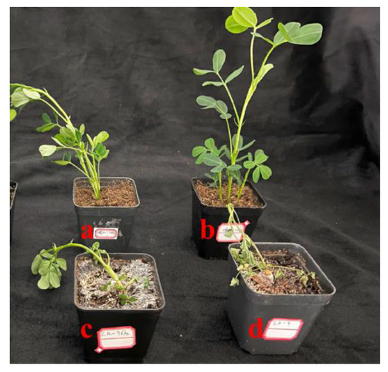
Figure 1.
Experimental potted plant for peanut southern blight. (a,b) Healthy, (c) mild, (d) severe.
2.2.2. Reflectance Spectral Measurement
The spectral measurement instrument of this experiment adopted the ASD Field Spec3 spectrometer and the matching plant probe to collect the spectral data of peanut leaves. The dimensions of the equipment are 12.7 cm × 36.8 cm × 29.2 cm and its weight is 5.44 kg. The wavelength range is 350–2500 nm, the sampling intervals are 1.4 nm (350–1000 nm) and 2 nm (1001–2500 nm), and the resampling interval is 1 nm. To avoid signal loss due to light absorption by atmospheric water vapor at wavelengths between 1400 nm and 1800 nm, the handheld Leaf Clip (ASD Leaf Clip) of the matching spectrometer was used to measure the spectrum of peanut leaves in this experiment. The built-in standard whiteboard was calibrated every 3 min to obtain a baseline close to 100% to ensure the accuracy of spectral data during the experiment.
2.3. Data Analysis Methods
2.3.1. Continuous Wavelet Transform
CWT is a linear operation that transforms a reflectance spectrum ( = 1, 2, …, n, where n is the number of spectral bands) into sets of coefficients at various scales by using a mother wavelet function. The mother wavelet is a small wave and has an average value of zero, which can be shifted (translated) and scaled (stretched or compressed) to produce a series of continuous wavelets as follows (dyadic numbers 21, 22, 23, …, 28 are denoted as Scale 1, Scale 2, Scale 3, …, Scale 8 for simplicity, respectively) [44]. In Formula (1), a represents the wavelength and represents the phase. After spectrum decomposition, the complete wavelet coefficient matrix of different bands and decomposition scales can be obtained:
where denotes the inner products of wavelets and the input spectrum. The output of a one-dimentional input spectrum comprises a two-dimentional wavelet power scalogram. Each element of the scalogram is a wavelet feature or wavelet coefficient that characterizes the correlation between a subset of the input spectrum and a scaled, shifted version of the mother wavelet [45].
The wavelet transform has proven to be an effective technique for extracting spectral information related to foliar chemistry and species composition from vegetation reflectance spectra when applied to spectroscopic data in remote sensing [46,47]. The Continuous Wavelet Transform (CWT) was utilized instead of the Discrete Wavelet Transform (DWT), because CWT provides scale components that are directly comparable to the input reflectance spectrum on a band-by-band basis, making the results easier to interpret.
2.3.2. Standard Normal Variable Transformation Processing
The SNV transformation was used to eliminate the influence of diffuse reflectance spectra caused by surface scattering and solid particle sizes during data collection. The average value of the spectral data was subtracted from the initial spectral reflectance data and then divided by its standard deviation [48]. The formula is as follows:
where , m is the total number of wavelengths, and = 1, 2…, .
2.3.3. Spectral Index
After reviewing the previous research on spectral indices, 12 spectral indices related to pest and disease stress were selected from the highly cited literature (Table 3). We then analyzed their weights using the relief algorithm to retain the most sensitive features for assessing their transferability.
Table 3.
The spectral indices included in this study.
2.3.4. Relief
The relief algorithm is a classic feature weight selection method that assigns weights to different features based on their relevance to the target variable.
In the initial feature set, the relief algorithm randomly selects a sample, denoted as “a”, and then searches for the nearest neighbor sample within the same class, known as the “Near Hit”. It also searches for the nearest neighbor sample outside the same class, referred to as the “Near Miss”. Feature weights are defined as follows: if the distance between the feature of interest and the Near Hit (H) is smaller than the distance between the same feature and the Near Miss (M), the weight is increased, which indicates that the feature effectively distinguishes different classes. Conversely, the weight is decreased for the reverse case [58].
where represents the distance between samples a and b for feature l, and and represent the upper and lower bounds of feature , respectively.
2.3.5. Machine Learning
In this study, three non-parametric machine learning algorithms, namely SVM, decision tree, and KNN, were employed to detect the severity of peanut southern blight.
The working principle of SVM is to create an optimal classification hyperplane using the training dataset and achieve different sample classifications based on minimal errors. In this study, we employed grid search to determine the best parameters, including the Radial Basis Function (RBF) kernel and polynomial kernel functions, for SVM classification [59]. Decision tree is a supervised learning algorithm that learns from a labeled training dataset to construct a root node and selects the best feature to further partition the data, aiming to achieve the best classification for each data point at each step [60]. KNN is a non-parametric classification method that assigns labels to data points based on the classification of K similar training samples. It does not assume any specific distribution for the data [61].
2.3.6. Evaluation of Accuracy
In this study, a 5-fold cross-validation with 100 repetitions was performed to evaluate the accuracy and robustness of all models. The first two sets of data (n = 122) were used to build and validate the models, while the third set of data (n = 53) was used for independent validation. The sample sizes for each severity level were approximately balanced across the three sets. The OA and kappa coefficient were used to assess the performance of the models. The formulas for calculating these two metrics are shown as Equations (6) and (7), respectively. In the equations, N represents the total number of classes; n represents the number of samples; represents the number of correctly classified samples; represents the diagonal elements of the confusion matrix; and represents each element of the confusion matrix.
3. Results
3.1. Spectral Response of Peanut Southern Blight
The sample contained 175 healthy, mild, moderate, and severe peanut leaves. The average spectral responses of each leaf type in different wavelength bands are shown in Figure 2. The findings indicate that in the green-light wavelength band (530–580 nm), healthy leaves exhibited the highest reflectance, while severely affected leaves showed the lowest reflectance. In the red-light wavelength band (620–670 nm), although the differences were not significant, some features were observed. Specifically, the spectral reflectance followed the pattern of healthy leaves > mild leaves > severe leaves, with a relatively small peak at 640 nm. In the red-edge wavelength band (700–780 nm), there were significant differences between healthy and severely affected leaves. The reason for this difference is attributed to the destruction of photosynthetic pigments, including chlorophyll, in infected leaves. The absorption capacity in the blue-light wavelength band (centered at 450 nm) and red-light wavelength band (centered at 660 nm) weakened, resulting in relatively small peaks. As chlorophyll continued to be destroyed and the photosynthetic ability weakened, the reflectance in the green-light wavelength band (centered at 550 nm) decreased, with a noticeable difference at 560 nm, due to changes in cell structure, loss of water content, and a decrease in chlorophyll and photosynthetic intensity in leaf cells caused by the continuous invasion of Sclerotium rolfsii in the intercellular space of the leaves. The hyperspectral reflectance of southern blight was relatively low in the visible band (400–760 nm) and relatively high in the near-infrared band (760–1350 nm). In comparison with healthy plants, the red edge of the infected southern blight largely shifted toward shorter wavelengths, indicating a “blue shift” phenomenon. In the overall analysis, the spectral reflectance of infected leaves in the visible light and near-infrared wavelength bands showed a decreasing trend with the increasing severity of the disease.
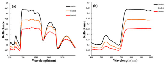
Figure 2.
Spectral characteristics of leaves of southern blight with different disease degrees: (a) 350–2500 nm; (b) 400–1000 nm.
3.2. Continuous-Wavelet-Transform-Sensitive Spectral Characterization
The spectral reflectance data of different severity levels collected in 2021 and 2022 were applied to CWT, and then the spectral results for each severity level were averaged, as shown in Figure 3b. Compared to the original spectra, CWT amplified the spectral differences in the red-edge range (700–790 nm) for different severity levels. Furthermore, we generated a classification scale based on the data, as shown in Figure 3a. We evaluated the accuracy of the machine learning models by incorporating the most sensitive wavelet features for each scale separately. Ultimately, we found that the SVM model using CWT (WF770~780, 5) performed best. The validation set OA was 90.5% and the kappa coefficient was 0.87 (Table 4).
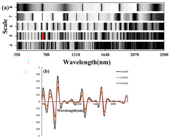
Figure 3.
(a) The X-axis represents the spectral wavelength range from 350 to 2500 nm, and the Y-axis represents the fourth to eighth wavelet scales. The grayscale brightness in the scale chart indicates the magnitude of classification accuracy (brighter indicates higher accuracy). The red region corresponds to the top 1% of the highest accuracy achieved. (b) CWT spectral curve.
Table 4.
Accuracy evaluation using CWT machine learning models.
3.3. Standard Normal Variable Transformation Processing
Figure 4 shows the spectral curves after SNV preprocessing, which altered the shape of the spectra compared to the original spectra (OR). SNV increased the separability of the spectral curves for different severity levels in the range of 350–1200 nm. We employed simple Linear Discriminant Analysis (LDA) to explore the sensitive bands of OR and SNV. For OR, the 940–1300 nm range exhibited the best performance, with the 942 nm band having the highest accuracy and an OA of 87.4%. For SNV, the 780–1300 nm range demonstrated the best performance, with the 903 nm band having the highest accuracy and an OA of 88.7%. Overall, both OR and SNV showed their highest accuracies in the near-infrared (NIR) range, and SNV enhanced NIR spectral differences among different severity levels (Figure 5).
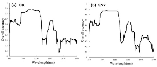
Figure 4.
Analysis of spectral separability based on Linear Discriminant Analysis. (a) Original spectrum, (b) SNV spectrum.
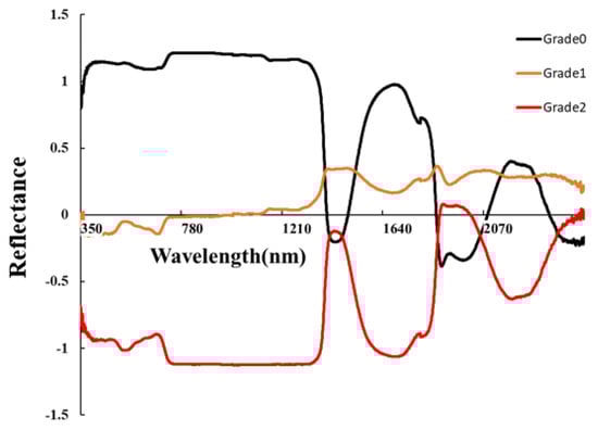
Figure 5.
SNV spectral curve.
3.4. Assessing the Transferability of Spectral Indices
To explore the spectral indices characterizing the severity of peanut southern blight, we analyzed the weights of 12 spectral indices using the relief algorithm (Figure 6a). To further evaluate the accuracy of these features, we performed the SVM modeling with different combinations of the features and evaluated their performance, as shown in Figure 6b. The highest OA was 74.9%, which was achieved by using 11 features. Notably, these features exhibited complementarity in the model. Removing the NSRI feature resulted in a 2.9% reduction in OA when the remaining 10 features were used. Likewise, removing the HI feature resulted in a 5.7% drop in OA when using the remaining nine features. Removing the G feature resulted in a 2.9% reduction in OA when using the remaining four features. Finally, removing the SIPI features led to a 2.9% decrease in OA. Based on these findings, we can conclude that the NSRI, HI, G, and SIPI features had a particular impact on the performance of the model.
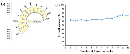
Figure 6.
(a) Weights of VIS; (b) plot of OA of VIS-superimposed SVM model.
We further conducted an autocorrelation analysis on the four selected features (Table 5). The correlation between each feature was found to be very low, indicating the absence of multicollinearity among the features. We proceeded to evaluate the accuracy of different machine learning models (Table 6). Among them, the SVM model achieved the highest performance on the training set, with an OA of 92.6% and kappa coefficient of 0.89. However, when applied to the independent validation data, the SVM model showed lower performance, with an OA of only 62.3% and kappa coefficient of 0.43, indicating poor robustness of the model.
Table 5.
Correlation analysis of NSRI, HI, G, and SIPI.
Table 6.
Accuracy of different machine learning models.
4. Discussion
4.1. Spectral Response Mechanism of Peanut Southern Blight
Peanut southern blight is a highly contagious and extremely destructive soil-borne fungal disease that occurs in most countries. It has become a key factor limiting peanut yield and quality [62,63]. Currently, there are few reports on the spectral response mechanism of peanut southern blight. In this study, we obtained spectral curves of samples with different severity levels through variable-controlled experiments. Machine learning techniques have been applied to hyperspectral data to enhance the detection capability of peanut southern blight severity. The main focus in this regard is to explore the spectral response of southern blight and obtain the optimal spectral features. These methods are consistent with previous advancements in the field [64].
Previous research has indicated that when plants are under stress from pests and diseases, their spectra tend to shift toward shorter wavelengths, and the amplitude of the red edge decreases [65]. When peanut plants are infected with southern blight disease, their photosynthesis is disrupted, resulting in a decrease in the absorption capacity of blue- and red-light wavelengths and a decrease in reflectance. As the disease progresses over time, it further damages the leaf structure, leading to the loss of chlorophyll and water content. Therefore, samples with different severity levels exhibit significant differences in the red-edge and near-infrared range (725–1200 nm). Infected samples generally show a decreasing trend in spectral reflectance, accompanied by a red-edge shift toward shorter wavelengths.
4.2. Advantages of Wavelet Analysis in Pest and Disease Detection
CWT can perform spectral decomposition at continuous wavelengths and scales. It effectively reduces noise interference, amplifies implicit weak spectral information, and plays a significant role in eliminating spectral background differences. Moreover, it enhances the sensitivity of spectra to the severity of peanut southern blight disease [66,67].
In this study, we conducted a comparative analysis using CWT at different scales, and the results showed that CWT at five scales achieved the best performance. Additionally, we found that the SVM model constructed using CWT (WF770~780, 5) outperformed the models based on the SNV and the original spectra. The main reason for this improvement is that CWT enhances the spectral response in the red-edge region, enabling effective differentiation of different severity levels of peanut southern blight disease [68].
4.3. Application of Spectral Index in Pest and Disease Detection
To assess the transferability of spectral indices under previous disease and pest stress, this study selected 12 spectral indices that contain information in the red-edge region. These indices were chosen based on current reports on the remote sensing of diseases and pests, such as wheat stripe rust [69] and apple fire blight [70]. Furthermore, relief analysis was employed to determine feature weights, and SVM models were evaluated by individually incorporating each feature. We observed that the model’s accuracy significantly changed when certain features were removed (Figure 6). This variation can be attributed to the complementary nature of different features in the model. As a result, we identified and confirmed four features as the final inputs for the model.
Although the SVM model achieved the highest accuracy on the training dataset, we observed poor robustness when validating the model using independent data. This may be attributed to the fact that the data from the final period were collected in spring, while the training dataset consisted of data collected in winter (Table 1). The different growth stages could have led to suboptimal model performance. However, we also identified several spectral indices that are related to the severity of peanut southern blight, indicating that spectral indices can rapidly detect the stress of plant diseases and pests, which is consistent with previous findings. Moving forward, our future work will likely focus on exploring additional vegetation indices that can accurately detect the severity of peanut southern blight, thus providing feasibility analysis for large-scale remote sensing of this disease.
4.4. Implications for Future Applications
The study also found some complex challenges in the early monitoring of peanut southern blight. The first problem is that the physiological interaction between fungal pathogens and host plants depends on pathogenic fungi. So, more in-depth investigation is needed to explore the interaction between different pathogens. Previously unconsidered variations can be revealed as the original source of reflectance data. A non-imaging sensor, to capture the average of healthy and diseased plant tissue parts, has been used to measure the reflectance curve, which causes many typical single-point measurement problems [71]. The second challenge lies in the complexity of field environments, where phenomena like spectral variations from the same object and the co-occurrence of multiple diseases can occur. Our severity classification model for peanut southern blight built at the leaf scale may be influenced by various factors. For example, in terms of spectral response, peanut leaf spot disease shows a significant negative correlation between the disease index and the spectral curve in the NIR range, which is very similar to the spectral response of peanut southern blight [11]. In terms of plant structure, peanut stem rot disease also exhibits yellowish-brown rotting signs at the base of the stem during the early stages of infection [72]. However, without the presence of white mycelium and brown sclerotia at the base, it can often lead to misinterpretation. Therefore, it requires the integration of field meteorological data, agronomic background, and other relevant data for comprehensive discrimination, which is a difficult task. The third challenge is to integrate multiple data sources and enable data sharing of peanut southern blight between different provinces, aiming to improve the model’s transferability. Our future focus is on integrating multi-source remote sensing data to achieve data exchange between provinces and establishing a dynamic monitoring platform for peanut southern blight. This platform aims to provide technical support for disease prevention and control in peanuts.
5. Conclusions
This study analyzed the spectral response mechanism of different severity levels of peanut southern blight. For the severity classification problem, we compared the machine learning modeling using CWT with traditional spectral indices and spectral preprocessing methods. The results showed that CWT was more effective and amplified the spectral differences between different levels of severity. Furthermore, this study emphasized the potential of using hyperspectral sensors for monitoring peanut southern blight, which is an exciting tool for disease management and control in peanuts.
Author Contributions
W.G.: conceptualization, methodology, writing—original draft. H.S.: methodology, writing—review and editing. H.Q.: methodology, investigation, supervision. H.Z.: data curation, methodology. L.Z.: materials and methods. P.D.: data curation, methodology. X.S.: methodology, investigation, conceptualization. All authors have read and agreed to the published version of the manuscript.
Funding
This research was funded by The Henan Provincial Science and Technology Major Project (221100110100); National Natural Science Foundation of China, grant number (32271993); The Joint Fund of Science and Technology Research Development program (Cultivation project of preponderant discipline) of Henan Province, China (222301420114).
Data Availability Statement
Not applicable.
Conflicts of Interest
The authors declare no conflict of interest.
References
- Avijit, T.; Swaroopa, R.T.; Sharath, C.U.S.; Raju, G.; Chobe, D.R.; Mamta, S. Exploring Combined Effect of Abiotic (Soil Moisture) and Biotic (Sclerotium rolfsii Sacc.) Stress on Collar Rot Development in Chickpea. Front. Plant Ence 2018, 9, 1154. [Google Scholar]
- Thiessen, L.D.; Woodward, J.E. Diseases of peanut caused by soilborne pathogens in the Southwestern United States. Int. Sch. Res. Not. 2012, 2012, 1–9. [Google Scholar] [CrossRef]
- Xu, M.; Zhang, X.; Yu, J.; Guo, Z.; Wan, S. Biological control of peanut southern blight (Sclerotium rolfsii) by the strain Bacillus pumilus LX11. Biocontrol Sci. Technol. 2020, 30, 485–489. [Google Scholar] [CrossRef]
- Zhang, W.; Zhang, B.-W.; Deng, J.-F.; Li, L.; Yi, T.-Y.; Hong, Y.-Y. The resistance of peanut to soil-borne pathogens improved by rhizosphere probiotics under calcium treatment. BMC Microbiol. 2021, 21, 299. [Google Scholar] [CrossRef] [PubMed]
- Zhang, J.; Huang, Y.; Pu, R.; Gonzalez-Moreno, P.; Yuan, L.; Wu, K.; Huang, W. Monitoring plant diseases and pests through remote sensing technology: A review. Comput. Electron. Agric. 2019, 165, 104943. [Google Scholar] [CrossRef]
- Long, T.; Bowen, X.; Ziyi, W.; Dong, L.; Xia, Y.; Qiang, C.; Yan, Z.; Weixing, C.; Tao, C. Spectroscopic detection of rice leaf blast infection from asymptomatic to mild stages with integrated machine learning and feature selection. Remote Sens. Environ. 2021, 257, 112350. [Google Scholar]
- Zhang, N.; Yang, G.; Pan, Y.; Yang, X.; Chen, L.; Zhao, C. A Review of Advanced Technologies and Development for Hyperspectral-Based Plant Disease Detection in the Past Three Decades. Remote Sens. 2020, 12, 3188. [Google Scholar] [CrossRef]
- Feng, L.; WU, D.; HE, Y. Identification and classification of rice leaf blast based on multi-spectral imaging sensor. Spectrosc. Spectr. Anal. 2009, 29, 2730–2733. [Google Scholar]
- Zhou, L.-N.; Yu, H.-Y.; Zhang, L.; Ren, S.; Sui, Y.-Y.; Yu, L.-J. Rice blast prediction model based on analysis of chlorophyll fluorescence spectrum. Spectrosc. Spectr. Anal. 2014, 34, 1003–1006. [Google Scholar]
- Huang, W.; Guan, Q.; Luo, J.; Zhang, J.; Zhao, J.; Liang, D.; Huang, L.; Zhang, D. New optimized spectral indices for identifying and monitoring winter wheat diseases. IEEE J. Sel. Top. Appl. Earth Obs. Remote Sens. 2014, 7, 2516–2524. [Google Scholar] [CrossRef]
- Chen, T.; Zhang, J.; Chen, Y.; Wan, S.; Zhang, L. Detection of peanut leaf spots disease using canopy hyperspectral reflectance. Comput. Electron. Agric. 2019, 156, 677–683. [Google Scholar] [CrossRef]
- Jiang, X.; Zhen, J.; Miao, J.; Zhao, D.; Shen, Z.; Jiang, J.; Gao, C.; Wu, G.; Wang, J. Newly-developed three-band hyperspectral vegetation index for estimating leaf relative chlorophyll content of mangrove under different severities of pest and disease. Ecol. Indic. 2022, 140, 108978. [Google Scholar] [CrossRef]
- Talbot, N.J. On the trail of a cereal killer: Exploring the biology of Magnaporthe grisea. Annu. Rev. Microbiol. 2003, 57, 177–202. [Google Scholar] [CrossRef]
- Baranoski, G.; Rokne, J. A practical approach for estimating the red edge position of plant leaf reflectance. Int. J. Remote Sens. 2005, 26, 503–521. [Google Scholar] [CrossRef]
- Ray, S.S.; Jain, N.; Arora, R.; Chavan, S.; Panigrahy, S. Utility of hyperspectral data for potato late blight disease detection. J. Indian Soc. Remote Sens. 2011, 39, 161–169. [Google Scholar] [CrossRef]
- Sathish, C.; Nakhawa, A.; Bharti, V.S.; Jaiswar, A.; Deshmukhe, G. Estimation of extent of the mangrove defoliation caused by insect Hyblaea puera (Cramer, 1777) around Dharamtar creek, India using Sentinel 2 images. Reg. Stud. Mar. Sci. 2021, 48, 102054. [Google Scholar] [CrossRef]
- Wang, H.-G.; Ma, Z.-H.; Wang, T.; Cai, C.-J.; An, H.; Zhang, L.-D. Application of hyperspectral data to the classification and identification of severity of wheat stripe rust. Guang Pu Xue Yu Guang Pu Fen Xi = Guang Pu 2007, 27, 1811–1814. [Google Scholar]
- He, R.; Li, H.; Qiao, X.; Jiang, J. Using wavelet analysis of hyperspectral remote-sensing data to estimate canopy chlorophyll content of winter wheat under stripe rust stress. Int. J. Remote Sens. 2018, 39, 4059–4076. [Google Scholar] [CrossRef]
- Yang, Y.; Chai, R.; He, Y. Early detection of rice blast (Pyricularia) at seedling stage in Nipponbare rice variety using near-infrared hyper-spectral image. Afr. J. Biotechnol. 2012, 11, 6809–6817. [Google Scholar] [CrossRef]
- Feng, Z.; Guan, H.; Yang, T.; He, L.; Duan, J.; Song, L.; Wang, C.; Feng, W. Estimating the canopy chlorophyll content of winter wheat under nitrogen deficiency and powdery mildew stress using machine learning. Comput. Electron. Agric. 2023, 211, 107989. [Google Scholar] [CrossRef]
- Hernández-Clemente, R.; Hornero, A.; Mottus, M.; Peñuelas, J.; González-Dugo, V.; Jiménez, J.; Suárez, L.; Alonso, L.; Zarco-Tejada, P.J. Early diagnosis of vegetation health from high-resolution hyperspectral and thermal imagery: Lessons learned from empirical relationships and radiative transfer modelling. Curr. For. Rep. 2019, 5, 169–183. [Google Scholar] [CrossRef]
- Berger, K.; Machwitz, M.; Kycko, M.; Kefauver, S.C.; Van Wittenberghe, S.; Gerhards, M.; Verrelst, J.; Atzberger, C.; van der Tol, C.; Damm, A. Multi-sensor spectral synergies for crop stress detection and monitoring in the optical domain: A review. Remote Sens. Environ. 2022, 280, 113198. [Google Scholar] [CrossRef] [PubMed]
- Feret, J.-B.; François, C.; Asner, G.P.; Gitelson, A.A.; Martin, R.E.; Bidel, L.P.; Ustin, S.L.; Le Maire, G.; Jacquemoud, S. PROSPECT-4 and 5: Advances in the leaf optical properties model separating photosynthetic pigments. Remote Sens. Environ. 2008, 112, 3030–3043. [Google Scholar] [CrossRef]
- Al-Saddik, H.; Laybros, A.; Billiot, B.; Cointault, F. Using image texture and spectral reflectance analysis to detect Yellowness and Esca in grapevines at leaf-level. Remote Sens. 2018, 10, 618. [Google Scholar] [CrossRef]
- Verrelst, J.; Camps-Valls, G.; Muñoz-Marí, J.; Rivera, J.P.; Veroustraete, F.; Clevers, J.G.; Moreno, J. Optical remote sensing and the retrieval of terrestrial vegetation bio-geophysical properties–A review. ISPRS J. Photogramm. Remote Sens. 2015, 108, 273–290. [Google Scholar] [CrossRef]
- Calderón, R.; Navas-Cortés, J.A.; Lucena, C.; Zarco-Tejada, P.J. High-resolution airborne hyperspectral and thermal imagery for early detection of Verticillium wilt of olive using fluorescence, temperature and narrow-band spectral indices. Remote Sens. Environ. 2013, 139, 231–245. [Google Scholar] [CrossRef]
- Meena, S.V.; Dhaka, V.S.; Sinwar, D. Exploring the Role of Vegetation Indices in Plant Diseases Identification. In Proceedings of the 2020 Sixth International Conference on Parallel, Distributed and Grid Computing (PDGC), Solan, India, 6–8 November 2020; pp. 372–377. [Google Scholar]
- Zhao, H.; Yang, C.; Guo, W.; Zhang, L.; Zhang, D. Automatic estimation of crop disease severity levels based on vegetation index normalization. Remote Sens. 2020, 12, 1930. [Google Scholar] [CrossRef]
- Fu, H.; Zhao, H.; Song, R.; Yang, Y.; Li, Z.; Zhang, S. Cotton aphid infestation monitoring using Sentinel-2 MSI imagery coupled with derivative of ratio spectroscopy and random forest algorithm. Front. Plant Sci. 2022, 13, 1029529. [Google Scholar] [CrossRef]
- Huang, W.; Lu, J.; Ye, H.; Kong, W.; Mortimer, A.H.; Shi, Y. Quantitative identification of crop disease and nitrogen-water stress in winter wheat using continuous wavelet analysis. Int. J. Agric. Biol. Eng. 2018, 11, 145–152. [Google Scholar] [CrossRef]
- Cheng, T.; Riaño, D.; Ustin, S.L. Detecting diurnal and seasonal variation in canopy water content of nut tree orchards from airborne imaging spectroscopy data using continuous wavelet analysis. Remote Sens. Environ. 2014, 143, 39–53. [Google Scholar] [CrossRef]
- Blackburn, G.A.; Ferwerda, J.G. Retrieval of chlorophyll concentration from leaf reflectance spectra using wavelet analysis. Remote Sens. Environ. 2007, 112, 1614–1632. [Google Scholar] [CrossRef]
- Rivard, B.; Feng, J.; Gallie, A.; Sanchez-Azofeifa, A. Continuous wavelets for the improved use of spectral libraries and hyperspectral data. Remote Sens. Environ. 2008, 112, 2850–2862. [Google Scholar] [CrossRef]
- Ampe, E.M.; Hestir, E.L.; Bresciani, M.; Salvadore, E.; Brando, V.E.; Dekker, A.G.; Malthus, T.J.; Jansen, M.; Triest, L.; Batelaan, O. A Wavelet Approach for Estimating Chlorophyll-A From Inland Waters with Reflectance Spectroscopy. IEEE Geosci. Remote Sens. Lett. 2014, 11, 89–93. [Google Scholar] [CrossRef]
- Juhua, L.; Wenjiang, H.; Jinling, Z.; Jingcheng, Z.; Chunjiang, Z.; Ronghua, M. Detecting Aphid Density of Winter Wheat Leaf Using Hyperspectral Measurements. IEEE J. Sel. Top. Appl. Earth Obs. Remote Sens. 2013, 6, 690–698. [Google Scholar]
- Pu, R.; Gong, P. Wavelet transform applied to EO-1 hyperspectral data for forest LAI and crown closure mapping. Remote Sens. Environ. 2004, 91, 212–224. [Google Scholar] [CrossRef]
- Banskota, A.; Wynne, R.H.; Kayastha, N. Improving within-genus tree species discrimination using the discrete wavelet transform applied to airborne hyperspectral data. Int. J. Remote Sens. 2011, 32, 3551–3563. [Google Scholar] [CrossRef]
- Asaari, M.S.M.; Mishra, P.; Mertens, S.; Dhondt, S.; Wuyts, N.; Scheunders, P. Close-range hyperspectral image analysis for the early detection of plant stress responses in individual plants in a high-throughput phenotyping platform. ISPRS J. Photogramm. Remote Sens. 2018, 138, 121–138. [Google Scholar] [CrossRef]
- Feng, Z.; Zhang, H.; Duan, J.; He, L.; Yuan, X.; Gao, Y.; Liu, W.; Li, X.; Feng, W. Improved Spectral Detection of Nitrogen Deficiency and Yellow Mosaic Disease Stresses in Wheat Using a Soil Effect Removal Algorithm and Machine Learning. Remote Sens. 2023, 15, 2513. [Google Scholar] [CrossRef]
- Feng, Z.; Song, L.; Duan, J.; He, L.; Zhang, Y.; Wei, Y.; Feng, W. Monitoring wheat powdery mildew based on hyperspectral, thermal infrared, and RGB image data fusion. Sensors 2022, 22, 31. [Google Scholar] [CrossRef]
- Hamed, A.M.S.; Mehdi, M.; Asghari, B.B. A feature extraction method based on spectral segmentation and integration of hyperspectral images. Int. J. Appl. Earth Obs. Geoinf. 2019, 89, 102097. [Google Scholar]
- Wang, H.; Li, G.; Ma, Z.; Li, X. Image recognition of plant diseases based on backpropagation networks. In Proceedings of the 2012 5th International Congress on Image and Signal Processing, Agadir, Morocco, 28–30 June 2012; pp. 894–900. [Google Scholar]
- Kononenko, I. Estimating attributes: Analysis and extensions of RELIEF. In Proceedings of the European conference on machine learning, Catania, Italy, 6–8 April 1994; pp. 171–182. [Google Scholar]
- Bruce, L.M.; Li, J.; Huang, Y. Automated detection of subpixel hyperspectral targets with adaptive multichannel discrete wavelet transform. IEEE Trans. Geosci. Remote Sens. 2002, 40, 977–980. [Google Scholar] [CrossRef]
- Bruce, L.M.; Li, J. Wavelets for computationally efficient hyperspectral derivative analysis. IEEE Trans. Geosci. Remote Sens. 2001, 39, 1540–1546. [Google Scholar] [CrossRef]
- Blackburn, G.A. Wavelet decomposition of hyperspectral data: A novel approach to quantifying pigment concentrations in vegetation. Int. J. Remote Sens. 2007, 28, 2831–2855. [Google Scholar] [CrossRef]
- Cheng, T.; Rivard, B.; Sánchez-Azofeifa, A. Spectroscopic determination of leaf water content using continuous wavelet analysis. Remote Sens. Environ. 2010, 115, 659–670. [Google Scholar] [CrossRef]
- Dhanoa, M.; Lister, S.; Sanderson, R.; Barnes, R. The link between multiplicative scatter correction (MSC) and standard normal variate (SNV) transformations of NIR spectra. J. Near Infrared Spectrosc. 1994, 2, 43–47. [Google Scholar] [CrossRef]
- Penuelas, J.; Baret, F.; Filella, I. Semi-empirical indices to assess carotenoids/chlorophyll a ratio from leaf spectral reflectance. Photosynthetica 1995, 31, 221–230. [Google Scholar]
- Gitelson, A.; Yacobi, Y.; Schalles, J.; Rundquist, D.; Han, L.; Stark, R.; Etzion, D. Remote estimation of phytoplankton density in productive waters. Adv. Limnol. Stuttg. 2000, 55, 121–136. [Google Scholar]
- Mahlein, A.-K.; Rumpf, T.; Welke, P.; Dehne, H.-W.; Plümer, L.; Steiner, U.; Oerke, E.-C. Development of spectral indices for detecting and identifying plant diseases. Remote Sens. Environ. 2013, 128, 21–30. [Google Scholar] [CrossRef]
- Ferwerda, J.G.; Skidmore, A.K.; Mutanga, O. Nitrogen detection with hyperspectral normalized ratio indices across multiple plant species. Int. J. Remote Sens. 2005, 26, 4083–4095. [Google Scholar] [CrossRef]
- Peñuelas, J.; Pinol, J.; Ogaya, R.; Filella, I. Estimation of plant water concentration by the reflectance water index WI (R900/R970). Int. J. Remote Sens. 1997, 18, 2869–2875. [Google Scholar] [CrossRef]
- Sims, D.A.; Gamon, J.A. Relationships between leaf pigment content and spectral reflectance across a wide range of species, leaf structures and developmental stages. Remote Sens. Environ. 2002, 81, 337–354. [Google Scholar] [CrossRef]
- Liu, L.-Y.; Huang, W.-J.; Pu, R.-L.; Wang, J.-H. Detection of internal leaf structure deterioration using a new spectral ratio index in the near-infrared shoulder region. J. Integr. Agric. 2014, 13, 760–769. [Google Scholar] [CrossRef]
- Merzlyak, M.N.; Gitelson, A.A.; Chivkunova, O.B.; Rakitin, V.Y. Non-destructive optical detection of pigment changes during leaf senescence and fruit ripening. Physiol. Plant. 1999, 106, 135–141. [Google Scholar] [CrossRef]
- Blackburn, G.A. Spectral indices for estimating photosynthetic pigment concentrations: A test using senescent tree leaves. Int. J. Remote Sens. 1998, 19, 657–675. [Google Scholar] [CrossRef]
- Urbanowicz, R.J.; Meeker, M.; La Cava, W.; Olson, R.S.; Moore, J.H. Relief-based feature selection: Introduction and review. J. Biomed. Inform. 2018, 85, 189–203. [Google Scholar] [CrossRef]
- Cortes, C.; Vapnik, V. Support-vector networks. Mach. Learn. 1995, 20, 273–297. [Google Scholar] [CrossRef]
- Rokach, L.; Maimon, O. Decision trees. In Data Mining and Knowledge Discovery Handbook; Springer: New York, NY, USA, 2005; pp. 165–192. [Google Scholar]
- Guo, G.; Wang, H.; Bell, D.; Bi, Y.; Greer, K. KNN model-based approach in classification. In Proceedings of the On the Move to Meaningful Internet Systems 2003: CoopIS, DOA, and ODBASE: OTM Confederated International Conferences, CoopIS, DOA, and ODBASE 2003, Catania, Italy, 3–7 November 2003; pp. 986–996. [Google Scholar]
- Zhiyuan, H.; Kaidi, C.; Mengke, W.; Chaofan, J.; Te, Z.; Meizi, W.; Pengqiang, D.; Leiming, H.; Lin, Z. Bioactivity of the DMI fungicide mefentrifluconazole against Sclerotium rolfsii, the causal agent of peanut southern blight. Pest Manag. Sci. 2023, 79, 2126–2134. [Google Scholar]
- Damicone, J.; Jackson, K. Factors affecting chemical control of southern blight of peanut in Oklahoma. Plant Dis. 1994, 78, 482–486. [Google Scholar] [CrossRef]
- Rumpf, T.; Mahlein, A.-K.; Steiner, U.; Oerke, E.-C.; Dehne, H.-W.; Plümer, L. Early detection and classification of plant diseases with support vector machines based on hyperspectral reflectance. Comput. Electron. Agric. 2010, 74, 91–99. [Google Scholar] [CrossRef]
- Jiang, J.-B.; Chen, Y.-H.; Huang, W.-J. Using the distance between hyperspectral red edge position and yellow edge position to identify wheat yellow rust disease. Spectrosc. Spectr. Anal. 2010, 30, 1614–1618. [Google Scholar]
- Zhang, J.-C.; Lin, Y.; Wang, J.-H.; Huang, W.-J.; Chen, L.-P.; Zhang, D.-Y. Spectroscopic leaf level detection of powdery mildew for winter wheat using continuous wavelet analysis. J. Integr. Agric. 2012, 11, 1474–1484. [Google Scholar] [CrossRef]
- Zhang, J.; Pu, R.; Loraamm, R.W.; Yang, G.; Wang, J. Comparison between wavelet spectral features and conventional spectral features in detecting yellow rust for winter wheat. Comput. Electron. Agric. 2014, 100, 79–87. [Google Scholar] [CrossRef]
- Li, D.; Cheng, T.; Zhou, K.; Zheng, H.; Yao, X.; Tian, Y.; Zhu, Y.; Cao, W. WREP: A wavelet-based technique for extracting the red edge position from reflectance spectra for estimating leaf and canopy chlorophyll contents of cereal crops. ISPRS J. Photogramm. Remote Sens. 2017, 129, 103–117. [Google Scholar] [CrossRef]
- Yao, Z.; Lei, Y.; He, D. Early visual detection of wheat stripe rust using visible/near-infrared hyperspectral imaging. Sensors 2019, 19, 952. [Google Scholar] [CrossRef]
- Xiao, D.; Pan, Y.; Feng, J.; Yin, J.; Liu, Y.; He, L. Remote sensing detection algorithm for apple fire blight based on UAV multispectral image. Comput. Electron. Agric. 2022, 199, 107137. [Google Scholar] [CrossRef]
- Scholten, J.; Klein, M.; Steemers, A.; de Bruin, G. Hyperspectral imaging-A Novel non-destructive analytical tool in paper and writing durability research. In Proceedings of the Art ‘05–8th International Conference on Non-Destructive Investigations and Microanalysis for the Diagnostics and Conservation of the Cultural and Environmental Heritage, Lecce, Italy, 15–19 May 2005. [Google Scholar]
- Timper, P.; Minton, N.; Johnson, A.; Brenneman, T.; Culbreath, A.; Burton, G.; Baker, S.; Gascho, G. Influence of cropping systems on stem rot (Sclerotium rolfsii), Meloidogyne arenaria, and the nematode antagonist Pasteuria penetrans in peanut. Plant Dis. 2001, 85, 767–772. [Google Scholar] [CrossRef]


Disclaimer/Publisher’s Note: The statements, opinions and data contained in all publications are solely those of the individual author(s) and contributor(s) and not of MDPI and/or the editor(s). MDPI and/or the editor(s) disclaim responsibility for any injury to people or property resulting from any ideas, methods, instructions or products referred to in the content. |
© 2023 by the authors. Licensee MDPI, Basel, Switzerland. This article is an open access article distributed under the terms and conditions of the Creative Commons Attribution (CC BY) license (https://creativecommons.org/licenses/by/4.0/).