Abstract
This study aimed to investigate how the combination of texture information and spectral index affects the accuracy of the soil salinity inversion model. Taking the Bianwan Farm in Jiuquan City, Gansu Province, China as the research area, the multi-spectral data and soil salinity data at 0–15 cm, 15–30 cm and 30–50 cm depths in the sampling area under alfalfa coverage were collected, and spectral reflectance and texture features were obtained from a multispectral image. Moreover, the red-edge band was introduced to improve the spectral index, and gray correlation analysis was utilized to screen sensitive features. Five types of alfalfa-covered soil salinity machine learning inversion models based on random forest (RF) and extreme learning machine (ELM) algorithms were constructed, using the salinity index (SIs), vegetation index (VIs), salinity index + vegetation index (SIs + VIs), vegetation index + texture feature (VIs + TFs), and vegetation index + texture index (VIs + TIs). The determination coefficient R2, root-mean-square error (RMSE) and mean absolute error (MAE) were used to evaluate each model’s performance. The results show that the VIs model is more accurate than the SIs and SIs +VIs models. Combining texture information with VIs improves the inversion accuracy, and the VIs + TIs model has the best inversion effect. From the perspective of inversion depth, the inversion effect for 0–15 cm soil salinity was significantly better than that for other depths, and was the best inversion depth under alfalfa cover. The average R2 of the RF model was 10% higher than that of the ELM. The RF algorithm has high inversion accuracy and stability and performs better than ELM. These findings can serve as a theoretical basis for the efficient inversion of soil salinity and management of saline–alkali lands.
1. Introduction
Soil salinization is one of the most urgent soil problems worldwide, leading to the degradation of cultivated land and reduced crop yield on a large scale [1]. With a global saline–alkali soil area of about 833 million hectares, about 1.5 billion people face a significant challenge to food security [2]. Soil salt content plays a vital role in crop yield and growth [3]. Exploring the rapid inversion of soil salinity at different depths under crop coverage is of practical significance for developing agriculture and animal husbandry in saline–alkali areas. However, acquiring soil salt information mainly depends on field sampling and determination or a portable soil detector, which can be inefficient, involves limited samples, and requires cumbersome steps [4,5]. However, some researchers have found that soil salinity exhibits absorption peaks at 416 nm, 487 nm, 671 nm, and 905 nm wavebands [6]. The intensity of these absorption peaks has a significant correlation with the salinity content in soil, forming the basis for estimating soil salinity using spectral information. Remote sensing technology, capable of rapidly acquiring spectral information of large areas, has been widely used in monitoring soil salinization [7,8]. Among these, satellite remote sensing is often employed for large-scale irrigation area salinity research. Wang F [9] used Landsat-8 satellite images to predict soil salinity in the Kuqa Oasis, Xinjiang, China. Additionally, Abuzaid A.S. [10] tested the ability of Landsat 8 Operational Land Imager (OLI) data to retrieve soil salinity and sodicity during the wet and dry seasons in an arid landscape. Although these methods have yielded better results, overall, due to the low resolution of satellite images and various limiting factors such as climate and cloud cover, satellite imagery is not suitable for studying soil parameters at the field scale [11,12].
In contrast, unmanned aerial vehicles (UAVs) possess several advantages, including easy operation, short duration, high throughput, and high spatial and temporal resolution [13]. These advantages have greatly facilitated the development of precision and modern agriculture [14,15]. Furthermore, UAVs can be equipped with various imaging cameras for monitoring soil salinization. Zhu [16] combined UAV-based hyperspectral visible and near-infrared spectra with two feature selection techniques to predict soil salinity, validating the effectiveness of hyperspectral imagery in estimating and mapping surface soil salinity. Zhao [17] used a UAV-mounted multispectral camera to develop a model for quantifying soil salinity based on different vegetation cover, which provides a good reflection of actual soil salt content. Nevertheless, how to improve the accuracy of the inversion model remains a hot topic in current research.
The vegetation growth status has a strong correlation with the salinity value of the soil [18]. From the spectral perspective, this is manifested in two ways: on the one hand, it is reflected in the differences in spectral reflectance of crop leaves; on the other hand, the texture features of the spectral images themselves will also significantly differ due to the variations in soil salinity or leaf differences [19,20]. Existing research results show that these texture features have been widely used to estimate vegetation parameters [21,22,23], and satisfactory results have been obtained. It is considered that the combination of texture information and spectral information can significantly improve the accuracy of the model. However, the current process of soil salinity inversion using drones still mainly relies on spectral indices [24,25,26], and there are few reports on the inversion of soil salinity combining spectral information and image texture features.
Therefore, in order to improve the accuracy of the soil salinity inversion model of cultivated land and explore the applicability of spectral information and image texture features in the inversion of soil salinity, the soil at different depths under alfalfa coverage was taken as the research object, and the spectral index and texture features of UAV multi-spectral image were extracted to construct the soil salinity inversion model under various combinations of input. This study was designed to: (1) investigate how the combination of texture information and spectral index affects the accuracy of the inversion model; (2) determine the best soil salinity inversion model by assessing the accuracy of each model and (3) to identify the optimal soil salinity inversion depth beneath alfalfa coverage. The finding of this study can provide theoretical support for the rapid acquisition of soil salinity information in cultivated land.
2. Materials and Methods
2.1. Overview of the Study Area
Bianwan Farm, situated in the western region of the Hexi Corridor and belonging to Jiuquan City, Gansu Province, China (Figure 1a,b), covers an area of approximately 15.6 km2. The farm center is located at a longitude of 98°30′36″ E and latitude of 39°51′00″ N. The area is characterized by an arid continental climate with high solar radiation and a large disparity between evaporation and precipitation, resulting in perennial aridity. The average annual rainfall is 87 mm, and the average annual evaporation is 2140 mm. The main crops are alfalfa, wheat, corn, and onion.
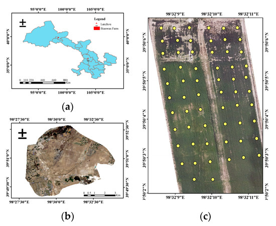
Figure 1.
Study area diagram. (a) Gansu province. (b) Bianwan Farm. (c) Soil sampling points of alfalfa plot.
2.2. Data Collection and Processing
2.2.1. UAV Multispectral Image
Alfalfa is a forage crop typically grown in arid saline–alkali areas, owing to its remarkable ability to withstand drought, barren conditions, and high salinity levels. Its short growth cycle and high yield make it essential to crop farmers and herdsmen in certain regions. In June 2022, at Bianwan Farm, UAV data were collected under sunny weather conditions with no rainfall and an average temperature of 33 °C. The experimental images were captured using the DJI Phantom 4, which comprises one color sensor for visible light imaging and five monochrome sensors (R, G, B, NIR, red edge) for multispectral imaging (Figure 2a). Each individual sensor has an effective pixel count of 2.08 million. The ISO range for the color sensor is 200–800. The specific wavelength information of the five monochromatic sensors is shown in Table 1. For instance, “450 nm (±16)” indicates that the blue spectral sensor’s filtering wavelength range is 434–466 nm. Finally, the photos obtained by the UAV are imported into DJI Terra for image correction, stitching and other preprocessing, and the multi-spectral image map for this study is obtained.
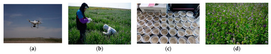
Figure 2.
Data collection and processing. (a) DJI Phantom 4 collects multi-spectral data. (b) Collect alfalfa-covered soil. (c) Measure the salt content of soil samples. (d) Alfalfa.

Table 1.
Multispectral camera parameters and UAV parameters.
2.2.2. Field Soil Salinity Data
Soil sampling was carried out in the alfalfa planting region at Bianwan Farm (Figure 2b). Sampling was conducted during a period where there was neither irrigation nor rainfall. During this time, the alfalfa in the sample area was fully flowering, with a height ranging from 40 to 80 cm (Figure 2d). A total of 62 sampling points were evenly distributed in the alfalfa plot, as demonstrated in Figure 1c. Soil samples were taken from three different depths, namely, 0–15 cm, 15–30 cm, and 30–50 cm, and location information for each point was recorded. Each soil sample, weighing 30 g, was placed in an aluminum box, dried, ground, and sieved with an aperture of 2 mm. To stir the sieved soil samples, 150 mL of distilled water was added [27]. After standing for 12 h, the conductivity of the soil solution (EC1:5, ms/cm) was determined using DJS-1C, and the soil salt content (SSC, %) was calculated using an empirical formula conversion [28] (Figure 2c).
2.3. Construct Spectral Index
The salinity index (SIs) is commonly used for the rapid assessment and inversion of soil salinization [29], and is highly correlated with soil salinity. There are 15 salinity indexes, including SI, SI1, SI2, SI3, S1, S2, S3, S4, S5, S6, SI-T, BI, NDSI, Int1, and Int2. The vegetation index (VIs), on the other hand, is used for qualitative and quantitative evaluations of vegetation growth and coverage [30]. A total of 16 common vegetation indexes are used, including RVI, NLI, IPVI, GLI, NDVI, NNIR, DVI, EVI, GCI, GSAVI, GRVI, GOSAVI, GNDVI, GDVI, LAI, and CI. For saline–alkali farmland covered with crops, the UAV multispectral camera cannot directly acquire the spectral reflectance of the soil surface. To enhance the accuracy of the inversion model, research suggests introducing the red-edge band, closely related to various physical and chemical parameters of the vegetation [31,32,33] and replacing the red band with the red-edge band to improve each index.
The grey relation analysis (GRA) is a method used to measure the correlation between elements. It is based on the similarity or dissimilarity of the development trend between the two elements. Specifically, the grey correlation degree is calculated based on the relationship between the trends of the two factors. If the trends are consistent, the correlation value is higher, and if they are inconsistent, it is lower [34]. Table 2 provides the order of grey correlation degree between the SIs and VIs. The Table clearly shows that the correlation degree of the improved index of the red-edge band and the measured salt content of the soil is particularly high. In order to minimize the influence of the number of screening indexes on the model, the first five indexes of correlation degree of each soil layer are selected to participate in the model construction. The calculation formula for the index is provided in Table 3, and the selected indexes of soil layers at different depths are basically the same.
Table 2.
Grey correlation value and ranking of soil salt content and SIs, VIs at different depths.
Table 3.
Calculation formula of spectral index.
2.4. Multispectral Image Texture Analysis
2.4.1. Texture Feature Extraction
The gray-level co-occurrence matrix (GLCM) is an image texture feature extraction method widely used in remote sensing [35,36,37]. However, due to the large amount of data in the matrix, it is not directly used to distinguish textures. Instead, some statistics based on it are used as texture classification features. This study used the co-occurrence measures window of ENVI 5.3.1 to extract the mean, variance, homogeneity, contrast, dissimilarity, entropy, second moment, and correlation of each band of the UAV multispectral image. The texture features of the visible light image are depicted in Figure 3.
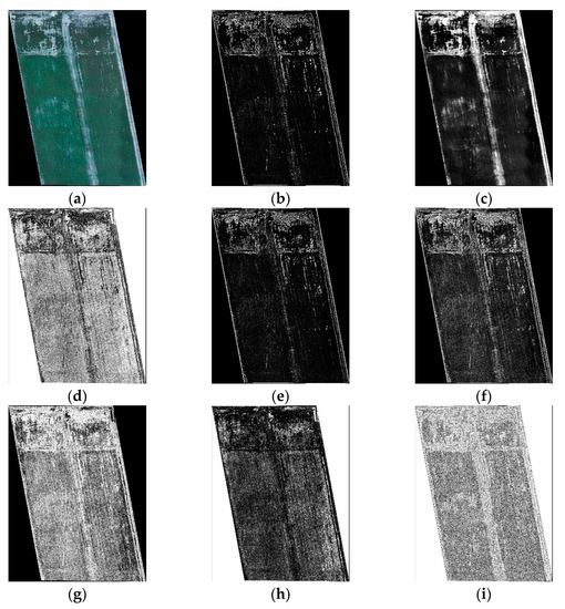
Figure 3.
Texture features of visible light image. (a) Visible light image. (b) Mean. (c) Variance. (d) Homogeneity. (e) Contrast. (f) Dissimilarity. (g) Entropy. (h) Second Moment. (i) Correlation.
2.4.2. Construct Texture Index
Figure 4 illustrates the analysis of the correlation between soil at different depths under alfalfa coverage and eight texture features of each spectral band. The correlations between the measured salt content at different depths and the texture features of each spectral band are low, with a correlation coefficient |r| < 0.39, making direct model construction impractical. On the other hand, the red and blue bands have a high response to soil salinization, with |r| above 0.50. Therefore, it is feasible to construct a texture index using 16 texture features of red and blue bands.
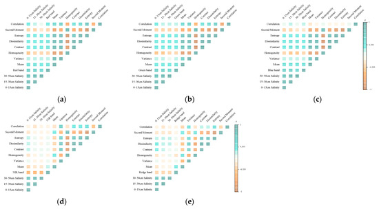
Figure 4.
Correlation between measured values of soil salinity at different depths and texture features of each spectral band. Note: (a–e) shows the correlation heat maps between the measured values of soil salinity at different depths and the texture features of red, green, blue, near-infrared and red-edge bands, respectively.
Non-linear index (NLI) and ratio vegetation index (RVI) are significantly correlated with soil salt content under alfalfa cover (Table 2). This study constructs non-linear texture indexes (NTI) and ratio texture indexes (RTI) based on the idea of vegetation index. The influence of the texture index on the accuracy of the soil salinity inversion model at different depths is also examined. The texture index is constructed by randomly selecting two of the 16 texture features in the red and blue bands, resulting in a total of 240 indexes calculated using MATLAB R2017b. The texture index calculation formulas are as follows:
NTI = (T12 − T2)/(T12 + T2)
RTI = T1/T2
In the formula, T1 and T2 represent the texture features of UAV multispectral red and blue bands.
2.5. Model Construction and Accuracy Evaluation
The salt inversion model was constructed using the RF and ELM machine learning algorithms. The modeling set consisted of 70% soil samples, and the remaining 30% was designed as the prediction set. The accuracy of the model was assessed for both the modeling set and the prediction set using several metrics, including the determination coefficient R2, the root-mean-square error (RMSE), and the mean absolute error (MAE). The closer R2 value is to 1, and the closer RMSE value is to 0, the higher the accuracy of the model. The MAE value evaluates the prediction accuracy of the model, with a smaller MAE value indicating a higher prediction accuracy. The calculation formulas are as follows:
is used for the measured soil salt content, %; to predict soil salt content, %; the average soil salt content, %; and n is the number of samples.
3. Results
3.1. Soil Salt Content Statistics
Saline–alkali soils were sampled from 62 sampling points in the alfalfa plot, including depths of 0–15 cm, 15–30 cm, and 30–50 cm. These samples were subjected to salinity statistics, and the results are depicted in Figure 5. The soil salt content decreased from one soil layer to the next, with mean values of 0.267%, 0.245%, and 0.234%, for 0–15 cm, 15–30 cm, and 30–50 cm depths, respectively. This phenomenon is due to the accumulation of salt in the lower layer of the soil that moves to the surface layer via capillary water. Soil salt content was categorized as heavy-saline–alkali soil (0.5–1%), moderately saline–alkali soil (0.2–0.5%), and light-saline–alkali soil (<0.2%), with corresponding statistics provided in Table 4. The table reveals a low degree of variation among collected soil samples, with mostly moderately saline–alkali soil. The survey results revealed that the degree of salinization in the alfalfa plot is lower than that of other vegetation-covered soils, with average soil salinity of 0.549% and 0.391% for corn and wheat, respectively [17,38]. This difference is largely attributed to the excellent saline–alkali tolerance of alfalfa, as documented in various studies where alfalfa has been shown to absorb soil salinity during growth [39,40,41].
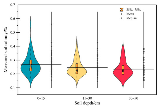
Figure 5.
Statistics of salinity at different depths.
Table 4.
Statistics of soil salinity in field sampling.
3.2. Based on the Spectral Index Inversion Model
3.2.1. Salinity Index (SIs) Construction Model
SIs were screened using grey correlation analysis. An inversion model for soil salinity at varying depths was developed using RF and ELM algorithms. The findings of the study are presented in Table 5. The RF model demonstrated an R2 value of 0.59–0.64, an RMSE of 0.029–0.039, and an MAE of 0.025–0.029, while the ELM model reflected an R2 value of 0.47–0.56, an RMSE of 0.030–0.035, and an MAE of 0.025–0.028. Overall, the RF model showed greater inversion accuracy than the ELM model. Moreover, both RF and ELM models exhibited the best inversion effect on soil salinity within depths of 0–15 cm, with R2 of 0.64 and 0.56, respectively, and small RMSE and MAE values.
Table 5.
Soil inversion models at different depths, based on SIs.
3.2.2. Vegetation Index (VIs) Construction Model
The top five most highly correlated VIs were selected to construct the inversion model. The resulting model performance metrics are presented in Table 6. The RF model achieved an R2 of 0.63–0.68, an RMSE of 0.026–0.034, and an MAE of 0.022–0.025. On the other hand, the ELM model achieved an R2 of 0.55–0.64, an RMSE of 0.028–0.039, and an MAE of 0.024–0.028. The accuracy of the RF inversion model was higher than that of the ELM model. Additionally, compared to a model constructed using SIs, the inversion model constructed with VIs as the input group exhibited significantly improved accuracy. Moreover, the inversion effect of the 0–15 cm soil layer remains the best.
Table 6.
Soil inversion models at different depths, based on VIs.
3.2.3. Salinity Index + Vegetation Index (SIs + VIs) Construction Model
To ensure the inversion accuracy of the model is not affected by too many input factors, the SIs and VIs correlation degrees in Table 2 were analyzed, and the first three indexes were selected to create the SIs + VIs input group. The accuracy evaluation of the model input and the construction of the inversion model is given in Table 7. The RF model R2 of the SIs + VIs construction model ranges from 0.58 to 0.66, while its RMSE lies within 0.028–0.034 and MAE within 0.023–0.027. The ELM model R2 ranges from 0.49 to 0.62, with RMSE and MAE ranging from 0.034–0.038 and 0.027–0.030, respectively. Although the inversion accuracy of both RF and ELM is lower than that of the VIs input model, it is higher than that of the SIs input model.
Table 7.
Soil inversion models at different depths, based on SIs + VIs.
3.3. Inversion Model Based on the Spectral Index and Texture Information
3.3.1. Vegetation Index + Texture Feature (VIs + TFs) Construction Model
Comparing Table 5, Table 6 and Table 7, it has been concluded that the inversion model constructed using VIs is superior to the models based on SIs and their combinations. The red and blue bands exhibit a significant response to soil salinity. Among the 16 texture features, the grey correlation degree between R-Cor, B-Cor, B-Ent, and the measured salt content is above 0.92, making them the top three features for each soil layer, as shown in Figure 6. The combination of VIs + TFs, including R-Cor, B-Cor, B-Ent, and VIs, is used as input to explore the effectiveness of UAV multispectral texture features in soil salinity inversion at different depths.
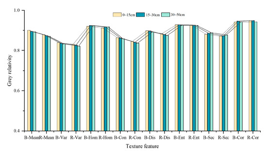
Figure 6.
Grey correlation degree of texture features.
Table 8 indicates that the RF model R2 ranges from 0.64 to 0.70, the RMSE ranges from 0.025 to 0.034, and the MAE ranges from 0.022–0.026. The ELM model R2 has an 0.62 to 0.67, an RMSE of 0.030–0.045, and an MAE of 0.023–0.034. In terms of inversion accuracy, the RF model performs better than ELM in the 0–15 cm and 30–50 cm soil layers, whereas the ELM model outperforms RF in the 15–30 cm layer. Overall, the model constructed by the VIs + TFs combination yields higher inversion accuracy than the model using VIs alone. The R2 of the RF model increases by 2.0%, the R2 of the ELM model increases by 11.1%, and the best inversion effect occurs in the 0–15 cm soil layer.
Table 8.
Soil inversion models at different depths, based on VIs + TFs.
3.3.2. Vegetation Index + Texture Index (VIs + TIs) Construction Model
The influence of texture index on the accuracy of the soil salt content inversion model at different depths was examined by constructing 480 RTIs and NTIs using 16 texture features from red and blue bands. The two types of texture indexes were sorted using grey correlation analysis, and the top three TIs and VIs were selected to construct the model (Table 9). The results showed that the VIs + TIs combination model produced a better inversion model than other input groups, and was the best performer. The RF model R2 ranged from 0.67 to 0.75, and the RMSE was between 0.023 and 0.034, whereas the MAE ranged from 0.019 to 0.026. The ELM model R2 was between 0.65 and 0.69, with the RMSE ranging from 0.027 to 0.045, and the MAE between 0.022 and 0.039. Compared to the VIs construction model, the RF model R2 and ELM model R2 increased by 8.5% and 15.8%, respectively, and the best inversion effect was observed in the 0–15 cm soil layer.
Table 9.
Soil inversion models at different depths, based on VIs + TIs.
3.4. Comprehensive Analysis
In order to explore the best inversion model and depth for soil salinity under alfalfa at varying depths, we conducted a comprehensive analysis of the inversion results of five inputs. Figure 7 presents the inversion accuracy evaluation of each model, while Figure 8 illustrates the comparison between the inversion results and the measured soil salinity. In terms of the input group, the VIs + TIs construction model showed higher R2 values compared to other input groups in the inversion study in the 0–15 cm, 15–30 cm, and 30–50 cm layers. The average R2 for the three depths in the RF model was 0.72, while the average R2 for the ELM model was 0.68. The RMSE and MAE were small, indicating better inversion results, with VIs + TFs, VIs, SIs + VIs, and SIs construction models following a descending order. Combining spectral index and texture information significantly improved the accuracy of the inversion model.
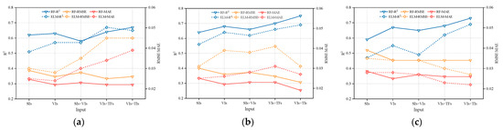
Figure 7.
Accuracy evaluation of each inversion model. (a) 0–15 cm. (b) 15–30 cm. (c) 30–50 cm.
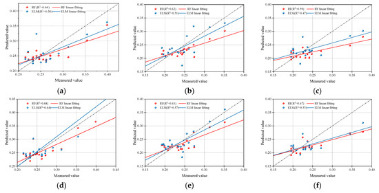
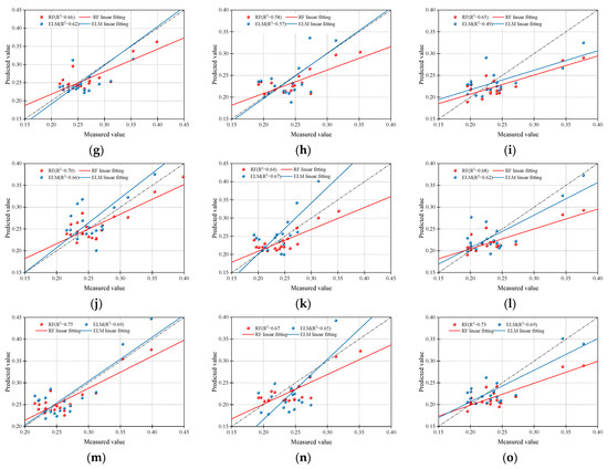
Figure 8.
Comparison of measured and predicted values of each model. (a) 0–15 cm (SIs). (b) 15–30 cm (SIs). (c) 30–50 cm (SIs). (d) 0–15 cm (VIs). (e) 15–30 cm (VIs). (f) 30–50 cm (VIs). (g) 0–15 cm (SIs + VIs). (h) 15–30 cm (SIs + VIs). (i) 30–50 cm (SIs + VIs). (j) 0–15 cm (VIs + TFs). (k) 15–30 cm (VIs + TFs). (l) 30–50 cm (VIs + TFs). (m) 0–15 cm (VIs + TIs). (n) 15–30 cm (VIs + TIs). (o) 30–50 cm (VIs + TIs).
From the perspective of the model algorithm, the RF construction model performed better than ELM. Figure 7 shows that, except for VIs + TFs in the 15–30 cm layer, the R2 of RF was higher than that of ELM. The R2 of the RF construction model ranged from 0.59–0.75, RMSE from 0.023–0.39, and MAE from 0.019–0.029. On the other hand, the R2 for the ELM construction model was 0.47–0.69, RMSE was 0.027–0.045, and MAE was 0.022–0.039. The RF model had higher inversion accuracy and better stability than ELM, with an average R2 10% higher than ELM.
From the perspective of inversion depth, it was observed that the inversion results of the RF and ELM algorithms varied. For RF, the inversion results of the 0–15 cm soil depth are better than 30–50 cm, and 15–30 cm is the worst, while for ELM, the inversion results of 0–15 cm soil depth are better than 15–30 cm, and 30–50 cm is the worst. The overall inversion effect of 0–15 cm soil salinity was found to be better, as compared to other depths. The average R2 for the five types of models constructed by RF was 0.69, with an RMSE of 0.027 and MAE of 0.022, while the average R2 for the ELM model was 0.63, with an RMSE of 0.036 and MAE of 0.027.
4. Discussion
Remote sensing images rely on image texture to convey important information. The spectral reflectance of a crop canopy has shown sensitivity towards soil salt content. Vegetation index, salt index, and texture information can be used to establish a correlation with soil salt content measured at varying depths, so as to realize multi-depth soil salt inversion [38]. To accomplish this, the research focuses on the soil at different depths under alfalfa coverage and employs various input groups, including salinity index (SIs), vegetation index (VIs), salinity index + vegetation index (SIs + VIs), vegetation index + texture feature (VIs + TFs), and vegetation index + texture index (VIs + TIs), to construct a machine learning inversion model based on RE and ELM.
When the spectral index was used to invert the soil salinity, it was observed that VIs had higher inversion accuracy than SIs and SIs + VIs modeling. This was due to the high coverage of alfalfa, making VIs sensitive to vegetation growth [42]. Zhang [18] explored the impact of different vegetation coverage on the accuracy of the soil salt content inversion model and found that the VIs construction model was more accurate under high vegetation coverage. Therefore, the model constructed by VIs can better invert soil salt content under high vegetation coverage. Based on the VIs array with a better modeling effect, the combination input of VIs + TFs and VIs + TIs was established. After analysis, the texture information of a multispectral image, combined with Vis, significantly improved the accuracy of soil salinity inversion models at different depths under vegetation cover. Compared with VIs modeling alone, the VIs + TFs construction model improved the RF model R2 by 2.0%, and the ELM model R2 by 11.1%, while the VIs + TIs combination construction model improved the RF model R2 by 8.5%, and the ELM model R2 by 15.8%. Hang [43] estimated the rice leaf area index (LAI) by combining UAV spectrum, texture features, and coverage. The multiple stepwise regression model established by combining VIs and TIs (R2 = 0.668, RMSE = 0.421) was significantly better than the single VIs model (R2 = 0.563, RMSE = 0.541). Zheng [19] also drew similar conclusions in estimating aboveground rice biomass, based on UAV image texture and spectral analysis. The integrated texture and spectral information modeling significantly improved the accuracy of rice biomass estimation. The texture features of the UAV multispectral image provide extensive information [44], making it feasible to apply to soil salinity at different depths, significantly improving the model inversion effect.
Soil models have varying accuracy levels in terms of inversion across different depths. The accuracy of the RF model for inversion in the 0–15 cm is higher than that in 30–50 cm, while the performance in the 15–30 cm is poor. However, for the ELM model, the inversion results in 0–15 cm are better than those in 15–30 cm, while the performance for 30–50 cm is worst. Overall, the inversion effect of soil salinity is best in 0–15 cm. The RF model has an average R2 of 0.69, RMSE of 0.027, and MAE of 0.022, whereas the ELM model has an average R2 of 0.63, RMSE of 0.036, and MAE of 0.027. Wang [9] drew a similar conclusion in the inversion of soil salinity in the Kuqa Oasis. The highest accuracy was observed in the 0–10 cm model, with an R2 between 0.60 and 0.74. Yang [26] also showed that the 0–20 cm layer contained the main root system of the crop, and the UAV could capture surface soil spectral information directly. The correlation between soil salinity and various types of spectral and texture information gradually decreased with depth.
In this study, the overall performance of the model based on the RF algorithm was better than that of ELM. The R2 of the RF model ranged from 0.59 to 0.75, RMSE ranged from 0.023 to 0.39, and MAE ranged from 0.019 to 0.029. The R2 of the ELM model ranged from 0.47 to 0.69, RMSE ranged from 0.027 to 0.045, and the MAE ranged from 0.022 to 0.039. Many scholars have compared the inversion models of related soil parameters and concluded that the RF model has greater applicability and stability, and its performance ability is more prominent than other algorithms [45,46]. Therefore, it can be used for accurate modeling of soil salt inversion.
5. Conclusions
The research conclusions are summarized as follows:
- (1)
- The VIs construction model showed better inversion accuracy than the SIs and SIs + VIs models in the spectral index modeling.
- (2)
- The combination of texture information with VIs improved the inversion accuracy. The VIs + TIs model showed the best inversion effect, and the second-best model was the VIs + TFs. Compared to the VIs modeling, the RF model R2 of VIs + TIs and VIs + TFs increased by 8.5% and 2.0%, and the ELM model R2 increased by 15.8% and 11.1%, respectively.
- (3)
- The inversion effect of 0–15 cm soil salinity was significantly better than that of other depths, and was the best inversion depth of soil salinity under alfalfa cover. The average R2 for the five types of models constructed by RF was 0.69, while the average R2 for the ELM model was 0.63.
- (4)
- The RF model performed better than the ELM in soil salinity inversion. The RF average R2 was 10% higher than the ELM. The R2 of the RF model ranged from 0.59–0.75, while the R2 for the ELM construction model was 0.47–0.69.
The findings of our study will primarily be applied to small-scale soil salinity research in alfalfa fields with conditions similar to those in northwest China. These results will contribute to formulating strategies for managing soil salinization and crop growth. Future research will involve extrapolating these findings to larger areas and other crop-growing regions, or corroborating the universality of multispectral texture information in soil salinity inversion through conjunction with satellite datasets, to subsequently enhance the accuracy and robustness of soil salinity inversion models under crop cover.
Author Contributions
Formal analysis, F.M.; funding acquisition, W.Z. and F.M.; methodology, F.M. and W.Z.; project administration, W.Z. and H.Y.; software, Z.L. and F.M.; validation, Z.L.; writing—original draft, F.M.; writing—review and editing, F.M. and H.Y. All authors have read and agreed to the published version of the manuscript.
Funding
This research was funded by the National Natural Science Foundation of China (51869010).
Institutional Review Board Statement
Not applicable.
Data Availability Statement
Data not available due to commercial restrictions.
Conflicts of Interest
The authors declare no conflict of interest.
References
- Aldabaa, A.; Weindorf, D.C.; Chakraborty, S.; Sharma, A.; Li, B. Combination of proximal and remote sensing methods for rapid soil salinity quantification. Geoderma 2015, 239, 34–46. [Google Scholar] [CrossRef]
- Hassani, A.; Azapagic, A.; Shokri, N. Global predictions of primary soil salinization under changing climate in the 21st century. Nat. Commun. 2021, 12, 6663. [Google Scholar] [CrossRef]
- Allbed, A.; Kumar, L.; Aldakheel, Y.Y. Assessing soil salinity using soil salinity and vegetation indices derived from IKONOS high-spatial resolution imageries: Applications in a date palm dominated region. Geoderma 2014, 230, 1–8. [Google Scholar] [CrossRef]
- Ding, J.; Yu, D. Monitoring and evaluating spatial variability of soil salinity in dry and wet seasons in the Werigan–Kuqa Oasis, China, using remote sensing and electromagnetic induction instruments. Geoderma 2014, 235, 316–322. [Google Scholar] [CrossRef]
- Chen, J.; Yao, Z.; Zhang, Z.; Wei, G.; Wang, X.; Han, J. UAV Remote Sensing Inversion of Soil Salinity in Field of Sunflower. Trans. Chin. Soc. Agric. Mach. 2020, 51, 178–191. [Google Scholar] [CrossRef]
- Weng, Y.-L.; Gong, P.; Zhu, Z.-L. A Spectral Index for Estimating Soil Salinity in the Yellow River Delta Region of China Using EO-1 Hyperion Data. Pedosphere 2010, 20, 378–388. [Google Scholar] [CrossRef]
- Hu, J.; Peng, J.; Zhou, Y.; Xu, D.; Zhao, R.; Jiang, Q.; Fu, T.; Wang, F.; Shi, Z. Quantitative Estimation of Soil Salinity Using UAV-Borne Hyperspectral and Satellite Multispectral Images. Remote Sens. 2019, 11, 736. [Google Scholar] [CrossRef]
- Zhang, T.-T.; Qi, J.-G.; Gao, Y.; Ouyang, Z.-T.; Zeng, S.-L.; Zhao, B. Detecting soil salinity with MODIS time series VI data. Ecol. Indic. 2015, 52, 480–489. [Google Scholar] [CrossRef]
- Wang, F.; Shi, Z.; Biswas, A.; Yang, S.; Ding, J. Multi-algorithm comparison for predicting soil salinity. Geoderma 2020, 365, 114211. [Google Scholar] [CrossRef]
- Abuzaid, A.S.; El-Komy, M.S.; Shokr, M.S.; El Baroudy, A.A.; Mohamed, E.S.; Rebouh, N.Y.; Abdel-Hai, M.S. Predicting Dynamics of Soil Salinity and Sodicity Using Remote Sensing Techniques: A Landscape-Scale Assessment in the Northeastern Egypt. Sustainability 2023, 15, 9440. [Google Scholar] [CrossRef]
- Niu, B.; Li, X.; Li, F.; Wang, Y.; Hu, X. Vegetation dynamics and its linkage with climatic and anthropogenic factors in the Dawen River Watershed of China from 1999 through. Environ. Sci. Pollut. Res. 2021, 28, 52887–52900. [Google Scholar] [CrossRef]
- Zhang, Z.; Niu, B.; Li, X.; Kang, X.; Wan, H.; Shi, X.; Li, Q.; Xue, Y.; Hu, X. Inversion of soil salinity in China’s Yellow River Delta using unmanned aerial vehicle multispectral technique. Environ. Monit. Assess. 2023, 195, 245. [Google Scholar] [CrossRef]
- Romero-Trigueros, C.; Nortes, P.A.; Alarcón, J.J.; Hunink, J.E.; Parra, M.; Contreras, S.; Droogers, P.; Nicolás, E. Effects of saline reclaimed waters and deficit irrigation on Citrus physiology assessed by UAV remote sensing. Agric. Water Manag. 2017, 183, 60–69. [Google Scholar] [CrossRef]
- Yu, J.; Wang, J.; Leblon, B. Evaluation of Soil Properties, Topographic Metrics, Plant Height, and Unmanned Aerial Vehicle Multispectral Imagery Using Machine Learning Methods to Estimate Canopy Nitrogen Weight in Corn. Remote Sens. 2021, 13, 3105. [Google Scholar] [CrossRef]
- Ge, X.; Ding, J.; Jin, X.; Wang, J.; Chen, X.; Li, X.; Liu, J.; Xie, B. Estimating Agricultural Soil Moisture Content through UAV-Based Hyperspectral Images in the Arid Region. Remote Sens. 2021, 13, 1562. [Google Scholar] [CrossRef]
- Zhu, C.; Ding, J.; Zhang, Z.; Wang, Z. Exploring the potential of UAV hyperspectral image for estimating soil salinity: Effects of optimal band combination algorithm and random forest. Spectrochim. Acta Part A Mol. Biomol. Spectrosc. 2022, 279, 121416. [Google Scholar] [CrossRef]
- Zhao, W.; Zhou, C.; Zhou, C.; Ma, H.; Wang, Z. Soil Salinity Inversion Model of Oasis in Arid Area Based on UAV Multispectral Remote Sensing. Remote Sens. 2022, 14, 1804. [Google Scholar] [CrossRef]
- Zhang, Z.; Tai, X.; Yang, N.; Zhang, J.; Huang, X.; Chen, Q. Inversion of soil salt content by UAV remote sensing under different vegetation coverage. Trans. Chin. Soc. Agric. Mach. 2022, 53, 220–230. [Google Scholar]
- Zheng, H.; Ma, J.; Zhou, M.; Li, D.; Yao, X.; Cao, W.; Zhu, Y.; Cheng, T. Enhancing the Nitrogen Signals of Rice Canopies across Critical Growth Stages through the Integration of Textural and Spectral Information from Unmanned Aerial Vehicle (UAV) Multispectral Imagery. Remote Sens. 2020, 12, 957. [Google Scholar] [CrossRef]
- Zhang, J.; Cheng, T.; Shi, L.; Wang, W.; Niu, Z.; Guo, W.; Ma, X. Combining spectral and texture features of UAV hyperspectral images for leaf nitrogen content monitoring in winter wheat. Int. J. Remote Sens. 2022, 43, 2335–2356. [Google Scholar] [CrossRef]
- Cheng, M.; Jiao, X.; Liu, Y.; Shao, M.; Yu, X.; Bai, Y.; Wang, Z.; Wang, S.; Tuohuti, N.; Liu, S.; et al. Estimation of soil moisture content under high maize canopy coverage from UAV multimodal data and machine learning. Agric. Water Manag. 2022, 264, 107530. [Google Scholar] [CrossRef]
- Sun, Q.; Sun, L.; Shu, M.; Gu, X.; Yang, G.; Zhou, L. Monitoring Maize Lodging Grades via Unmanned Aerial Vehicle Multispectral Image. Plant Phenomics 2019, 2019, 5704154. [Google Scholar] [CrossRef]
- Zheng, H.B.; Cheng, T.; Zhou, M.; Li, D.; Yao, X.; Tian, Y.C.; Cao, W.X.; Zhu, Y. Improved estimation of rice aboveground biomass combining textural and spectral analysis of UAV imagery. Precis. Agric. 2019, 20, 611–629. [Google Scholar] [CrossRef]
- Wei, G.; Li, Y.; Zhang, Z.; Chen, Y.; Chen, J.; Yao, Z.; Lao, C.; Chen, H. Estimation of soil salt content by combining UAV-borne multispectral sensor and machine learning algorithms. PeerJ 2020, 8, e9087. [Google Scholar] [CrossRef]
- Wang, Z.; Zhang, F.; Zhang, X.; Chan, N.W.; Kung, H.-T.; Ariken, M.; Zhou, X.; Wang, Y. Regional suitability prediction of soil salinization based on remote-sensing derivatives and optimal spectral index. Sci. Total Environ. 2021, 775, 145807. [Google Scholar] [CrossRef]
- Yang, N.; Cui, W.; Zhang, Z.; Zhang, J.; Chen, J.; Du, R.; Lao, C.; Zhou, Y. Inversion of soil salinity at different depths by UAV multispectral remote sensing. Trans. Chin. Soc. Agric. Eng. 2020, 36, 13–21. [Google Scholar] [CrossRef]
- Zhang, F.; Tashpolat, T.; Ding, J.; Tian, Y.; Mamat, S. Relationships between soil salinization and spectra in the delta oasis of Weigan and Kuqa Rivers. Res. Environ. Sci. 2009, 22, 227–235. [Google Scholar]
- Huang, Q.; Xu, X.; Lü, L.; Ren, D.; Ke, J.; Xiong, Y.; Huo, Z.; Huang, G. Soil salinity distribution based on remote sensing and its effect on crop growth in Hetao Irrigation District. Trans. Chin. Soc. Agric. Eng. 2018, 34, 102–109. [Google Scholar] [CrossRef]
- Zhang, Z.; Tan, C.; Xu, C.; Chen, S.; Han, W.; Li, Y. Retrieving Soil Moisture Content in Field Maize Root Zone Based on UAV Multispectral Remote Sensing. Trans. Chin. Soc. Agric. Mach. 2019, 50, 246–257. [Google Scholar] [CrossRef]
- Chang, A.; Yeom, J.; Jung, J.; Landivar, J. Comparison of Canopy Shape and Vegetation Indices of Citrus Trees Derived from UAV Multispectral Images for Characterization of Citrus Greening Disease. Remote Sens. 2020, 12, 4122. [Google Scholar] [CrossRef]
- Kaplan, G.; Avdan, U. Evaluating the utilization of the red edge and radar bands from sentinel sensors for wetland classification. Catena 2019, 178, 109–119. [Google Scholar] [CrossRef]
- Wang, J.; Ding, J.; Yu, D.; Ma, X.; Zhang, Z.; Ge, X.; Teng, D.; Li, X.; Liang, J.; Lizaga, I.; et al. Capability of Sentinel-2 MSI data for monitoring and mapping of soil salinity in dry and wet seasons in the Ebinur Lake region, Xinjiang, China. Geoderma 2019, 353, 172–187. [Google Scholar] [CrossRef]
- Zheng, Q.; Huang, W.; Cui, X.; Shi, Y.; Liu, L. New Spectral Index for Detecting Wheat Yellow Rust Using Sentinel-2 Multispectral Imagery. Sensors 2018, 18, 868. [Google Scholar] [CrossRef] [PubMed]
- Guo, Y.; Zhang, X.; Chen, S.; Wang, H.; Jayavelu, S.; Cammarano, D.; Fu, Y. Integrated UAV-Based Multi-Source Data for Predicting Maize Grain Yield Using Machine Learning Approaches. Remote Sens. 2022, 14, 6290. [Google Scholar] [CrossRef]
- Guo, Y.; Chen, S.; Wu, Z.; Wang, S.; Bryant, C.R.; Senthilnath, J.; Cunha, M.; Fu, Y.H. Integrating Spectral and Textural Information for Monitoring the Growth of Pear Trees Using Optical Images from the UAV Platform. Remote Sens. 2021, 13, 1795. [Google Scholar] [CrossRef]
- Wang, L.; He, J.; Zheng, G.; Guo, Y.; Zhang, Y.; Zhang, H. Estimation of Maize FPAR Based on UAV Multispectral Remote Sensing. Trans. Chin. Soc. Agric. Mach. 2022, 53, 202–210. [Google Scholar] [CrossRef]
- Xiao, Y.; Dong, Y.; Huang, W.; Liu, L.; Ma, H. Wheat Fusarium Head Blight Detection Using UAV-Based Spectral and Texture Features in Optimal Window Size. Remote Sens. 2021, 13, 2437. [Google Scholar] [CrossRef]
- Zhao, W.; Ma, F.; Ma, H.; Zhou, C. Soil salinity inversion model based on multispectral image of UAV. Trans. Chin. Soc. Agric. Eng. 2022, 38, 93–101. [Google Scholar] [CrossRef]
- Shah, S.H.H.; Wang, J.; Hao, X.; Thomas, B.W. Modelling soil salinity effects on salt water uptake and crop growth using a modified denitrification-decomposition model: A phytoremediation approach. J. Environ. Manag. 2022, 301, 113820. [Google Scholar] [CrossRef]
- Lu, Q.; Ge, G.; Sa, D.; Wang, Z.; Hou, M.; Jia, Y.S. Effects of salt stress levels on nutritional quality and microorganisms of alfalfa-influenced soil. PeerJ 2021, 9, e11729. [Google Scholar] [CrossRef]
- Qiu, Y.; Wang, Y.; Fan, Y.; Hao, X.; Li, S.; Kang, S. Root, Yield, and Quality of Alfalfa Affected by Soil Salinity in Northwest China. Agriculture 2023, 13, 750. [Google Scholar] [CrossRef]
- Zhang, Z.; Wei, G.; Yao, Z.; Tan, C.; Wang, X.; Han, J. Soil salt inversion model based on UAV multispectral remote sensing. Trans. Chin. Soc. Agric. Mach. 2019, 50, 151–160. [Google Scholar] [CrossRef]
- Hang, Y.; Su, H.; Yu, Z.; Liu, H.; Guan, H.; Kong, F. Estimation of rice leaf area index combining UAV spectrum, texture features and vegetation coverage. Trans. Chin. Soc. Agric. Eng. 2021, 37, 64–71. [Google Scholar] [CrossRef]
- Guo, Y.; Fu, Y.H.; Chen, S.; Bryant, C.R.; Li, X.; Senthilnath, J.; Sun, H.; Wang, S.; Wu, Z.; de Beurs, K. Integrating spectral and textural information for identifying the tasseling date of summer maize using UAV based RGB images. Int. J. Appl. Earth Obs. Geoinformation 2021, 102, 102435. [Google Scholar] [CrossRef]
- Ge, X.; Wang, J.; Ding, J.; Cao, X.; Zhang, Z.; Liu, J.; Li, X. Combining UAV-based hyperspectral imagery and machine learning algorithms for soil moisture content monitoring. PeerJ 2019, 7, e6926. [Google Scholar] [CrossRef]
- Lindner, C.; Bromiley, P.A.; Ionita, M.C.; Cootes, T.F. Robust and Accurate Shape Model Matching Using Random Forest Regression-Voting. IEEE Trans. Pattern Anal. Mach. Intell. 2014, 37, 1862–1874. [Google Scholar] [CrossRef]


Disclaimer/Publisher’s Note: The statements, opinions and data contained in all publications are solely those of the individual author(s) and contributor(s) and not of MDPI and/or the editor(s). MDPI and/or the editor(s) disclaim responsibility for any injury to people or property resulting from any ideas, methods, instructions or products referred to in the content. |
© 2023 by the authors. Licensee MDPI, Basel, Switzerland. This article is an open access article distributed under the terms and conditions of the Creative Commons Attribution (CC BY) license (https://creativecommons.org/licenses/by/4.0/).