Article

Lettuce Plant Trace-Element-Deficiency Symptom Identification via Machine Vision Methods

1
Modern Agricultural Equipment Research Institute, School of Mechanical Engineering, Xihua University, Chengdu 610039, China
2
School of Mechanical Engineering, Xihua University, Chengdu 610039, China
3
Chengdu Academy of Agriculture and Foresty Science, Chengdu 611130, China
*
Author to whom correspondence should be addressed.
Agriculture 2023, 13(8), 1614; https://doi.org/10.3390/agriculture13081614
Submission received: 12 July 2023 / Revised: 7 August 2023 / Accepted: 10 August 2023 / Published: 15 August 2023

Abstract

:
Lettuce is one of the most widely planted leafy vegetables in plant factories. The lack of trace elements in nutrient solutions has caused huge losses to the lettuce industry. Non-obvious symptoms of trace element deficiency, the inconsistent size of the characteristic areas, and the difficulty of extraction in different growth stages are three key problems affecting lettuce deficiency symptom identification. In this study, a batch of cream lettuce (lactuca sativa) was planted in the plant factory, and its nutrient elements were artificially controlled. We collected images of the lettuce at different growth stages, including all nutrient elements and three nutrient-deficient groups (potassium deficiency, calcium deficiency, and magnesium deficiency), and performed feature extraction analysis on images of different defects. We used traditional algorithms (k-nearest neighbor, support vector machine, random forest) and lightweight deep-learning models (ShuffleNet, SqueezeNet, andMobileNetV2) for classification, and we compared different feature extraction methods (texture features, color features, scale-invariant feature transform features). The experiment shows that, under the optimal feature extraction method (color), the random-forest recognition results are the best, with an accuracy rate of 97.6%, a precision rate of 97.9%, a recall rate of 97.4%, and an F1 score of 97.6%. The accuracies of all three deep-learning models exceed 99.5%, among which ShuffleNet is the best, with the accuracy, precision, recall, and F1 score above 99.8%. It also uses fewer floating-point operations per second and less time. The proposed method can quickly identify the trace elements lacking in lettuce, and it can provide technical support for the visual recognition of the disease patrol robot in the plant factory.

1. Introduction

In labor work, people usually focus on the use of large amounts of elements, like N, P, and K, while they ignore the supply of trace elements, including Ca, Mg, and Fe. This unreasonable fertilization by humans, as well as differences in the nutrient statuses of different regions or types of soils, lead to the widespread occurrence of plant physiological diseases [1]. Compared with plant pathological diseases, plant physiological diseases are not infectious. However, they affect the plant cultivation area, leaf color, number of leaves, and plant height, which cause significant decreases in agricultural yields. Therefore, the efficient and accurate identification of plant physiological diseases is particularly important.
At present, there are manual methods, morphological methods, and chemical methods for plant disease identification. The manual diagnosis method is subjective and requires excellent expertise, especially in the early growth stage [2,3]. With the morphological method, symptoms of plant diseases can be visualized from morphological characteristics (such as leaf color, leaf shape, etc.) so that the lacking nutrients can be correctly identified. When the lack of symptoms are visible, the reduction in the yield may have already occurred [4]. Chemical methods have high accuracy and stability, but they are time-consuming and costly, making them unsuitable for promotion in agricultural production [5]. With the development of agricultural information and artificial intelligence and the rise of machine learning, plant disease detection and classification have new research ideas.
Machine-learning techniques have yielded good results in many fields [6,7,8,9]. Because leaves are the main expression of plant diseases, the analysis of crop images using computer vision methods can detect diseases earlier than human-eye observation [10]. Industrial cameras, hyperspectral cameras, mobile phones, and other devices are used to collect plant leaf images to determine the health of the leaves, and then the sensor sends the results to the control center in real time for the automatic identification of plant diseases, as well as by the mobile side to take images back to the server for disease identification, thus improving the production efficiency over the manual method. The excessive use of pesticides can have a negative impact on the environment. Govardhan M et al. [11] argued that distinguishing the detection of diseases from nutritional deficiencies has a very significant impact on determining the need for pesticides. Balakrishna K et al. [12] presented a comprehensive study of the KNN (k-nearest neighbor) and PNN (probabilistic neural network) for the detection and classification of tomato leaf diseases, with a classification performance of 91.88%. Paul et al. [13] proposed a lightweight, custom convolutional neural network (CNN) model, and used the transfer learning (TL)-based models VGG-16 and VGG-19 to classify 11 categories of tomato leaf diseases. Through the application of data enhancement technology, the proposed model reached the highest accuracy and recall rate of 95.00%. Qin et al. [14] collected the images of alfalfa pseudopeziza medicaginis, rust, leptosphaerulina leaf spot, and cercospora leaf spot, and identified the diseases based on a CNN and support vector machine. Syed-Ab-Rahman S F et al. [15] used a two-stage deep CNN (convolution neural network) model for plant disease detection and citrus disease classification using leaf images, the average detection accuracy of which was 95.8%. Agarwal M et al. [16] proposed a simplified CNN model consisting of eight hidden layers for the classification of nine diseases of tomato, achieving a correct rate of 98.4%. Trang K et al. [10] proposed a method to identify plant diseases via a set of acquired leaf images. Junde Chena et al. [17] used a deep convolutional neural network for the migration-learning approach in plant leaf disease identification. The validation accuracy on publicly available datasets was no less than 91.83%. Francis M et al. [18] developed a convolutional neural network model for plant disease detection and classification using PlantVillage images containing 3663 images with an 87% training accuracy. Militante SV et al. [19] used a robust model-based CNN for apple leaf disease black-rot detection. The accuracy of the trained model could reach 96.5%. Azimi S. [20] compared deep-learning techniques and found that Resnet18 and NasNet Large (with millions of trainable parameters) can obtain ceiling-level stress classification from plant seedling images.
Most studies focus on pathological diseases of single plants, but very few studies have been conducted on physiological plant diseases. Ghosal et al. [21] also used the machine-learning framework to conduct experiments on soybean leaf deficiency. Most studies are based on visual diseases. Tran et al. [22] used GBT for recognition without visual symptoms, but the accuracy was not high. Xu et al. [23] used deep convolutional networks and traditional machine-learning methods to identify rice deficiency symptoms, and the results showed that the InceptionV3 was superior to other classification models. Yi et al. [24] used five different deep-learning networks to identify symptoms of sugar beet deficiency. Their data samples were relatively small due to the limited number of disease species. Due to the special nature of plant growth, the detection accuracy will be affected by environmental conditions and nutrient supply factors [25]. Most critical environmental factor affecting lettuce growth was nutrients [26]. Lettuce, a vegetable widely grown in plant factories, has a sensitive response to light. Light intensity or weakness can seriously affect its yield and quality. These differences can be captured in images and classified using fine-grained classification methods. However, traditional fine-grained recognition techniques still face extreme challenges in dealing with the classification among such species. To address this issue, Hao X et al. [27] established a set of light-stressed graded leaf images of lettuce as a research subject. Taha M F et al. [5] aimed to combine color imaging techniques with deep convolutional neural networks (DCNNS) to diagnose nutritional status of aquaponics lettuce. Plant electrophysiological data can detect and analyze nutrient deficiencies, which can be classified using signal decomposition and two-level measurements [28]. Detecting and classifying nutrient deficiencies at an early stage way can facilitate early plant disease preventative and therapeutic approaches at the onset of symptoms and also can help to promote plant growth [29].
Most existing studies on plant disease recognition either explore only traditional machine learning algorithms or only deep learning algorithms, and relatively few studies compare the two simultaneously. Most datasets are for single plant pathological diseases, and there are few studies on plant physiological diseases. The literature on vegetation deficiency identification rarely considers inconsistent symptom sizes over growth stages, making feature extraction and distinction difficult. When using the spectral image recognition method, there is a large intra-class gap in the plant leaf spectra and a high redundancy of deficiency spectral data. It also requires expensive equipment and controlled light conditions, which have the problem of high cost. When a spectral image recognition method is used, there is a large intra-class gap in the spectra of plant leaves, the lack of spectral data has a high redundancy, and expensive equipment and controllable lighting conditions are required, which has a high cost problem. There are few applications in the field of early plant defect identification, especially for plant factories. Accurately and intelligently identifying factory plant defects has become a new research hotspot.
In this paper, traditional machine learning methods and deep learning methods were used to extract images of factory-grown lettuce lacking nutrient solution elements at different growth stages, identify the symptom of trace element deficiency and the sizes of characteristic areas, and find the optimal recognition method.

2. Materials and Methods

2.1. Deficiency Samples Preparation

The lettuce variety was cream lettuce “Butterhead”. The lettuce cultivation process includes seedling, transplanting, and hydroponics stages. Figure 1 shows the different growth stages of lettuces.
The experiment was conducted at the Chengdu Academy of Agriculture and Forestry Sciences at 30 degrees Celsius and 53% humidity. Deficient lettuces indifferent nutrient elements were controlled manually and the samples were grown in a plant factory (Figure 2).
During preparation of the lettuce deficiency samples, pure water was used to prepare the nutrient solution. With the whole growth process, no more nutrient would be added separately. The ratios of the nutrient solutions are shown in Table 1.
According to the actual production conditions in plant factories, the experimental data were divided into four categories—a control group with all nutrient elements (“CK”), and three nutrient deficient groups: calcium deficiency (“-Ca”), magnesium deficiency (“-Mg”), and potassium deficiency (“-K”).
Two batches of lettuce were cultivated between June to August 2021. Each category had 27 plants in the first experiment and 18 plants in the second experiment. The symptoms of nutrient deficiency in the lettuces are shown in Figure 3.
Calcium-deficient plants grow normally in the early stage of hydroponics, and the old leaves do not show any calcium deficiency symptoms. In the middle stage, the new young leaves exhibit a heartburn phenomenon, which leads the plants to rapid necrosis of the growth point. The potassium-deficient plants showed interveinal greenness. Compared to healthy plants, potassium-deficient plants grow more slowly and have longer, shorter leaves. The earliest signs of magnesium deficiency in magnesium deficient plants are the old leaves at the lower part of the plant starting to turn yellow from the edge of the leaf inward. Finally, all the leaves gradually turn yellow, and the whole plant grows slowly, lower than the healthy plant.
Lettuce seedlings were transplanted to colonization plates on 16 June 2021. When cultured on 5 July, the plants showed obvious deficiency symptoms. Data collection was conducted on half the plants. Among them, the lettuce with calcium deficiency already showed the heartburn deficiency characteristic at the first time. The growth point would soon die. So, we collected all the sample images of the lettuce of “-Ca”. On 19 July, we conducted the second image acquisition for the other three lettuce groups. The purpose of collecting images in two stages was to consider the changes of vegetative deficiency characteristics of lettuce plants in different physiological stages of growth and ensure the diversity of data. On 21 July, the second deficiency experiment was carried out with 18 plants per category under the same controlled conditions.

2.2. Image Collection

During the experiment, both industrial cameras and mobile cameras were used to collect image data. A Huawei Honor V30 mobile phone captured “jpg” images. An industrial camera was used with a bracket and ring light. The bracket was a 900 mm threaded rod support, the ring light was 6–10 w white band (400–1000 nm), and the industrial camera was a MER-125-30GC. The resolutions were 1640 × 3648 pixels and 3000 × 4000 pixels, respectively. The phone was 15-40 cm from the target, and the images were taken between 9:00 a.m. and 5:00 p.m.
There are very few publicly available datasets for plant deficiencies, and labeled data can greatly affect model performance for neural networks relying on labeled data. During shooting, the whole lettuce was placed on a uniform illumination background. Shooting conditions were selected to make the light evenly distributed over the whole plant. The camera lens was kept parallel to the leaf surface of the plant as far as possible to avoid obvious deformation. In total, 825 images were collected in the two experiments, including 175 for calcium deficiency, 172 for magnesium deficiency, 226 for potassium depletion, and 252 for healthy.

2.3. Image Pre-Processing

After image collection, it is necessary to manually screen the images to eliminate the blurred images and the images without foreground objects. After screening, we use the “Image Tuner” image processing tool to expand the image sample, such as rotation, mirroring, texture enhancement and other operations. In order to realize the feature extraction operation, the data samples need to be gray-scaled, channel separation, and other operations. Texture, color, and SIFT features were integrated to obtain the feature parameters of the plant disease images. The classical traditional machine learning algorithms—support vector machine (SVM), k-nearest neighbor (KNN), and random forest—were used to identify the physiological diseases of cream lettuce deficiency.
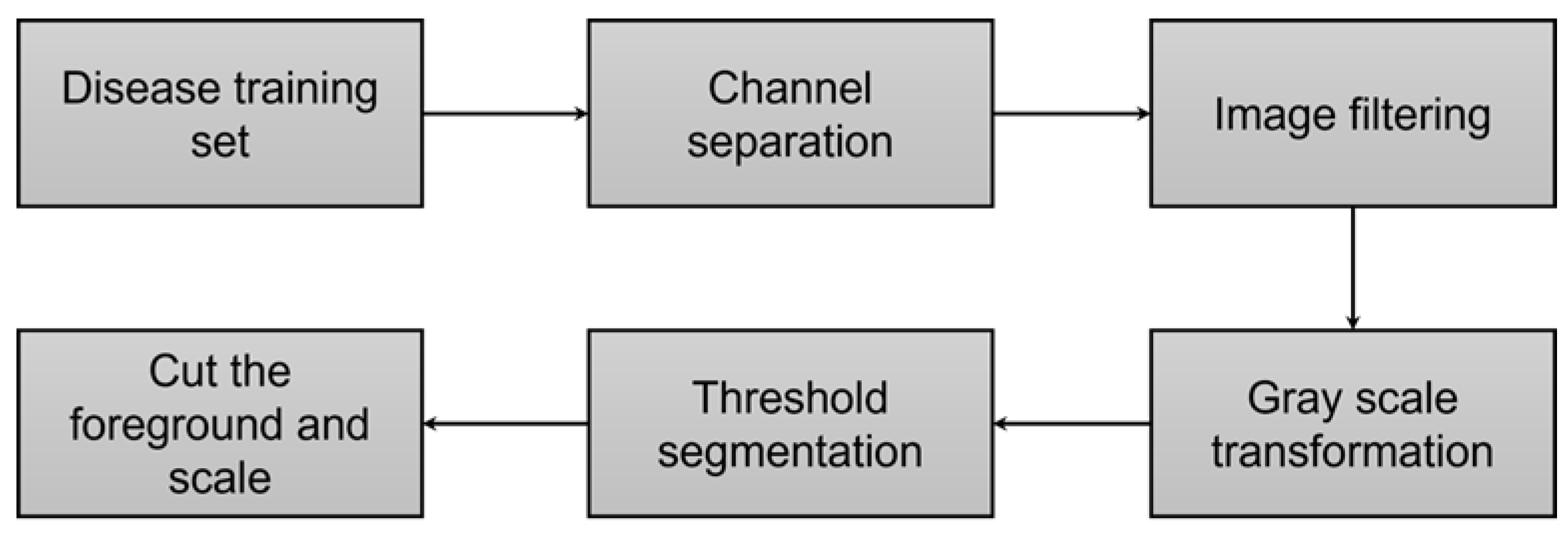
Before training the machine learning algorithms, the preprocessing of data set can improve the performance and convergence speed of the model. The lettuce image taken in the experiment had the problems of large area occupied by the background and complex background. If the background segmentation is not performed, it will not only interfere with the feature extraction of the disease image, but also produce unnecessary computation. Image pre-processing is shown in Figure 4.

2.4. Disease Image Features Extraction

Image features are acquired in traditional machine learning algorithms to classify different nutrient groups. Since plant diseases usually exhibit distinct color features [30,31] and texture features [32,33], the feature extraction stage mainly extracts these two types of features. For texture features, we used feature extraction methods include Gray Level Co-occurrence Matrix (GLCM) [34] and Local Binary Pattern (LBP). For color features, common feature extraction methods include color moments and color histograms. To better extract disease features, we also used scale-invariant feature transform (SIFT) algorithm to capture disease edge features.

2.4.1. Texture Feature

Texture features were extracted using GLCM [34] in four directions. The greyscale values were first compressed from 256 to 16 levels in order to enhance the processing speed. The notational indices, i and j are defined as the grey tone values of pixels of g u , v and g m , n where u and m are located in the x-coordinate, while v and n are located in the y-coordinate. The notational value, d is the distance between g ( u ,   v ) and g ( m ,   n ) , and h is the angle between g u , v and g m , n where h can be 0°, 45°, 90°, or 135°. The results are represented as   p   i , j , d , h , which can be further normalized using Equation (1).
P i , j , d , θ = p i , j , d , θ N
where p i , j , d , h is the normalized matrix element values and N is the summation of all the leaf pixels element values in the matrix. There were 4 parameters [35] calculated in 4 directions (0°, 45°, 90° and 135°) using Equations (2)–(5) to represent the grey distribution and texture roughness of lettuce plants.
Angular Second Moment ( A S M ):
A S M = i j P i , j , d , θ 2
Entropy ( E N T ):
E N T = i j P i , j , d , θ log P i , j , d , θ
Contrast ( C O N ):
C O N = i j i j 2 P i , j , d , θ
Correlation ( C O R ) :
C O R = i j i × j P i , j , d , θ μ x μ y σ x σ y
where:
μ x = i j i × P i , j , d , θ ,                 μ y = i j j × P i , j , d , θ
σ x = i j i μ x 2 × P i , j , d , θ , σ y = i j i μ y 2 × P i , j , d , θ  
Proposed by [36] in 1994, the local binary pattern is a special operator used to describe the local texture features of images, which has the advantages of rotation and gray invariance. The original LBP operator was defined in a 3 × 3 window, and the center pixel of the window was used as the gray threshold, and the gray value of the surrounding 8 pixels was compared with the center pixel value. If the value of the adjacent pixel exceeds the threshold, the position value of the adjacent pixel will be marked as 1, otherwise it will be marked as 0 [37,38]. From this, an 8-bit binary number can be generated and converted to a decimal number to obtain the LBP values of the center pixel, which is used as the texture feature of the reflection domain. In order to meet different application requirements, researchers have proposed a variety of improved LBP operators on the basis of the original LBP operators, such as Uniform Patterns [39], to solve the problem of too many binary patterns, and rotation invariant LBP [40].

2.4.2. Color Features

In 1995, Stricker and Orengo [41] proposed color moments, which is a simple and efficient way to describe color features. Since image color information is mostly concentrated in low-order moments, it is sufficient to describe image color distribution by using the first-order moments (Mean), second-order moments (Variance) and third-order moments (Skewness). These three parameters can be obtained by the following Equations (6)–(8).
Mean ( E i ):
E i = 1 N j = 1 N P i , j
Standard deviation ( σ i ):
σ i = 1 N j = 1 N p i , j E i 2 1 2
Skewness ( s i ):
s i = 1 N j = 1 N p i , j E i 3 1 3
where, p i and j represent the occurrence probability of pixels with gray level j in the ith color channel component of the color image, and N represents the number of pixels in the image. Michael et al. [42] first proposed color histograms, as a description method of image color features. The color histograms divides the color space evenly, calculates the percentage of each color in the pixel of the image [43], and simply describes the overall distribution of color in the image. It has the advantage of invariance to rotation and translation.

2.4.3. Scale-Invariant Feature

SIFT (scale-invariant feature transform) is a kind of operator used to describe the local features of image, which has the property of scale invariance, and when the shooting angle is changed, the same good detection effect can be obtained. The whole algorithm mainly includes the following steps: constructing the scale space, detecting key points in the scale space, locating them, and generating the feature description.
(1)
Constructing the scale space
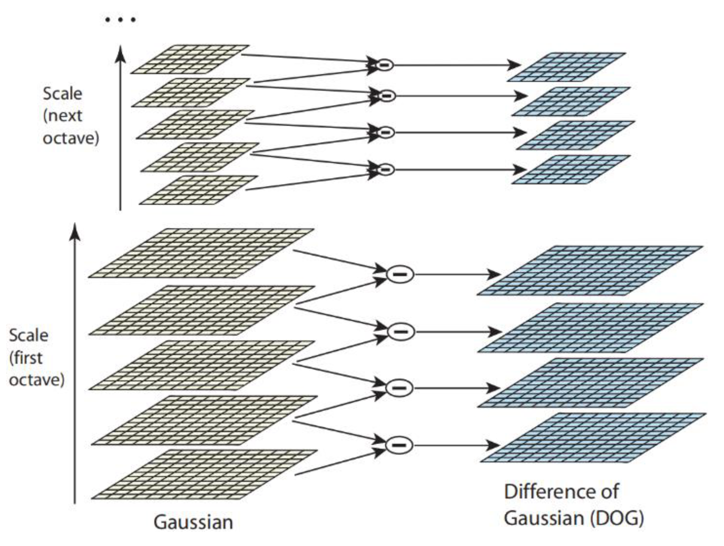
In order to achieve scale invariance of image feature points, SIFT algorithm uses Gaussian scale space to describe image scale space [44]. Firstly, Gaussian kernels of different scales (different values) are used for convolution of the original image, and then the next set of image samples are formed by taking points at different intervals (subsampling). The above operations are repeated to build the Gaussian pyramid. Then, the same group of sample pictures are differentially operated to build a Gaussian difference pyramid and form a scale space, as shown in Figure 5.
Image scale space can be expressed as Equations (9) and (10):
G x , y , σ = 1 2 π σ 2 e x 2 + y 2 / 2 σ 2
L x , y , σ = G x , y , σ I x , y
where, L ( x ,   y ,   σ ) represents the scale space of the image, σ is the Gaussian convolution scale, G ( x ,   y ,   σ ) is the Gaussian convolution kernel function, and I ( x ,   y ) is the scale pixel value of the original image.
(2)
Detecting the key points in the scale space
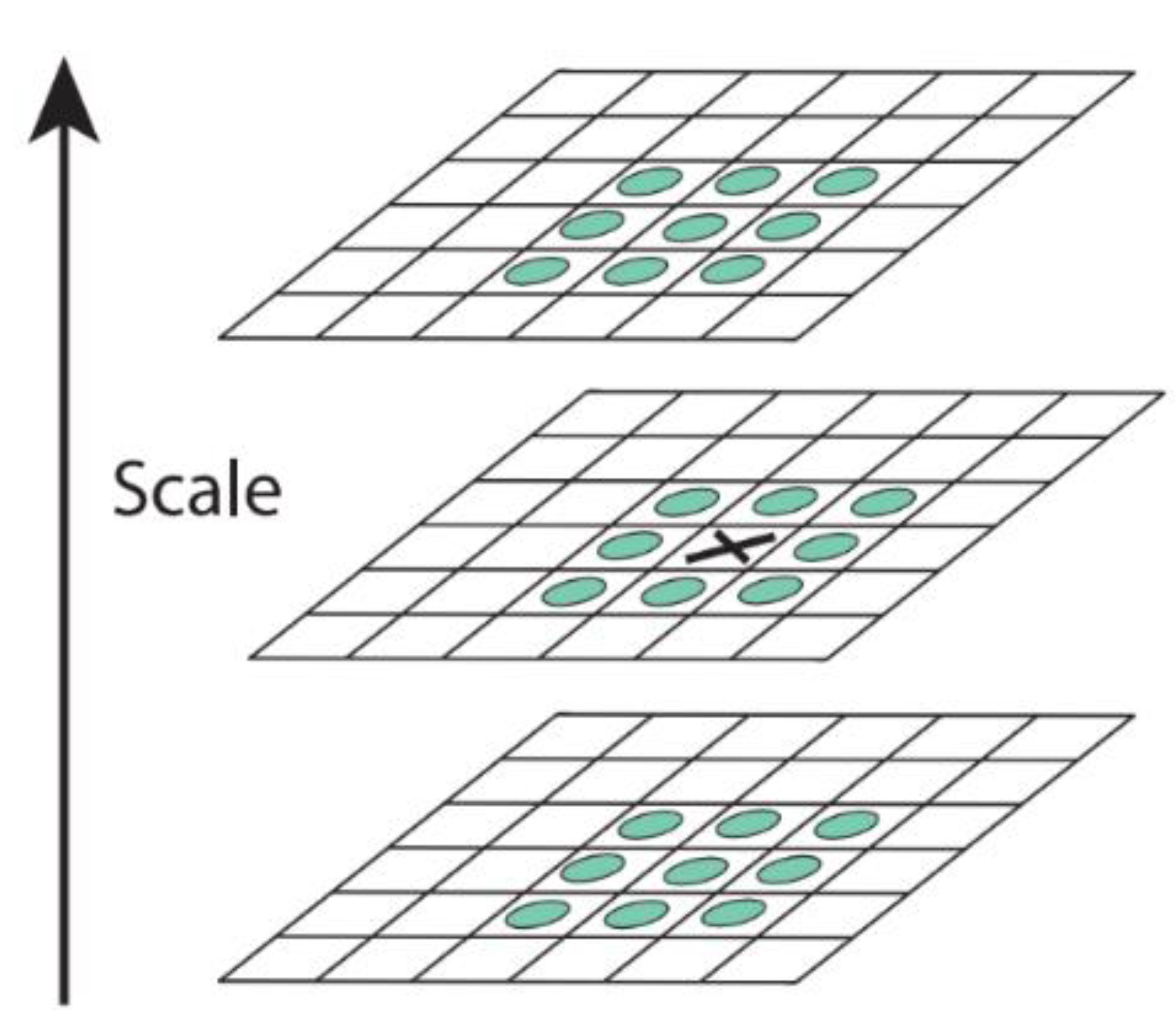
In the Difference of Gaussian pyramid (DOG), 8 pixels of 3 × 3 around the pixel are compared with 18 pixels of 3 × 3 in the upper and lower scales of the same group (Octave), a total of 26 pixels in the neighborhood. In the case of max/min value, this point is regarded as a candidate feature point. See Figure 6.
The Gaussian difference space formula can be expressed as Equation (11):
D x , y , σ = G x , y , k σ G x , y , σ × I x , y = L x , y , k σ L x , y , σ
where, k is the scale coefficient of the Gaussian scale space.
(3)
Locating the key points
When the feature points are determined, the position direction of the feature points must be confirmed in order to realize the rotation invariant feature of the image. Since the extracted feature points are points in discrete space, the key points in real space need more accurate interpolation calculation to reach the position. For function f x , the three-ternary two-order Taylor expansion of its DOG function is represented by Equation (12):
D X = D X 0 + 𝜕 D T 𝜕 X X + 1 2 X T 𝜕 2 D 𝜕 X 2 X
where, X is the position vector, and the deviation size of the extreme point can be obtained at D X = 0 . Equation (13):
X ¯ = 𝜕 2 D 1 X 𝜕 X 2 𝜕 D X 𝜕 X
According to the set threshold, the extreme points of low contrast are eliminated, and the main direction of feature points is found according to the amplitude. Equations (14) and (15):
m x , y = L x + 1 , y L x 1 , y 2 + L x , y + 1 L x , y 1 2
θ x , y = tan 1 L x , y + 1 L x , y 1 / L x + 1 , y L x 1 , y
where, m x , y is the gradient amplitude and θ x , y is the gradient direction.
(4)
Generating the feature description
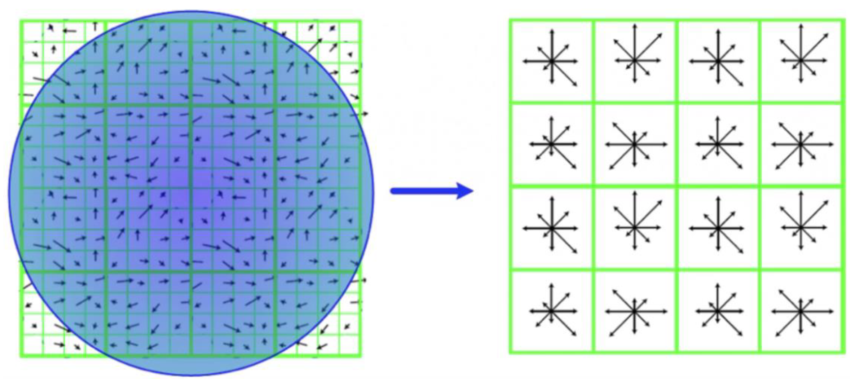
After determining the main direction of the feature points, the neighborhood where the feature points are located was divided into 4 × 4 sub-regions, and each sub-region divided into 8 directions in the 360° range class. Summing the gradient amplitudes in each direction of each region is calculated according to the above formula, and the 128-dimensional vector obtained is the final feature descriptor [46]. The process is shown in Figure 7.

2.5. Traditional Algorithm Classification

The experimental operating system was Windows 10, Pytorch (San Francisco, CA, USA) deep learning framework was adopted, and Python was selected as the programming language. Hardware environment: 8 GB RAM, Intel® Core™ i5-9400F processor, and NVIDIA GeForce RTX 2060 SUPER GPU. Software environment: Compute Unified Device Architecture (CUDA10.2), CUDA Deep Neural Network (cuDNN10.2), Python3.7.3, Pytorch1.5.1. The experimental operating system is shown in Table 2.
Study the different recognition results of different traditional machine learning algorithms for their diseases. For different data sets, the corresponding parameter settings will be different in the artificial feature extraction stage and algorithm implementation stage. In the experiment, the percentage of training set, validation set and test set is 80%, 10% and 10%, respectively. For other parameter settings, different data sets are taken as objects to set the optimization parameters.
For the recognition of plant physiological diseases and pathological diseases, this part takes vegetable deficient cream lettuce as the research object, and discusses the different recognition effects of traditional machine learning algorithms KNN, SVM, and random forest for disease detection.

2.5.1. K Nearest Neighbor

KNN is a simple classifier that works well for basic recognition problems in machine learning techniques [47]. The classification is achieved by identifying the nearest neighbor to a query example and then makes use of those neighbors for determination of the class of the query [48]. This method is easy to implement and can achieve a relatively good result if the neighbors (k value) are chosen carefully. If k has a different value, the results change. A small k value may result in overfitting in the model, whereas a large k value may require too much computation time.

2.5.2. Support Vector Machine

As a binary classification model, SVM is a linear classifier with maximum spacing, and its learning strategy is to maximize the spacing. For the SVM algorithm, if the data points to be measured are p-dimensional vectors, then the P-1-dimensional hyperplane must be used to distinguish these points. The fundamental goal of the SVM algorithm is to select the hyperplane that can make the distance between the nearest data point and the hyperplane maximum. When the experimental data are linearly separable, SVM can establish an optimal segmentation hyperplane in the original feature space and treat it as a decision plane to maximize the margin between positive and negative samples, and then build a classifier using the experimental training set to classify the sample data. When the data are not linearly separable, SVM uses kernel function to map all the sample data information to a certain high-dimensional space, and then finds an optimal classification hyperplane, so as to isolate the sample data of different categories to realize the classification task [49]. Common SVM kernel functions include linear kernel function, Gaussian kernel function and radial basis kernel function. The penalty coefficient C is a very important parameter of the SVM model, which reflects the tolerance to error. The smaller the penalty parameter C is, the smaller the misclassification penalty will be, which is easy to lead to underfitting, and vice versa.

2.5.3. Random Forest

Proposed by Breeiman [50] in 2001, random forest algorithm is a combination classifier based on multiple decision trees with final voting or averaging for high accuracy and generalization characteristics. The number of trees and the criterion to measure splitting are the key parameters of random forest algorithm. The implementation process of random forest algorithm is as follows: first, the number of trees is determined according to the actual needs; then, the data are sampled independently to train the decision tree. The decision trees are combined and the final classification result is obtained by voting. Because of the introduction of randomness, random forest algorithm is not easy to fall into overfitting.

2.5.4. Data Set Parameter Setting and Training

In the stage of color feature extraction, two feature extraction methods, color histogram and color moments, are used at the same time, including the first three moments (mean value, standard deviation and slope) of the color moment method in the single-channel image (R, G and B), and the parameter of the color histogram is set to bucket = 32 to statistically calculate three different single-channel color information. For texture feature extraction, GLCM and LBP are used. The step size of the gray level co-occurrence matrix is set to 1 (step = 1), and the gray level image after preprocessing is calculated in four different directions (0°, 45°, 90°, 135°, respectively) of the four eigenvalues (angular second moment, entropy, contrast, correlation). In order to better extract the local features of disease, in the feature extraction stage, in addition to the color and texture features, SIFT features are also extracted. Since the number of feature descriptors of each image is different when extracting SIFT features of disease images, before the classification task of the classifier, this paper divides the SIFT feature operators into 800 classes by K-means clustering algorithm, to construct the SIFT feature description vector with a length of 800 for each sample image.
In the implementation stage of the algorithm, the parameter settings of different traditional machine learning algorithms are determined through several comparative experiments. For the KNN algorithm, the value of k is set to 5, and the recognition effect is better than other set values. For the SVM algorithm, radial basis kernel function was selected in this paper, and the penalty parameter C was set to 100 according to the cross-validation method. For the random forest algorithm, the number of trees is set to 24 and the criterion is set to entropy by using the Grid Search CV search algorithm. In order to reasonably evaluate the performance of different traditional machine learning algorithms for plant disease recognition, this study used Accuracy, Precision, Recall and F1-score to evaluate the recognition results.

2.6. Deep Learning Methods for Classification

The experimental operating system for the deep learning algorithm was the same as for the traditional algorithm, as shown in Table 2.

2.6.1. Data Augmentation

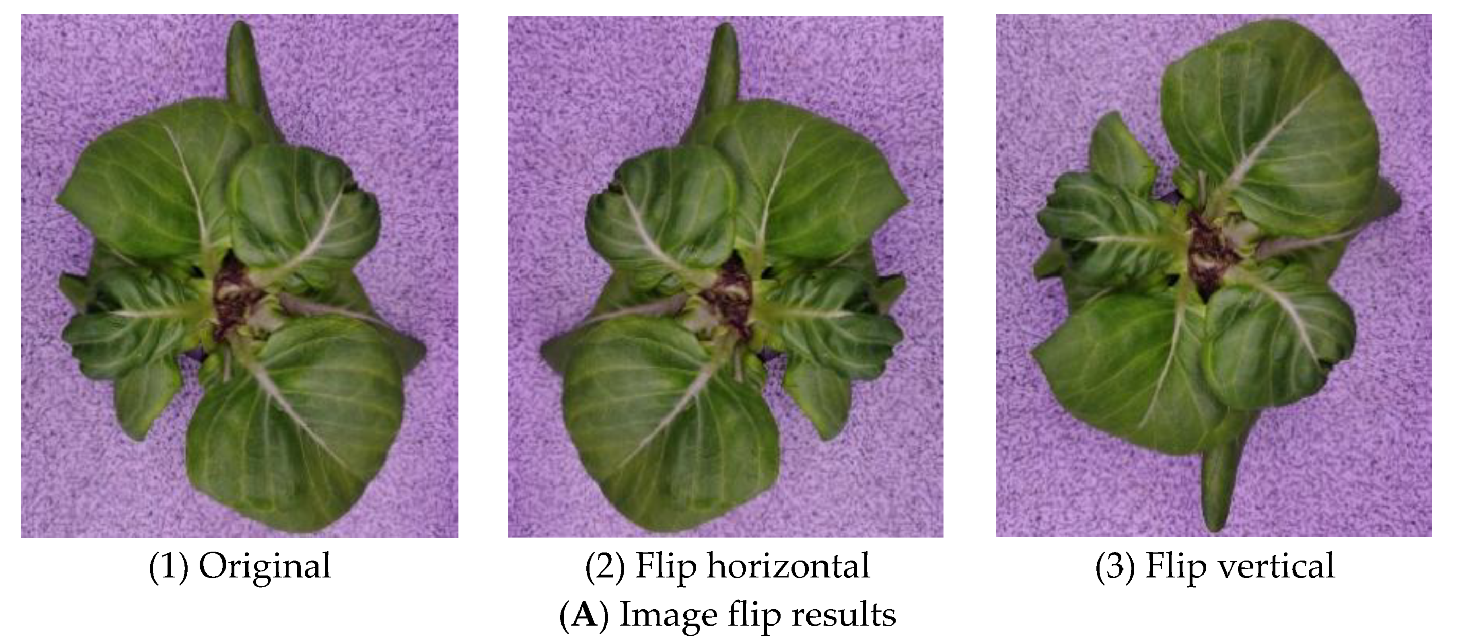
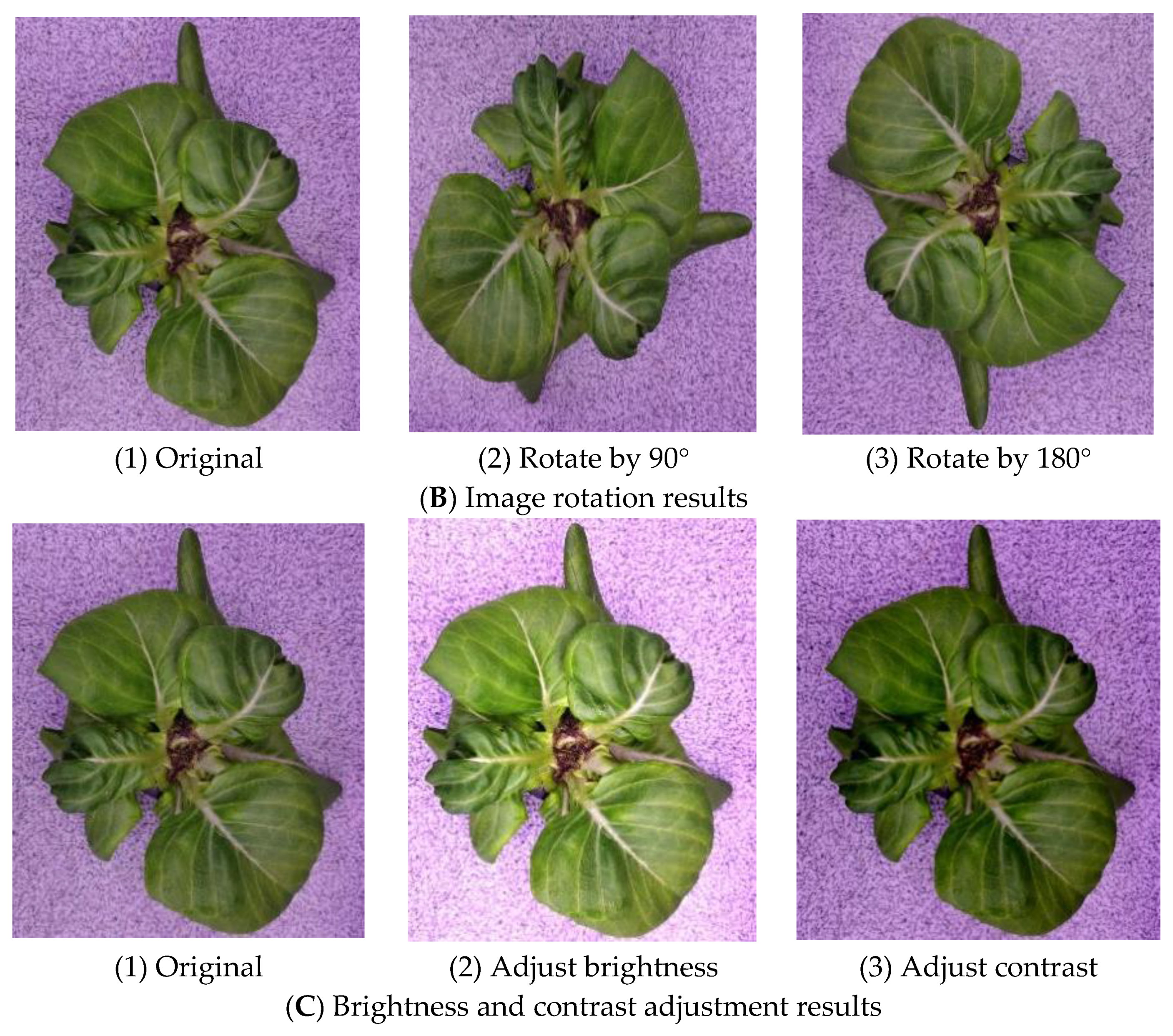
Different from traditional machine learning algorithms, deep learning algorithms usually need large-scale training data to reach ideal conclusions, otherwise it is easy to lead to overfitting problem. Based on the whole plant lettuce as the research object, its deficiency characteristics of image, the experimental data were taken in the plant factory environment, by using the image to flip, rotate, adjust the brightness, and contrasts such as lettuce deficiency after the background segmentation image improve the diversity of image data.
Image flipping can be divided into horizontal and vertical. In order to simulate the images taken in different directions in the environment, the disease images were expanded by random transformation rotation operation. Adjust the image brightness by randomly increasing or decreasing the RGB pixel values and increase or decrease the RGB pixel values based on the intermediate value of image brightness. Enhance the image contrast by enlarging the difference between larger RGB pixel values and smaller RGB pixel values in the image. The augmented images are shown in Figure 8.
The quantity distribution of lettuce prime deficiency data before and after enlargement is shown in Figure 9.

2.6.2. Convolutional Networks Recognition Algorithm Selection

Convolutional neural networks (CNNs) have different performances on datasets in different scenes. In this paper, network selection is mainly considered based on (1) low computational complexity of network model, and (2) good anti-overfitting performance of network. Based on the computational power and memory size of the experimental platform, the identification network model is required to have less parameter calculation and redundancy. In addition, compared with large-scale data sets such as PlantVillage, ImageNet and Kaggle, the lettuce data set established in this paper has a small sample size, which may cause overfitting problems during network training. Therefore, this study also requires the model to have good anti-overfitting performance.
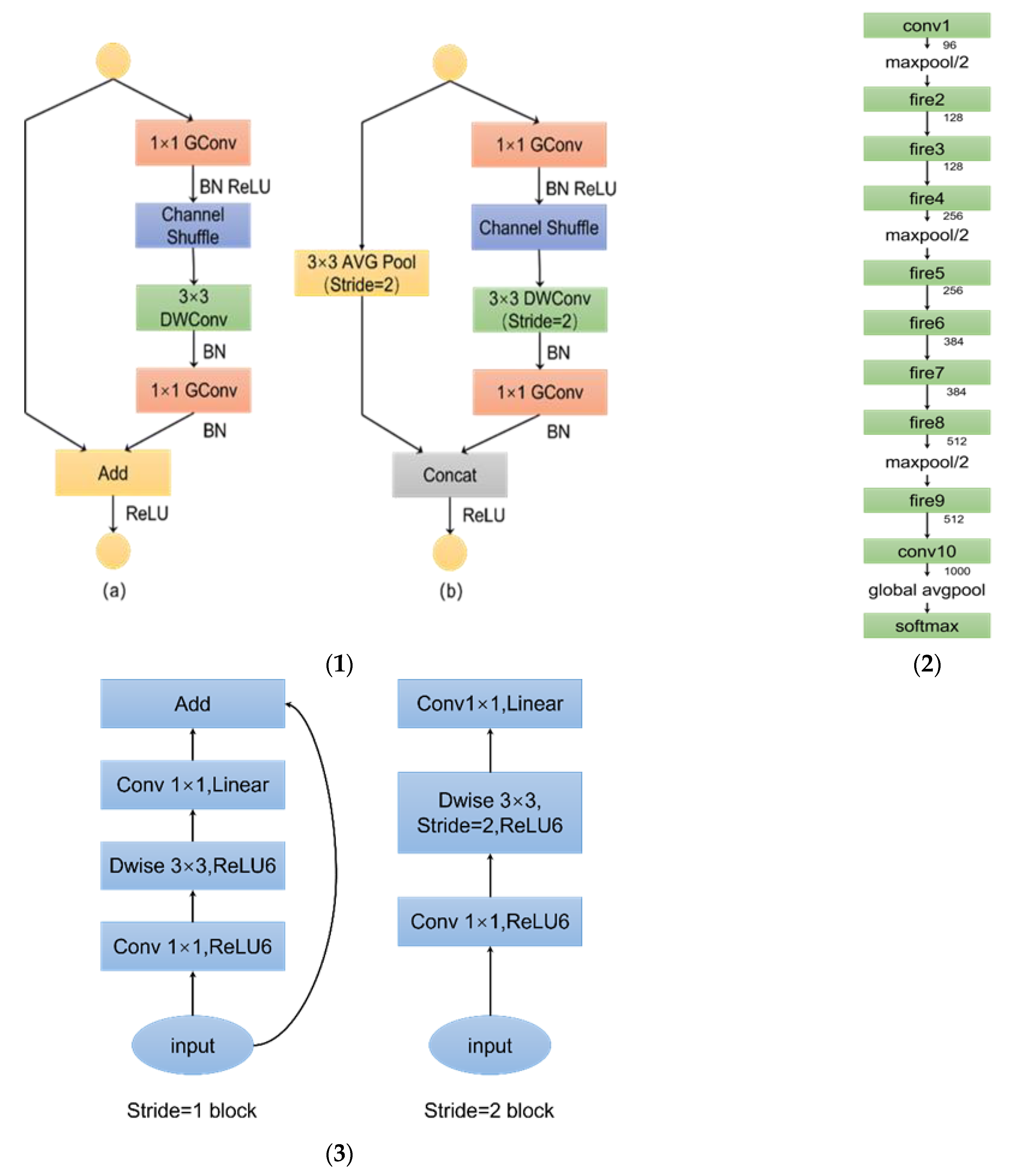
Based on the above analysis, the lightweight networks MobileNet, SqueezeNet and ShuffleNet were finally selected for plant disease recognition. Basic block diagram of MobileNetV2, SqueezeNet and ShuffleNet are shown in Figure 10.
For ShuffleNet, on the basis of the residual unit, the dense 1 × 1 convolution is replaced with a 1 × 1 group convolution. A channel shuffle operation is added after the first 1 × 1 convolution. The rectified linear unit (ReLU) activation function is not used after the 3 × 3 depthwise convolution. For residual units, if the stride is equal to 1, the input and output shapes can be directly added. However, when the stride is equal to 2, the channel number increases while the feature map size decreases, causing a mismatch between input and output. In general, a 1 × 1 convolution can be used to map the input to the same shape as the output. However, in ShuffleNet, a different strategy was adopted, as shown in the Figure 10(1b): using a 3 × 3 average pool with stride = 2 for the original input to obtain a feature map of the same size as the output, and then concatenating the resulting feature map with the output instead of adding it up. The main purpose of doing so is to reduce computational complexity and parameter size.
For SqueezeNet, use the following three strategies to reduce design parameters:
(1)
Use 1 × 1 Convolutional substitution 3 × 3 convolution: the parameters are reduced to 1/9 of the original.
(2)
Reduce number of input channels: this section is implemented using squeeze layers.
(3)
Delay down-sampling operation to provide a larger activation map for convolutional layer: a larger activation map preserves more information and provides higher classification accuracy.
Among them, (1) and (2) can significantly reduce the number of parameters, and (3) can improve accuracy when the number of parameters is limited. SqueezeNet starts with a convolutional layer (conv1), then uses 8 fire modules (fire 2–9), and ends with a convolutional layer (conv10). The numbers of filters in each fire module gradually increase, and a max pooling with a step size of 2 is used after layers conv1, fire4, fire8, and conv10, which places the pooling layer in a relatively backward position. This uses the above strategy (3).
The biggest highlight of MobileNetV2 is inverted residuals and linear bottlenecks. First use 1 × 1 convolution to achieve dimensionality increase, and then through 3 × 3 DW convolution, finally through 1 × 1 convolutional implementation for dimensionality reduction. Convolutional implementation for dimensionality reduction. ReLU6 is used as a nonlinear activation function because it is more robust in low precision calculation. At the same time, 3 × 3 convolution kernel is used as the size of the standard convolution kernel. Dropout and BN are added during training.
The hyper-parameters are shown in Table 3. The initial learning rate is set as 0.0001. To ensure the nonlinearity of the model, ReLU is used as the activation function after the convolution operation. The appropriate batch-size is set for each recognition model according to the model size and video memory capacity limits. The batch size of the model was 256, and the iteration was 30 rounds. Momentum was 0.99. The cross-entropy loss function was selected as the objective function, and the Adam algorithm was adopted as the optimization algorithm.
(1)
Cross-entropy loss function
The cross-entropy loss function is adopted as the loss function of the plant disease recognition model, and its function expression is as follows Equation (16):
L = 1 n x y ln α + 1 y ln 1 α
where, x represents the sample, y represents the true label, α represents the predicted output, and n represents the total number of samples.
(2)
Adam optimization algorithm
Compared to other optimization algorithms, the Adam algorithm is easy to implement, requires less memory, has faster convergence speed, and is invariant to diagonal rescaling of the gradient [52]. Therefore, the Adam algorithm is used to train the convolutional neural network via back propagation in the deep learning algorithm. The calculation formula of the Adam optimization algorithm’s parameter update process is in Equations (17)–(21):
m t = μ × m t 1 + 1 μ × g t
n t = ν × n t 1 + 1 ν × g t 2
m t ^ = m t 1 μ t
n t ^ = n t 1 ν t
θ t + 1 = θ t η n t ^ + ε × m t ^
where, m t and n t are the first-moment estimation and second-moment estimation of the gradient, respectively; m t ^ and n t ^ modify m t and n t , respectively; η n t ^ + ε represents the learning rate; and θ t + 1 is the parameter updating formula of the model.

3. Results and Discussion

3.1. Lettuce Images and Image Features

3.1.1. Channel Separation

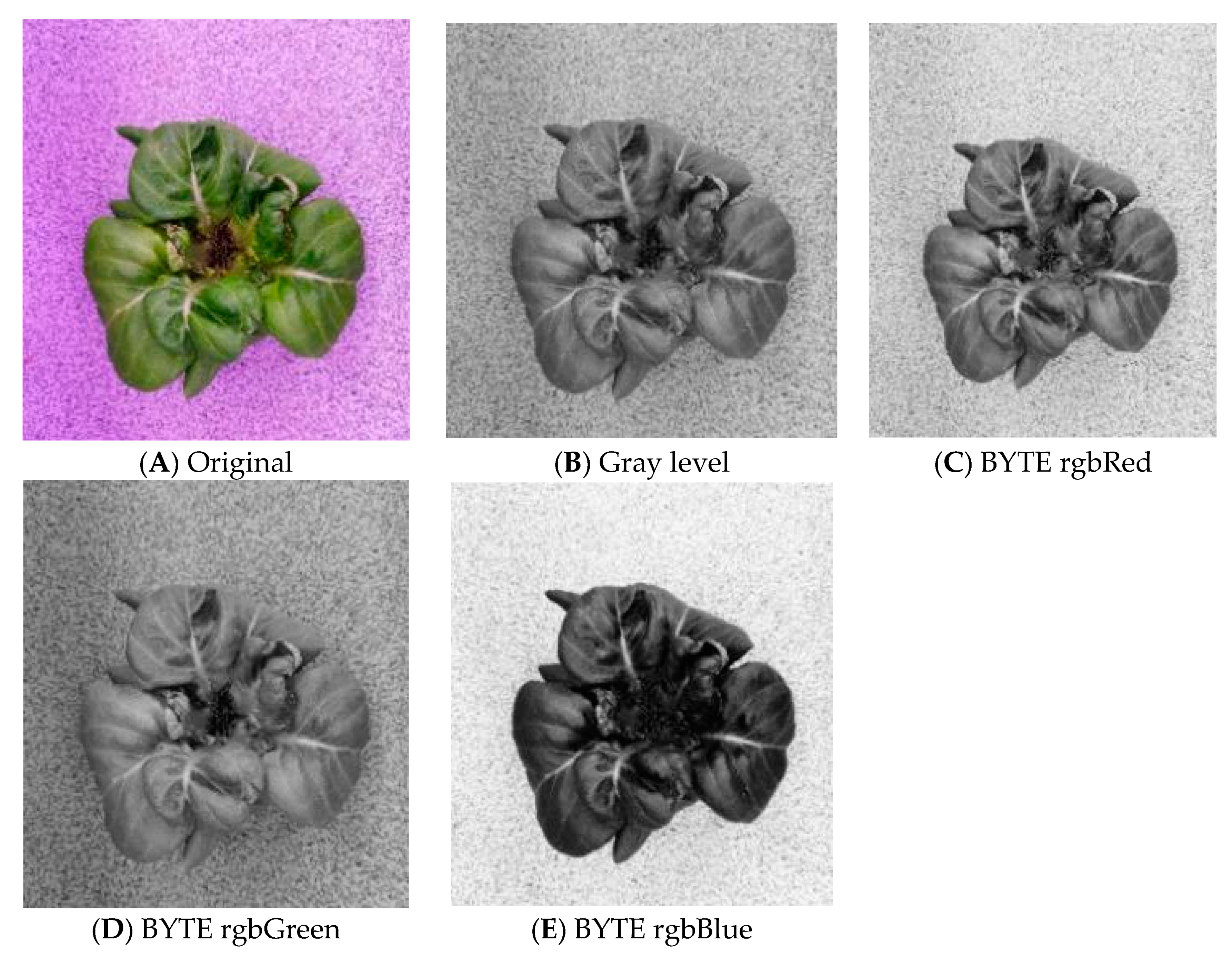
To reduce the influence of complex backgrounds on recognition results, the color images were first converted to grayscale, and then we carried out the corresponding processing methods to improve the image segmentation effect. In order to compare the processing effects of channel separation and direct conversion of images to grayscale images, their processed images are shown in Figure 11.
It can be seen from Figure 11 that the gray image obtained from the blue component had the least background interference, and the image target was more prominent than other gray images, so the gray image extracted from the blue component was used in the study.

3.1.2. Image Filtering

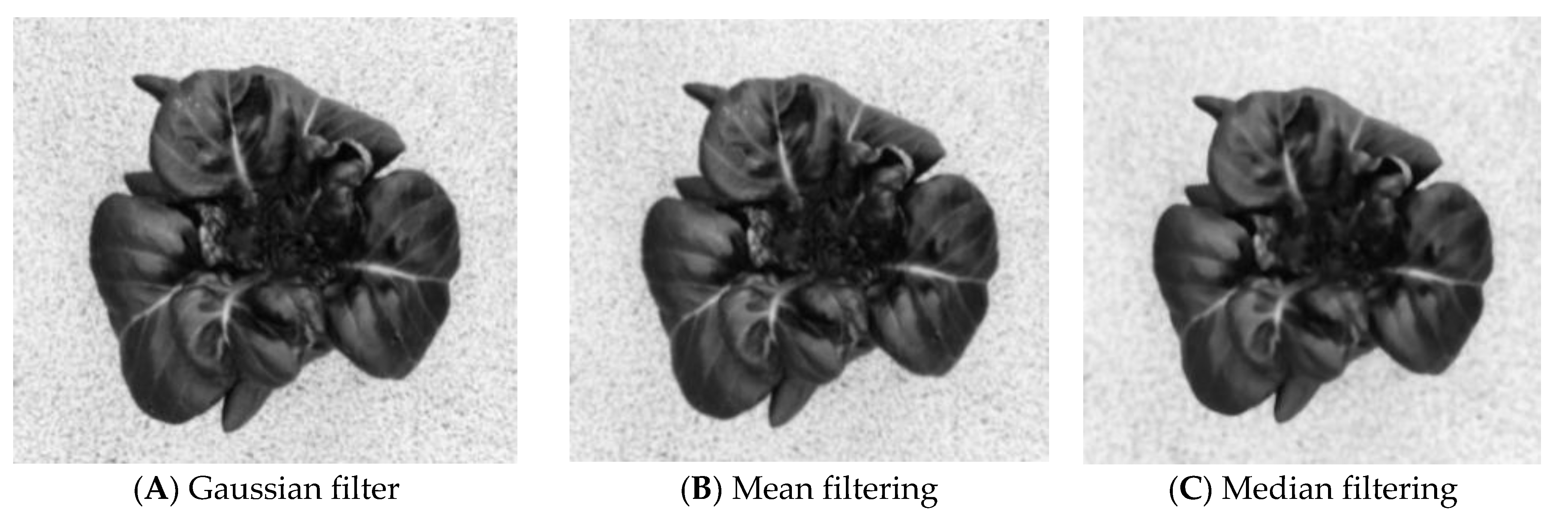
Gaussian filtering, mean filtering and median filtering were performed on the gray level image of the blue component extracted previously, as shown in Figure 12. It is found by comparison that the median filtering can play a very good role in suppressing the point noise and interference pulse, and can ensure that the image target boundary is not blurred with less noise.

3.1.3. Gray Level Transformation

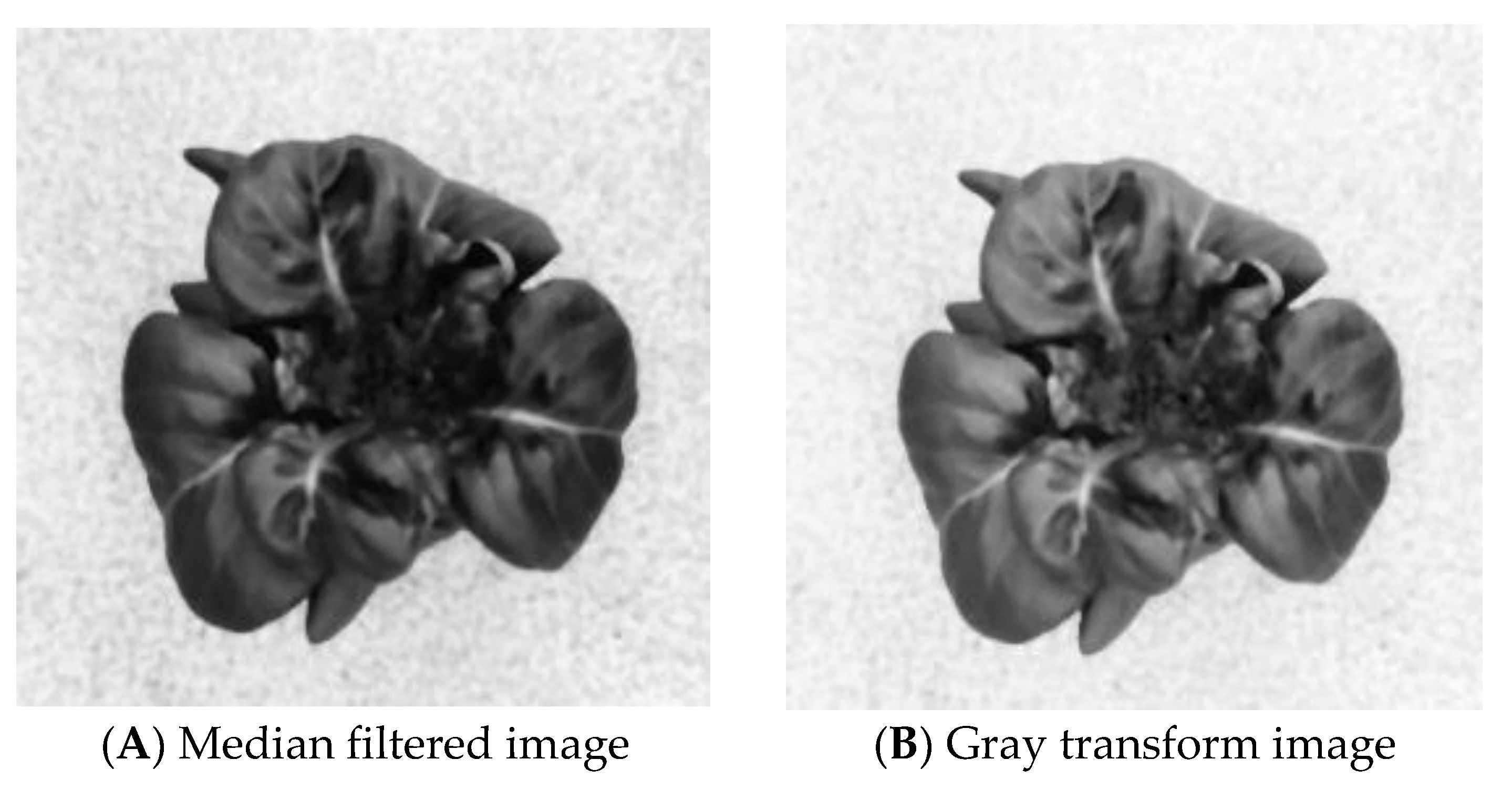
Grayscale transformation can expand the dynamic range and improve image contrast to highlight key information [43]. In order to achieve the goal of highlighting the area of interest in the image and suppressing the gray area of interest in the image, this paper compares a variety of linear gray level transformations and nonlinear transformations, and finds that the gamma transformation is the best when the gamma value is 0.6, which reduces the background interference while making the disease characteristics clearer, as shown in Figure 13.

3.1.4. Threshold Segmentation

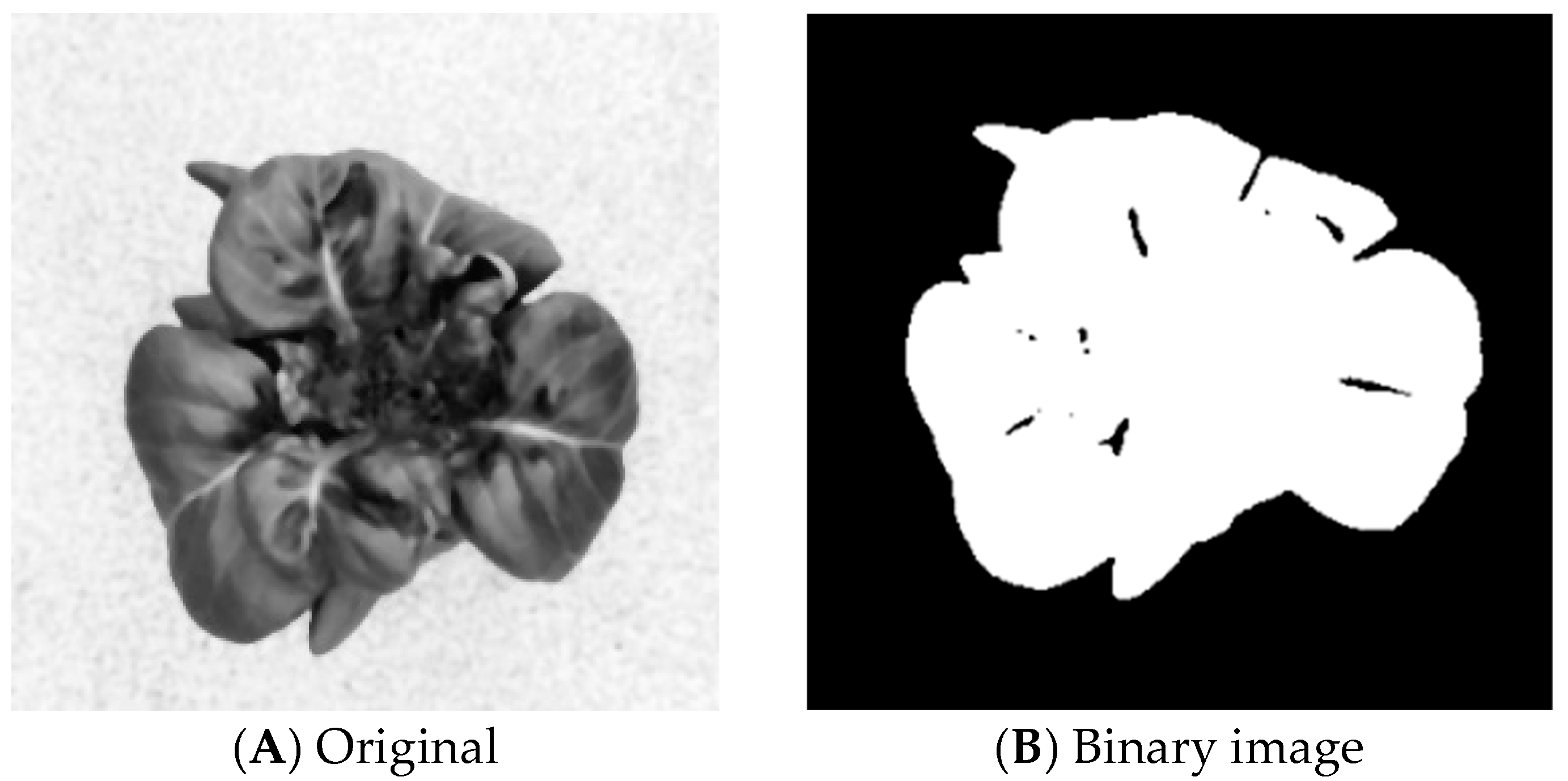
Generally, the target to be extracted from the image is different from the background in terms of gray value. The threshold segmentation method takes full advantage of this feature and regards the image to be segmented as the foreground area and background area with different gray levels. The reasonable threshold is selected through experiments to compare and determine whether the pixels in the image belong to the background area or the foreground area, thus generating the corresponding binary image to achieve the separation of target and background. After threshold segmentation, the binary image obtained is shown in Figure 14.

3.1.5. Foreground Cut and Scale

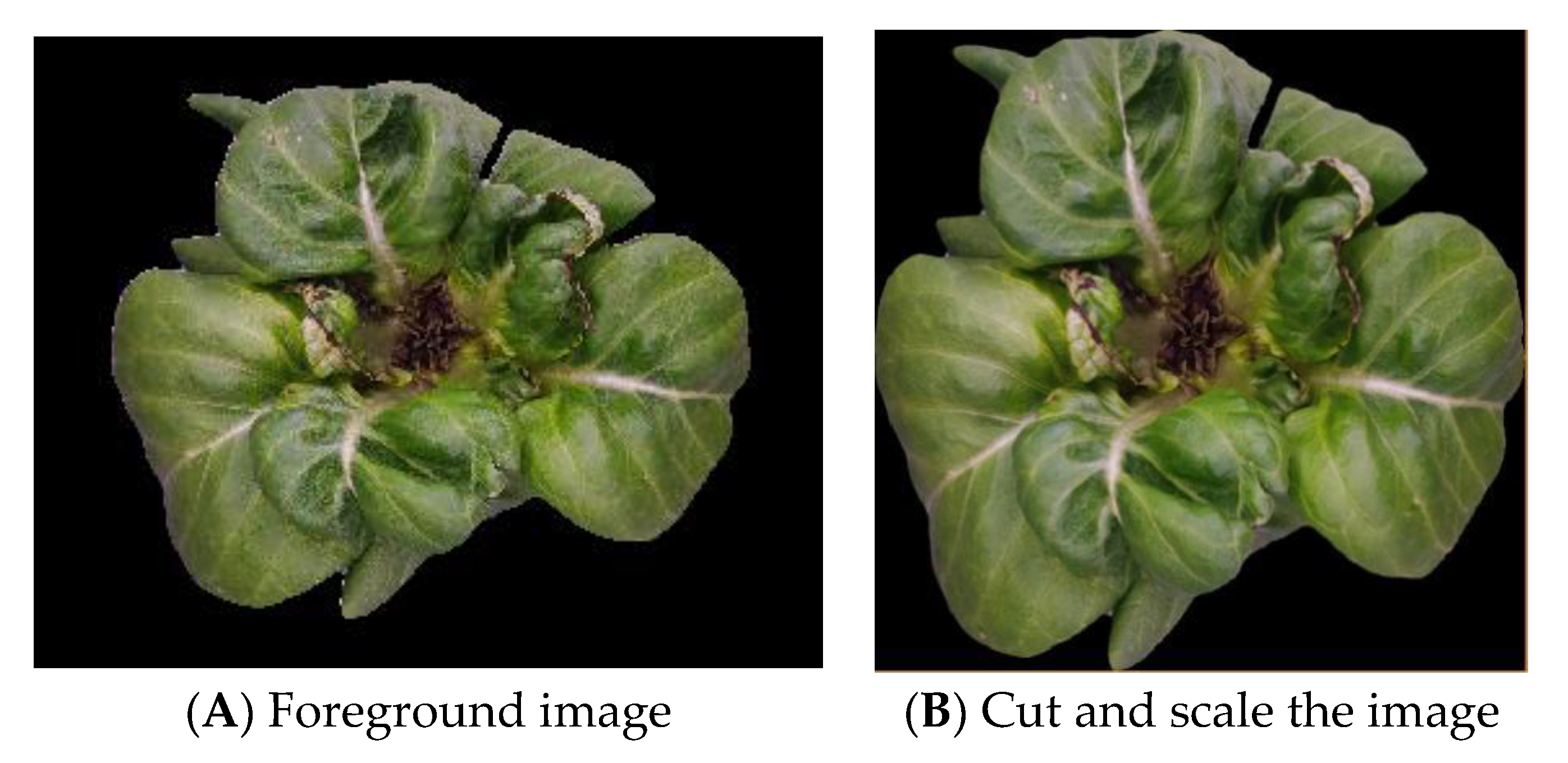
To avoid background interference, unnecessary background features are extracted in the feature extraction stage, and model training is accelerated. At the last stage of pre-processing, the disease image is cut foreground and scaled, and the image is uniformly scaled to 512 × 512 size. The processing result is shown in Figure 15.

3.2. Evaluation Index of Machine Learning Algorithm

This article mainly uses evaluation indicators like accuracy, precision, recall, and F1 score to measure the recognition performance of the model. Among them, Accuracy (Equation (22)) represents the percentage of all correctly classified samples out of all samples; Precision (Equation (23)) represents how many samples that are judged to be positive are true positive samples; Recall (Equation (24)) indicates how many true samples in the sample have been accurately determined; and the F1-score (Equation (25)) value is the harmonic average of accuracy and precision.
Accuracy:
A c c u r a c y = T P + T N T P + F P + T N + F N
Precision (P):
P r e c i s i o n = T P T P + F P × 100 %
Recall (R):
R e c a l l = T P T P + F N × 100 %
F1-score (F):
F 1 = 2 P R P + R × 100 %
Among them, TP (True Positive) represents the number of positive samples correctly identified as positive, TN (True Negative) represents the number of negative samples correctly identified as negative, FP (False Positive) represents the number of negative samples incorrectly identified as positive, and FN (False Negative) represents the number of positive samples incorrectly identified as negative.

3.3. Classification Methods with Different Feature Extraction

In Table 4, the results are displayed as tuples (recall percentage, F1-score percentage) with two significant digits. Under different feature extraction methods, different lettuce nutrient deficiency physiological diseases have different recognition results. The identification of calcium deficiency in color, color + GLCM and color + GLCM + LBP was the best. Magnesium deficiency was best identified in color + LBP, color + GLCM and color + GLCM + LBP. Potassium deficiency was best identified in color. CK is best recognized in color. By comparing all extracted features, including color, gray level co-occurrence matrix (GLCM) and local binary mode (LBP), it is found that color, color + GLCM and All (color + GLCM + LBP) have achieved better recognition results than other methods, and the difference in recognition accuracy between the three methods is very small. Considering the size of feature dimensions, color had the smallest feature dimension, so it was determined as the final feature extraction scheme for lettuce element deficient data set.
Table 5 shows the performance of the three machine learning algorithms used for identification of lettuce nutrient deficiency disease under the optimal feature extraction method (color). For the same dataset, random forest had a slightly better accuracy compared with the other two algorithms. The recognition result is that the accuracy rate is 97.6%, the precision rate is 97.9%, the recall rate is 97.45%, and the F1 score value is 97.6%. The recognition results of the SVM and KNN algorithms for lettuce nutrient deficiency disease were close, but lower than random forest.
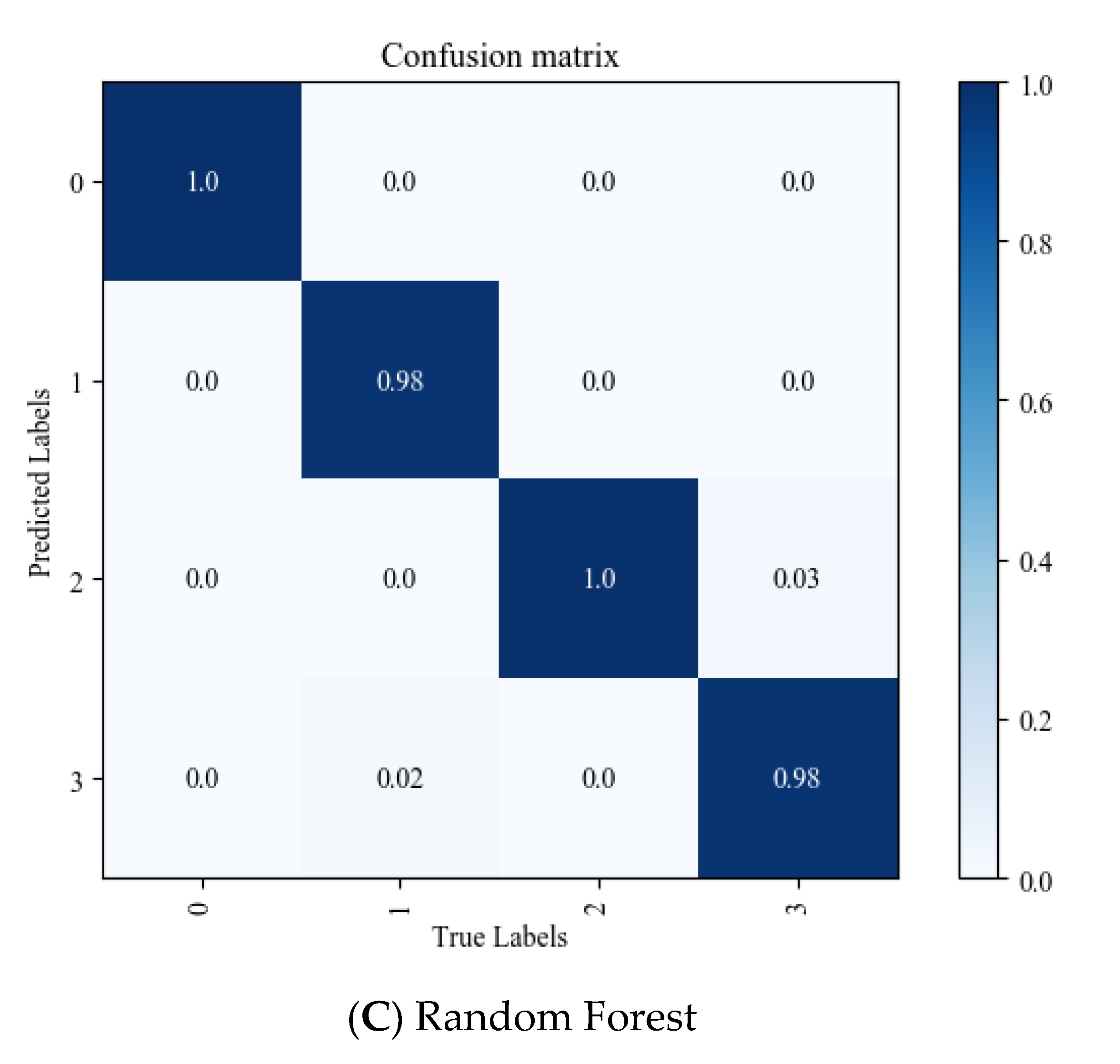
Figure 16 shows the confusion matrix of three traditional machine learning algorithms used for lettuce nutrient deficiency disease classification. It can be seen from the figure that the traditional machine learning algorithm used in this paper can accurately identify the different nutrient deficiencies of lettuce. The possible reason is that compared with other data sets [53], lettuce has fewer nutrient deficiency types (4 types), and the recognition task is simpler. At the same time, different nutrient deficiency types of lettuce have significantly different nutrient deficiency characteristics, and will not interfere with each other as between similar disease types [48].

3.4. Classification Methods with Different Feature Extraction

Traditional machine learning methods cannot propose targeted feature extraction methods and accurate localization methods of features in combination with plant deficiency characteristics. Deep learning methods used automatic feature extraction without manual feature extraction. Features extracted from original image by adjusting the parameters in the convolution and pooling layers.
Table 6 represents the identification results of different lightweight models for lettuce nutrient deficiency disease. Not only was the accuracy evaluation index used, but also the model parameter quantity Params, model floating point calculation quantity FLOPs and reasoning time. Time is used to comprehensively analyze the lightweight model. It can be seen from the figure that the tested models have achieved good recognition results, and all kinds of evaluation indicators have reached more than 99.5%, so the recognition results were relatively ideal. However, in the data set of this paper, the sources of all kinds of deficient data samples were artificially controlled. If we want to use the model in actual production, we also need to consider increasing the universality of the model, otherwise the model will have a good recognition performance in the laboratory environment, but the effect in practical application is not ideal.
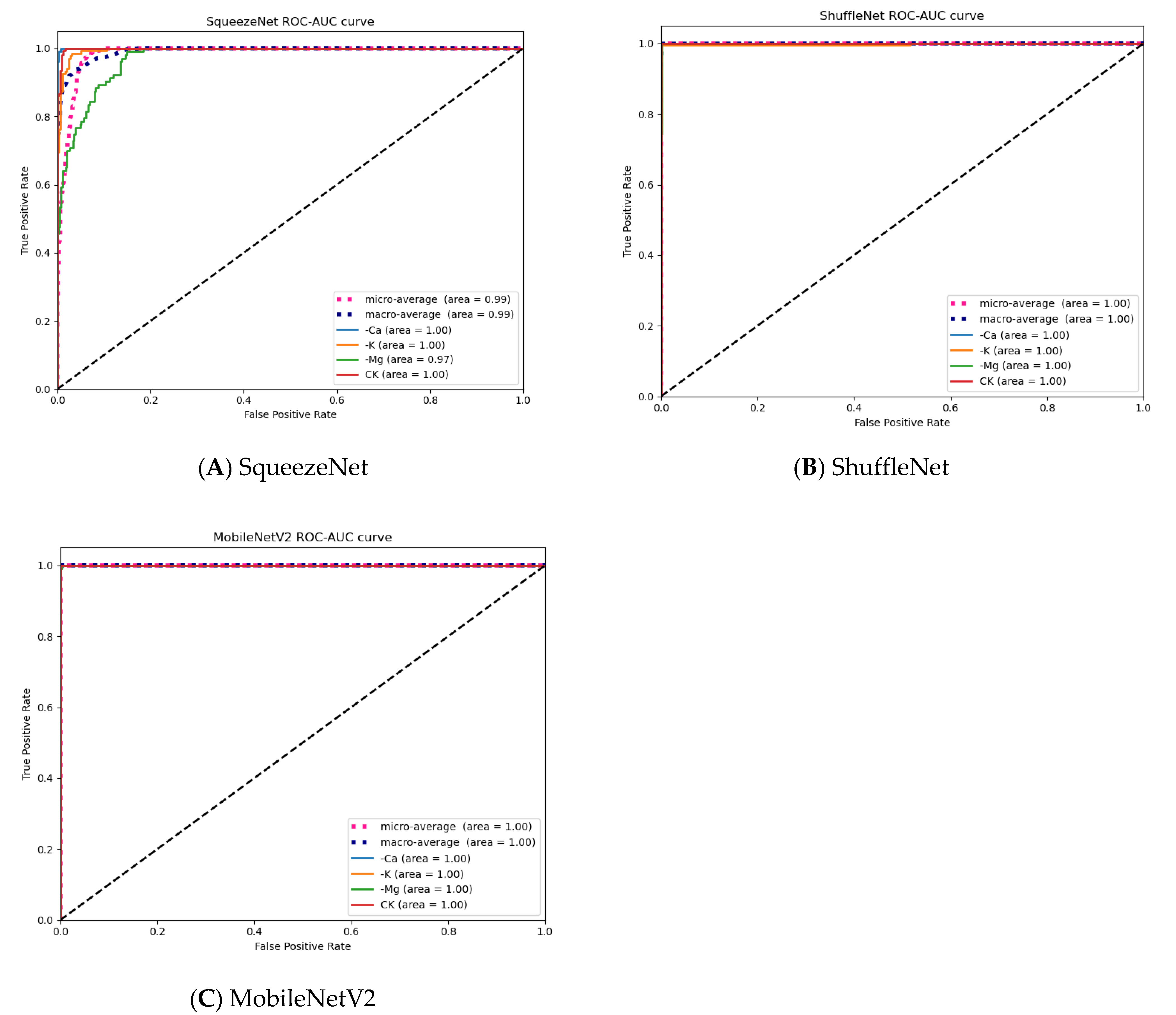
Figure 17 shows ROC (receiver operating characteristic) curve images for each lettuce element deficiency disease under different lightweight classification models. It can be seen from the figure that ShuffleNet and MobileNetV2 have achieved 100% recognition of each element deficiency category, and the classification effect is very ideal, but this is only applicable to the data set obtained in this paper.

3.5. Visualization Evaluation

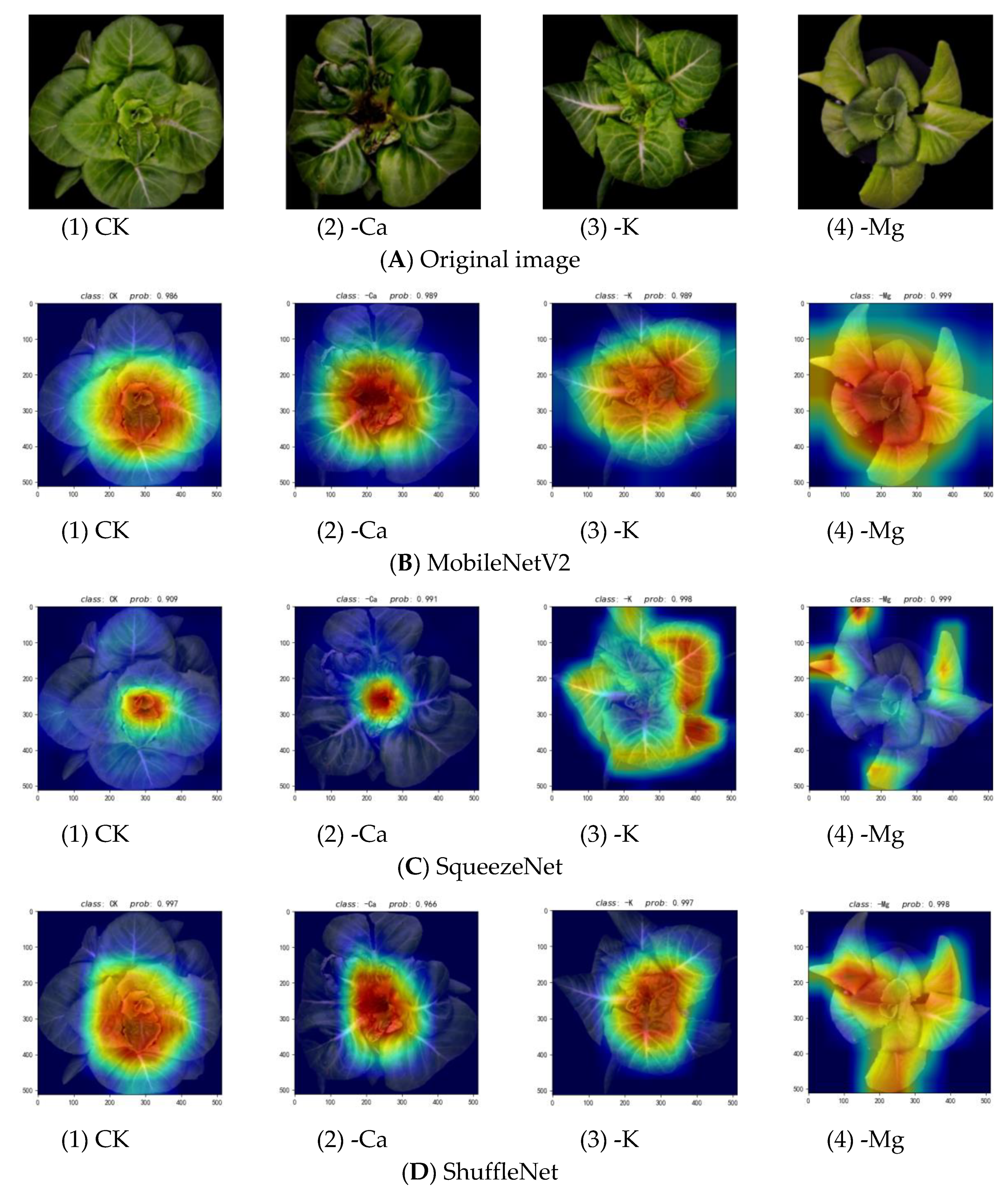
In order to better evaluate the network models, fully understand how they judge disease categories and identify disease locations, we use the feature visualization method to determine if the networks learned “appropriate ” knowledge during network training. We visualize the focused areas in the images. In good classification models, the feature visualization hotspots correspond to the relevant category areas. The darker the color, the more important the area. Figure 18 shows the image of the lightweight model under the gradient class activation mapping feature visualization method.
It can be seen from Figure 18 that for calcium deficiency images, the three lightweight models have accurately extracted the rotten heart disease feature. For the full pixel image, the whole hot spot marker area’s light color indicates no obvious lacking element features in this category, consistent with reality. For the potassium deficient image, only SqueezeNet’s hot area concentrates on the surrounding old leaf area, accurately extracting the interveinal chlorosis deficiency feature. Compared with the SqueezeNet model, the hotspot area of the MobileNet and ShuffleNet classification models is larger, mainly concentrated in the new leaf region without accurate element features. For the magnesium deficiency category, the visualization is the same as potassium deficiency. Only SqueezeNet’s hot area focuses on the small yellow old leaves, while MobileNet and ShuffleNet concentrated more on the whole plant area.

3.6. Discussion

In this paper, machine learning methods were used to detect and identify visible physiological diseases in lettuce. According to the research results of this paper, compared to traditional machine learning algorithms, deep learning algorithms achieved better disease recognition results. The accuracy of the three deep learning models used exceeded 99.5%, and the implementation of deep learning algorithms does not need to manually extract data features like traditional machine learning algorithms. Instead, the network automatically extracts features after data input. That is, a deep learning algorithm is easier to implement than a traditional machine learning algorithm, avoids uncertainty in manual feature extraction, and is more suitable for mobile deployment. Azimi et al. [20], Tenaye et al. [54], and Guerrero et al. [55] all used CNN as the network model and achieve good results. Through comparative experiments, we analyzed the influence of different image feature extraction methods (LBP, GLCM, LBP + GLCM, COLOR, COLOR + LBP, COLOR + GLCM, ALL, SIFT) on the disease recognition effect. We found that the color feature extraction method is the best, Guerrero et al. [55] used the histogram in YUV color space to equalize, and finally converted to RGB color space, to obtain the best result. Table S1 in the supplementary material shows others’ research on plant deficiency.
Therefore, our research results have a certain reliability. Although other studies have some similarities with the work carried out in this paper, they often use single methods for plant diseases identification. We applied both traditional and deep learning methods on the same data set, and used Grad-CAM to visualize pathological sites judged by three lightweight models, making the experimental results more convincing and intuitive. Additionally, lettuce is one of the most common vegetables, and there are few relevant studies, so our study has a certain value and significance as a reference.
In practical, the model could be integrated into mobile applications, intelligent cameras, and other devices for real-time lettuce disease detection and monitoring in plant factories. The models could also be combined with cloud services to achieve large-scale and distributed disease identification systems.

4. Conclusions

In this paper, mobile devices were used to capture images of hydroponic lettuce with different nutrient deficiencies (potassium, calcium, magnesium, and total nutrients) in different growth states in a plant factory. The collected images were preprocessed via median filtering, channel separation, grayscale transformation, and other operations, and then the color, texture and SIFT features of lettuce images were extracted by feature extraction method. Three traditional machine learning algorithms (KNN, SVM, Random Forest) classified the extracted features, and their effects were compared. The results showed that the color feature had the best recognition of lettuce nutrition deficiency diseases, with random forest algorithms achieving the highest accuracy of 97.6% among the traditional methods. At the same time, deep learning algorithms were also used to accurately identify lettuce deficiencies. In order to avoid overfitting of the model, image augmentation technology was used to expand the lettuce dataset. Based on the size and type of data collected, we selected the ShuffleNet, SqueezeNet, and MobileNetV2 lightweight models for recognition. Accuracy, precision, recall, and F1 score were used as model evaluation indicators. The accuracy of all three deep learning models exceeded 99.5%, with ShuffleNet reaching a maximum of 99.9%, indicating ideal recognition results.
Although we have successfully achieved the identification of plant diseases represented by lettuce using traditional machine learning algorithms and deep learning methods. However, there are still some limitations. More datasets are needed to further improve performance, as our datasets size and types were relatively small. The images were idealized in the plant factory. The background lacks complexity, and the problem that harmful features are invisible or may overlap with other features is not considered. In the future, we need to further study these issues.

Supplementary Materials

The following supporting information can be downloaded at: https://www.mdpi.com/article/10.3390/agriculture13081614/s1, Table S1: Studies by others on the plants’ deficiency. References [56,57,58,59,60,61] are cited in the supplementary materials.

Author Contributions

Conceptualization, methodology, data curation, writing—original draft preparation, J.L.; investigation, methodology, writing—reviewing and editing, K.P.; calculations, validation and writing—reviewing and editing, Q.W.; methodology, conceptualization, C.S. All authors have read and agreed to the published version of the manuscript.

Funding

This research was funded by the project of Sichuan Engineering Technology Center (RX2200004133).

Data Availability Statement

Not applicable.

Acknowledgments

We thank Lijuan Tan for her help with this research.

Conflicts of Interest

The authors declare that the research was conducted in the absence of any commercial or financial relationships that could be construed as a potential conflict of interest.

References

  1. Guo, D. Diagnosis of Several Pathological Diseases and Physiological Diseases of Citrus Using Hyperspectral Imaging. Master’s Thesis, Southwest University, Chongqing, China, 2016. [Google Scholar]
  2. Kim, W.-S.; Lee, D.-H.; Kim, Y.-J. Machine vision-based automatic disease symptom detection of onion downy mildew. Comput. Electron. Agric. 2020, 168, 105099. [Google Scholar] [CrossRef]
  3. Varshney, D.; Babukhanwala, B.; Khan, J.; Saxena, D.; Singh, A. Machine Learning Techniques for Plant Disease Detection. In Proceedings of the 2021 5th International Conference on Trends in Electronics and Informatics (ICOEI), Tirunelveli, India, 3–5 June 2021. [Google Scholar]
  4. Fallas-Corrales, R.; van der Zee, S.E.A.T.M. Chapter 42—Diagnosis and management of nutrient constraints in papaya. In Fruit Crops; Srivastava, A.K., Hu, C., Eds.; Elsevier: Amsterdam, The Netherlands, 2020; pp. 607–628. [Google Scholar]
  5. Taha, M.F.; Abdalla, A.; ElMasry, G.; Gouda, M.; Zhou, L.; Zhao, N.; Liang, N.; Niu, Z.; Hassanein, A.; Al-Rejaie, S.; et al. Using Deep Convolutional Neural Network for Image-Based Diagnosis of Nutrient Deficiencies in Plants Grown in Aquaponics. Chemosensors 2022, 10, 45. [Google Scholar] [CrossRef]
  6. Maione, C.; Barbosa, R.M. Recent applications of multivariate data analysis methods in the authentication of rice and the most analyzed parameters: A review. Crit. Rev. Food Sci. Nutr. 2019, 59, 1868–1879. [Google Scholar] [CrossRef]
  7. Takahashi, K.; Kim, K.; Ogata, T.; Sugano, S. Tool-body assimilation model considering grasping motion through deep learning. Robot. Auton. Syst. 2017, 91, 115–127. [Google Scholar] [CrossRef]
  8. Zhang, B.; He, X.; Ouyang, F.; Gu, D.; Dong, Y.; Zhang, L.; Mo, X.; Huang, W.; Tian, J.; Zhang, S. Radiomic machine-learning classifiers for prognostic biomarkers of advanced nasopharyngeal carcinoma. Cancer Lett. 2017, 403, 21–27. [Google Scholar] [CrossRef]
  9. Zhao, Y.; Li, J.; Yu, L. A deep learning ensemble approach for crude oil price forecasting. Energy Econ. 2017, 66, 9–16. [Google Scholar] [CrossRef]
  10. Trang, K.; TonThat, L.; Thao, N.G.M. Plant Leaf Disease Identification by Deep Convolutional Autoencoder as a Feature Extraction Approach. In Proceedings of the 2020 17th International Conference on Electrical Engineering/Electronics, Computer, Telecommunications and Information Technology (ECTI-CON), Phuket, Thailand, 24–27 June 2020; pp. 522–526. [Google Scholar]
  11. Govardhan, M.; Veena, M.B. Diagnosis of Tomato Plant Diseases using Random Forest. In Proceedings of the 2019 Global Conference for Advancement in Technology (GCAT), Bangalore, India, 18–20 October 2019; pp. 1–5. [Google Scholar]
  12. Balakrishna, K.; Rao, M. Tomato Plant Leaves Disease Classification Using KNN and PNN. Int. J. Comput. Vis. Image Process. 2019, 9, 51–63. [Google Scholar] [CrossRef]
  13. Paul, S.G.; Biswas, A.A.; Saha, A.; Zulfiker, M.S.; Ritu, N.A.; Zahan, I.; Rahman, M.; Islam, M.A. A real-time application-based convolutional neural network approach for tomato leaf disease classification. Array 2023, 19, 100313. [Google Scholar] [CrossRef]
  14. Qin, F.; Liu, D.X.; Sun, B.D.; Ruan, L.; Ma, Z.; Wang, H. Image recognition of four different alfalfa leaf diseases based on deep learning and support vector machine. J. China Agric. Univ. 2017, 22, 123–133. [Google Scholar]
  15. Syed-Ab-Rahman, S.F.; Hesamian, M.H.; Prasad, M. Citrus disease detection and classification using end-to-end anchor-based deep learning model. Appl. Intell. 2022, 52, 927–938. [Google Scholar] [CrossRef]
  16. Agarwal, M.; Gupta, S.K.; Biswas, K.K. Development of Efficient CNN model for Tomato crop disease identification. Sustain. Comput. Inform. Syst. 2020, 28, 100407. [Google Scholar] [CrossRef]
  17. Chen, J.; Chen, J.; Zhang, D.; Sun, Y.; Nanehkaran, Y.A. Using deep transfer learning for image-based plant disease identification. Comput. Electron. Agric. 2020, 173, 105393. [Google Scholar] [CrossRef]
  18. Francis, M.; Deisy, C. Disease Detection and Classification in Agricultural Plants Using Convolutional Neural Networks—A Visual Understanding. In Proceedings of the 2019 6th International Conference on Signal Processing and Integrated Networks (SPIN), Noida, India, 7–8 March 2019; pp. 1063–1068. [Google Scholar]
  19. Militante, S.V.; Gerardo, B.D.; Dionisio, N.V. Plant Leaf Detection and Disease Recognition using Deep Learning. In Proceedings of the 2019 IEEE Eurasia Conference on IOT, Communication and Engineering (ECICE), Yunlin, Taiwan, 3–6 October 2019; pp. 579–582. [Google Scholar]
  20. Azimi, S.; Kaur, T.; Gandhi, T.K. A deep learning approach to measure stress level in plants due to Nitrogen deficiency. Measurement 2021, 173, 108650. [Google Scholar] [CrossRef]
  21. Ghosal, S.; Blystone, D.; Singh, A.K.; Ganapathysubramanian, B.; Singh, A.; Sarkar, S. An explainable deep machine vision framework for plant stress phenotyping. Proc. Natl. Acad. Sci. USA 2018, 115, 4613–4618. [Google Scholar] [CrossRef] [Green Version]
  22. Tran, D.; Cédric, C. Early Diagnosis of Iron Deficiency in Commercial Tomato Crop Using Electrical Signals. Front. Sustain. Food Syst. 2021, 5, 631529. [Google Scholar] [CrossRef]
  23. Xu, Z.; Guo, X.; Zhu, A.; He, X.; Zhao, X.; Han, Y.; Subedi, R. Using Deep Convolutional Neural Networks for Image-Based Diagnosis of Nutrient Deficiencies in Rice. Comput. Intell. Neurosci. 2020, 2020, 7307252. [Google Scholar] [CrossRef]
  24. Yi, J.; Krusenbaum, L.; Unger, P.; Hüging, H.; Seidel, S.J.; Schaaf, G.; Gall, J. Deep Learning for Non-Invasive Diagnosis of Nutrient Deficiencies in Sugar Beet Using RGB Images. Sensors 2020, 20, 5893. [Google Scholar] [CrossRef]
  25. Han, X. Research on Recognition Method of Tomato Leaf Deficiency Based on Convolutionneural Network. Master’s Thesis, Northwest A&F University, Xianyang, China, 2022. [Google Scholar]
  26. Rizkiana, A.; Nugroho, A.P.; Salma, N.M.; Afif, S.; Masithoh, R.E.; Sutiarso, L.; Okayasu, T. Plant growth prediction model for lettuce (Lactuca sativa.) in plant factories using artificial neural network. IOP Conf. Ser. Earth Environ. Sci. 2021, 733, 012027. [Google Scholar] [CrossRef]
  27. Hao, X.; Jia, J.; Gao, W.; Guo, X.; Zhang, W.; Zheng, L.; Wang, M. MFC-CNN: An automatic grading scheme for light stress levels of lettuce (Lactuca sativa L.) leaves. Comput. Electron. Agric. 2020, 179, 105847. [Google Scholar] [CrossRef]
  28. Sai, K.; Sood, N.; Saini, I. Classification of various nutrient deficiencies in tomato plants through electrophysiological signal decomposition and sample space reduction. Plant Physiol. Biochem. 2022, 186, 266–278. [Google Scholar] [CrossRef]
  29. Sathyavani, R.; JaganMohan, K.; Kalaavathi, B. Classification of nutrient deficiencies in rice crop using denseNet-BC. Mater. Today Proc. 2022, 56, 1783–1789. [Google Scholar] [CrossRef]
  30. Hamdani, H.; Septiarini, A.; Sunyoto, A.; Suyanto, S.; Utaminingrum, F. Detection of oil palm leaf disease based on color histogram and supervised classifier. Optik 2021, 245, 167753. [Google Scholar] [CrossRef]
  31. Zhang, X.; Zhou, X.; Lin, M.; Sun, J. ShuffleNet: An Extremely Efficient Convolutional Neural Network for Mobile Devices. In Proceedings of the 2018 IEEE/CVF Conference on Computer Vision and Pattern Recognition, Salt Lake City, UT, USA, 18–23 June 2018; pp. 6848–6856. [Google Scholar]
  32. Grigorescu, S.E.; Petkov, N.; Kruizinga, P. Comparison of texture features based on Gabor filters. IEEE Trans. Image Process. 2002, 11, 1160–1167. [Google Scholar] [CrossRef] [Green Version]
  33. Manjunath, B.S.; Ma, W.Y. Texture features for browsing and retrieval of image data. IEEE Trans. Pattern Anal. Mach. Intell. 1996, 18, 837–842. [Google Scholar] [CrossRef] [Green Version]
  34. Wu, C.-M.; Chen, Y.-C.; Hsieh, K.-S. Texture features for classification of ultrasonic liver images. IEEE Trans. Med. Imaging 1992, 11, 141–152. [Google Scholar] [CrossRef]
  35. Haralick, R.M.; Shanmugam, K.; Dinstein, I. Textural Features for Image Classification. IEEE Trans. Syst. Man Cybern. 1973, SMC-3, 610–621. [Google Scholar] [CrossRef] [Green Version]
  36. Ojala, T.; Pietikainen, M.; Harwood, D. Performance evaluation of texture measures with classification based on Kullback discrimination of distributions. In Proceedings of the 12th International Conference on Pattern Recognition, Jerusalem, Israel, 9–13 October 1994; Volume 581, pp. 582–585. [Google Scholar]
  37. Ojala, T.; Pietikäinen, M.; Harwood, D. A comparative study of texture measures with classification based on featured distributions. Pattern Recognit. 1996, 29, 51–59. [Google Scholar] [CrossRef]
  38. Ojala, T.; Valkealahti, K.; Oja, E.; Pietikäinen, M. Texture discrimination with multidimensional distributions of signed gray-level differences. Pattern Recognit. 2001, 34, 727–739. [Google Scholar] [CrossRef] [Green Version]
  39. Ojala, T.; Pietikainen, M.; Maenpaa, T. Multiresolution gray-scale and rotation invariant texture classification with local binary patterns. IEEE Trans. Pattern Anal. Mach. Intell. 2002, 24, 971–987. [Google Scholar] [CrossRef]
  40. Pietikäinen, M. Image Analysis with Local Binary Patterns. In Proceedings of the Image Analysis: 14th Scandinavian Conference, SCIA 2005, Joensuu, Finland, 19–22 June 2005; Springer: Berlin/Heidelberg, Germany, 2005; pp. 115–118. [Google Scholar]
  41. Stricker, M.; Orengo, M. Similarity of Color Images. In Proceedings of the Is&T/Spie’s Symposium on Electronic Imaging: Science and Technology, San Jose, CA, USA, 5–10 February 1995; Volume 2420. [Google Scholar] [CrossRef]
  42. Swain, M.; Ballard, D. Color Indexing. Int. J. Comput. Vis. 1991, 7, 11–32. [Google Scholar] [CrossRef]
  43. Iandola, F.; Han, S.; Moskewicz, M.; Ashraf, K.; Dally, W.; Keutzer, K. SqueezeNet: AlexNet-level accuracy with 50x fewer parameters and <0.5MB model size. arXiv 2016, arXiv:1602.07360. [Google Scholar]
  44. Peng, D.; Deng, A. Improved research on uniform feature extraction based on SIFTalgorithm. Geomat. Spat. Inf. Technol. 2021, 44, 46–50, 56. [Google Scholar]
  45. Lowe, D.G. Distinctive Image Features from Scale-Invariant Keypoints. Int. J. Comput. Vis. 2004, 60, 91–110. [Google Scholar] [CrossRef]
  46. Ding, G.; Qiao, Y.; Yi, W.; Du, L. Improved SIFT extraction and matching based on spectral image space. Trans. Beijing Inst. Technol. 2022, 42, 192–199. [Google Scholar] [CrossRef]
  47. Abdullah, N.E.; Rahim, A.A.; Hashim, H.; Kamal, M.M. Classification of Rubber Tree Leaf Diseases Using Multilayer Perceptron Neural Network. In Proceedings of the 2007 5th Student Conference on Research and Development, Selangor, Malaysia, 11–12 December 2007; pp. 1–6. [Google Scholar]
  48. Tan, L.; Lu, J.; Jiang, H. Tomato Leaf Diseases Classification Based on Leaf Images: A Comparison between Classical Machine Learning and Deep Learning Methods. AgriEngineering 2021, 3, 542–558. [Google Scholar] [CrossRef]
  49. Yang, J.; Qiao, P.; Li, Y.; Wang, N. A review of machine-learning classification and algorithms. Stat. Decis. 2019, 35, 36–40. [Google Scholar] [CrossRef]
  50. Breiman, L. Random Forests. Mach. Learn. 2001, 45, 5–32. [Google Scholar] [CrossRef] [Green Version]
  51. Sandler, M.; Howard, A.; Zhu, M.; Zhmoginov, A.; Chen, L.-C. MobileNetV2: Inverted Residuals and Linear Bottlenecks. In Proceedings of the IEEE Conference on Computer Vision and Pattern Recognition (CVPR), Salt Lake City, UT, USA, 18–23 June 2018. [Google Scholar]
  52. Kingma, D.; Ba, J. Adam: A Method for Stochastic Optimization. In Proceedings of the 3rd International Conference for Learning Representations, San Diego, CA, USA, 7–9 May 2015. [Google Scholar]
  53. Lu, J.; Tan, L.; Jiang, H. Review on Convolutional Neural Network (CNN) Applied to Plant Leaf Disease Classification. Agriculture 2021, 11, 707. [Google Scholar] [CrossRef]
  54. Tenaye, F.; Diriba, C.; Kuyu, M. Coffee Arabica Nutrient Deficiency Detection System Using Image Processing Techniques. Biomed. J. Sci. Tech. Res. 2022, 46, 37600–37606. [Google Scholar] [CrossRef]
  55. Guerrero, R.; Renteros, B.; Castañeda, R.; Villanueva, A.; Belupú, I. Detection of nutrient deficiencies in banana plants using deep learning. In Proceedings of the 2021 IEEE International Conference on Automation/XXIV Congress of the Chilean Association of Automatic Control (ICA-ACCA), Valparaíso, Chile, 22–26 March 2021; pp. 1–7. [Google Scholar]
  56. Luz, P.; Marin, M.; Devechio, F.; Romualdo, L.; Zuñiga, A.; Oliveira, M.; Herling, V.; Bruno, O. Boron Deficiency Precisely Identified on Growth Stage V4 of Maize Crop Using Texture Image Analysis. Commun. Soil Sci. Plant Anal. 2018, 49, 1–11. [Google Scholar] [CrossRef]
  57. Wang, Y.; Hu, X.; Hou, Z.; Ning, J.; Zhang, Z. Discrimination of nitrogen fertilizer levels of tea plant (Camellia sinensis) based on hyperspectral imaging. J. Sci. Food Agric. 2018, 98, 4659–4664. [Google Scholar] [CrossRef]
  58. Bahtiar, A.R.; Pranowo; Santoso, A.J.; Juhariah, J. Deep Learning Detected Nutrient Deficiency in Chili Plant. In Proceedings of the 2020 8th International Conference on Information and Communication Technology (ICoICT), Yogyakarta, Indonesia, 24–26 June 2020; pp. 1–4. [Google Scholar]
  59. Ibrahim, S.; Hasan, N.; Sabri, N.; Abu Samah, K.A.F.; Rahimi Rusland, M. Palm leaf nutrient deficiency detection using convolutional neural network (CNN). Int. J. Nonlinear Anal. Appl. 2022, 13, 1949–1956. [Google Scholar] [CrossRef]
  60. Song, Y.; Liu, L.; Rao, Y.; Zhang, X.; Jin, X. FA-Net: A Fused Feature for Multi-Head Attention Recoding Network for Pear Leaf Nutritional Deficiency Diagnosis with Visual RGB-Image Depth and Shallow Features. Sensors 2023, 23, 4507. [Google Scholar] [CrossRef] [PubMed]
  61. Espejo-Garcia, B.; Malounas, I.; Mylonas, N.; Kasimati, A.; Fountas, S. Using EfficientNet and transfer learning for image-based diagnosis of nutrient deficiencies. Comput. Electron. Agric. 2022, 196, 106868. [Google Scholar] [CrossRef]
Figure 1. Lettuce growth process.
Agriculture 13 01614 g001
Figure 2. Environment of the lettuce deficient experiment.
Agriculture 13 01614 g002
Figure 3. Lettuce samples.
Agriculture 13 01614 g003
Figure 4. Image pre-processing flow chart.
Agriculture 13 01614 g004
Figure 5. Gaussian scale space [45].
Agriculture 13 01614 g005
Figure 6. Key point detection [38].
Agriculture 13 01614 g006
Figure 7. Feature descriptor generation process.
Agriculture 13 01614 g007
Figure 8. The augmented images: flip (A), rotation (B) and brightness and contrast adjustment (C).
Agriculture 13 01614 g008aAgriculture 13 01614 g008b
Figure 9. Distribution of the number of lettuce after data augmentation operation.
Agriculture 13 01614 g009
Figure 10. Basic block diagram of (1) ShuffleNet [31]: (a) ShuffleNet unit with pointwise group1 convolution (GConv) and channel shuffle; (b) ShuffleNet unit with stride = 2; (2) SqueezeNet [43]; (3) MobileNetV2 [51].
Agriculture 13 01614 g010
Figure 11. Image channel separation.
Agriculture 13 01614 g011
Figure 12. Image filtering.
Agriculture 13 01614 g012
Figure 13. Grayscale transformation results.
Agriculture 13 01614 g013
Figure 14. Threshold segmentation result.
Agriculture 13 01614 g014
Figure 15. Foreground clipping and scaling result.
Agriculture 13 01614 g015
Figure 16. Confusion matrix obtained by conventional machine learning algorithms for lettuce deficiency disease identification task (0, 1, 2 and 3 labels in the figure correspond to deficiency species of -Ca, -K, -Mg, and CK, respectively).
Agriculture 13 01614 g016aAgriculture 13 01614 g016b
Figure 17. Area of ROC curve for each deficiency disease under the light models.
Agriculture 13 01614 g017
Figure 18. Area feature visualization images under different light weighting models.
Agriculture 13 01614 g018
Table 1. Deficiency nutrient solution ratios.
ElementsCompoundAll Nutrient Elements Group (CK)/(g/L)Nutrient Deficiency Group/(g/L)
Potassium Depletion
(-K)
Calcium Deficiency (-Ca)Magnesium Deficiency
(-Mg)
Macro elementsCa(NO3)2·H2O0.708450.70845-0.70845
KNO31.001-1.0111.001
NH4H2PO40.40030.40030.40030.4003
MgSO4·7H2O0.492940.492940.49294-
NaNO3-0.84990.50994-
EDTA-2Na (×1000)3.733.733.733.73
FeSO4·7H2O (×1000)2.782.782.782.78
Trace elements (×1000)H3BO30.8660.8660.8660.866
ZnSO4·7H2O0.8630.8630.8630.863
MnSO4·H2O0.8480.8480.8480.848
CuSO4·5H2O0.1750.1750.1750.175
CoCl2·6H2O0.0240.0240.0240.024
(NH4)6MoO24·4H2O0.14410.14410.14410.1441
Table 2. Experimental operating system.
ParametersContent
Operating systemWindows 10
Learning frameworkPytorch1.5.1
Programming languagePython3.7.3
Hardware environment8 GB RAM
Table 3. Hyper-parameters for compared networks.
HyperparameterValue
Learning rate0.0001
The momentum0.99
Batch size256
Epochs30
Table 4. Results for different feature extraction methods with the KNN classifier.
Varieties(Recall Percentage, F1-Score Percentage) of Feature Extraction Methods
LBPGLCMLBP + GLCMcolorColor + LBPColor + GLCMAllSIFT
-Ca(81, 87)(68, 76)(95, 96)(92, 96)(89, 94)(92, 96)(92, 96)(92, 92)
-Mg(68, 71)(71, 76)(81, 88)(97, 97)(97, 98)(97, 98)(97, 98)(90, 95)
-K(88, 84)(79, 74)(95, 89)(99, 97)(99, 94)(99, 95)(99, 96)(99, 90)
CK(85, 86)(87, 89)(87, 91)(98, 98)(93, 95)(95, 96)(96, 97)(87, 93)
average(81, 82)(76, 79)(90, 91)(97, 97)(95, 95)(96, 96)(96, 97)(92, 93)
Table 5. Element deficiency classification results under different traditional machine learning algorithms.
ClassifiersEvaluating Indicator
AccuracyPrecisionRecallF1-Score
KNN97.0%97.1%96.7%96.8%
SVM97.0%96.7%97.2%96.9%
Random Forest97.6%97.9%97.4%97.6%
Table 6. Classification results of lettuce disease with different light weighed models.
AlgorithmsEvaluating Indicator
AccuracyPrecisionRecallF1-ScoreParams/MFLOPs/GTime/ms
ShuffleNet99.9%99.9%99.9%99.8%1.370.0480.89
SqueezeNet99.5%99.5%99.5%99.5%1.240.35238.22
MobileNetV299.8%99.5%99.5%99.5%3.500.3197.12
Disclaimer/Publisher’s Note: The statements, opinions and data contained in all publications are solely those of the individual author(s) and contributor(s) and not of MDPI and/or the editor(s). MDPI and/or the editor(s) disclaim responsibility for any injury to people or property resulting from any ideas, methods, instructions or products referred to in the content.