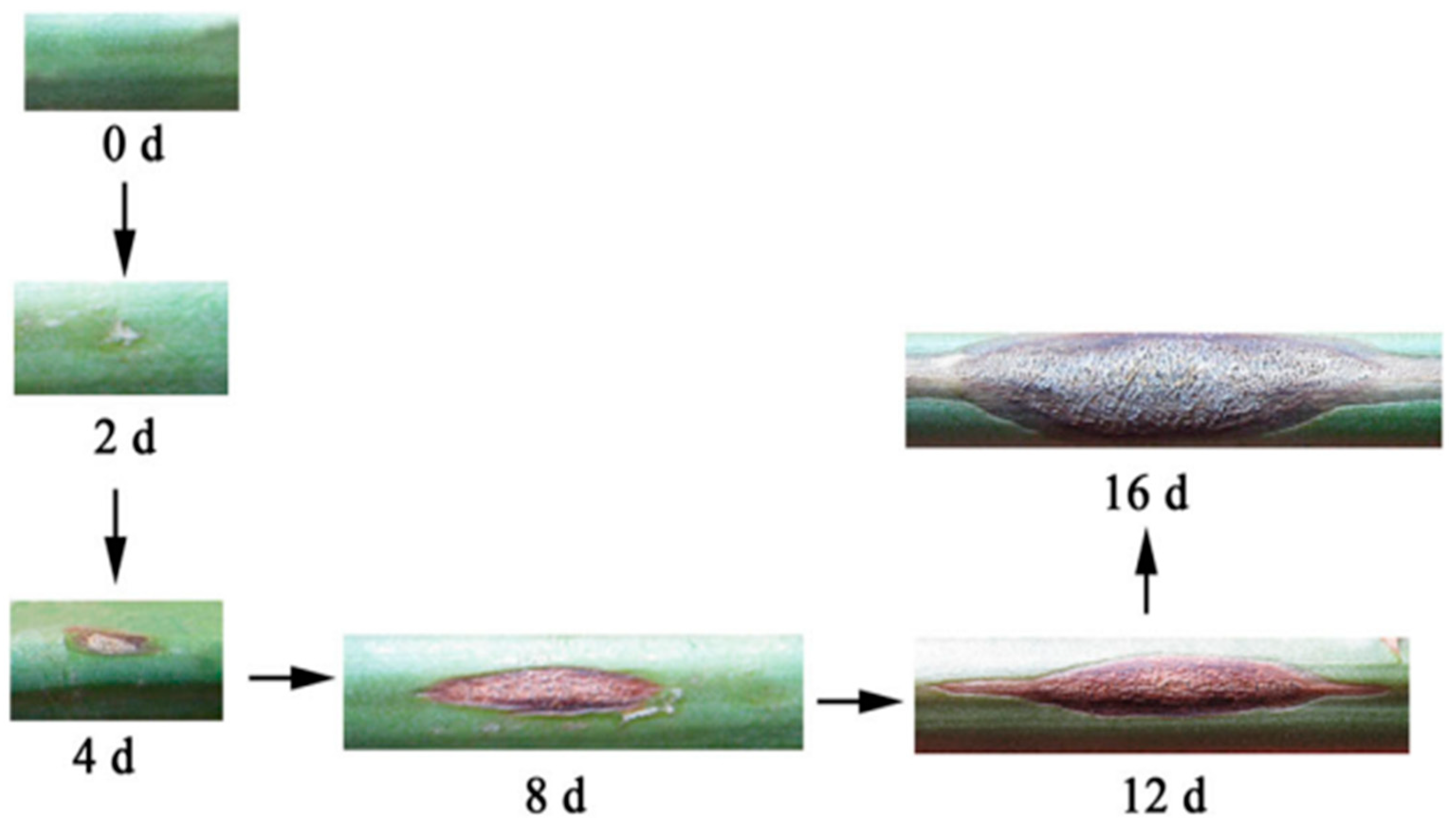
Article

Grading and Detection Method of Asparagus Stem Blight Based on Hyperspectral Imaging of Asparagus Crowns

1
Intelligent Equipment Research Center, Beijing Academy of Agriculture and Forestry Sciences, Beijing 100097, China
2
Nongxin (Nanjing) Smart Agriculture Research Institute Co., Ltd., Nanjing 211800, China
3
National Engineering Research Center of Intelligent Equipment for Agriculture (NERCIEA), Beijing 100097, China
*
Authors to whom correspondence should be addressed.
Agriculture 2023, 13(9), 1673; https://doi.org/10.3390/agriculture13091673
Submission received: 19 July 2023 / Revised: 11 August 2023 / Accepted: 15 August 2023 / Published: 24 August 2023
(This article belongs to the Special Issue Diseases Diagnosis, Prevention and Weeds Control in Crops)

Abstract

:
This study adopted hyperspectral imaging technology combined with machine learning to detect the disease severity of stem blight through the canopy of asparagus mother stem. Several regions of interest were selected from each hyperspectral image, and the reflection spectra of the regions of interest were extracted. There were 503 sets of hyperspectral data in the training set and 167 sets of hyperspectral data in the test set. The data were preprocessed using various methods and the dimension was reduced using PCA. K−nearest neighbours (KNN), decision tree (DT), BP neural network (BPNN), and extreme learning machine (ELM) were used to establish a classification model of asparagus stem blight. The optimal model depended on the preprocessing methods used. When modeling was based on the ELM method, the disease grade discrimination effect of the FD−MSC−ELM model was the best with an accuracy (ACC) of 1.000, a precision (PREC) of 1.000, a recall (REC) of 1.000, an F1-score (F1S) of 1.000, and a norm of the absolute error (NAE) of 0.000, respectively; when the modeling was based on the BPNN method, the discrimination effect of the FD−SNV−BPNN model was the best with an ACC of 0.976, a PREC of 0.975, a REC of 0.978, a F1S of 0.976, and a mean square error (MSE) of 0.072, respectively. The results showed that hyperspectral imaging of the asparagus mother stem canopy combined with machine learning methods could be used to grade and detect stem blight in asparagus mother stems.

1. Introduction

Asparagus officinalis Linn is an important functional vegetable with high nutritional value; it is one of the ten most famous dishes in the world and is known as the “king of vegetables” in the international market [1,2,3]. China is the largest producer and exporter of asparagus in the world. The main stem, lateral branches, sublateral branches, and pseudoleaves of the asparagus mother stem all contain a large amount of chlorophyll, which allows plants to carry out photosynthesis, produce nutrients, and store them in roots underground, providing nutrients for the initiation of young stems. The asparagus mother stem plays a crucial role in the production of asparagus [4,5]. Asparagus stem blight is a devastating soil-borne disease that occurs worldwide. It is called the cancer of asparagus [6]. In some cases, plant blight and yield decrease; in other cases, the whole field is destroyed and yield fails, causing huge losses for asparagus farmers [7,8,9,10]. Asparagus stem blight is caused by Phomopsis asparagi (Sacc.) [11]; once the disease occurs, conidia are released from conidial organs formed on diseased spots of asparagus plants, and then spread to healthy plants through wind and rain, air mist, running water, contact between diseased plants and healthy plants, and contact between pathogenic bacteria in soil or infected residual plants and healthy plants. When the conidia contact with water, they germinate and invade the plant, causing reinfection. Many infections can be formed during the whole growth period of asparagus [6].
The prevention and treatment of asparagus stem blight are mainly based on removing and burning the remnants of diseased plants thoroughly, soil disinfection, fertilization, and pesticide application. Fungicide application starts from the time when the mother stem is retained or before the arrival of the rainy season from July to September and prevents the onset of diseases [6,12]. Fungicides pollute the environment and destroy the ecosystem, and pesticide residues endanger human health [13,14]. Asparagus stem blight is easy to control in the early stage, the amount of application is reduced, and the damage to the plant is less. Therefore, it is very important to explore a rapid, nondestructive, and accurate detection method for stem blight in asparagus mother stems.
Asparagus stem blight mainly affects the stem, and its symptoms are shown in Figure 1. At the beginning of the disease, watery spots appear on the asparagus stem, which expand into fusiform or linear dark brown spots as the disease progresses. Finally, the shape of the spots changes to a spindle shape or oval shape, coloured russet brown in the middle, and depressions and black dots start appearing. Waiting approximately 7 days leads to the drying of asparagus. If the disease is more severe the diseased spots join together and circle the stem, and the affected stem dies and becomes brittle and easily broken [14,15,16].
Conventional methods for the detection of asparagus stem blight mainly include morphological identification, physiological and biochemical identification [17,18], and molecular biological identification [19,20,21]. Morphological identification is subjectively dependent and inefficient [22,23]. Physiological and biochemical identification and molecular biological identification usually have high detection accuracy, but the detection processes are complicated, laborious, time-consuming, inefficient, and cannot meet the needs of the rapid development of modern agriculture. Therefore, it is very important to study rapid, nondestructive, and accurate detection technology for asparagus stem blight [24].
Asparagus stem blight mainly affects the stem, and the asparagus mother stem is occluded by canopy branches and leaves, making it difficult to detect asparagus stem blight. An innovative idea is to identify stem blight by the canopy of the asparagus mother stem, but there is no significant difference in the appearance and morphology between the canopy of healthy and early onset asparagus mother stems and this cannot be recognized by human eyes or RGB images. Visible/near-infrared spectroscopy provides most of the information associated with plant physiological stress [25,26], and the spectral information may be suitable for disease assessment. Hyperspectral images reflect the internal structure, composition information, phenotype texture, and colour morphology of objects. Combined with stoichiometric methods, hyperspectral imaging technology can be used to conduct rapid and nondestructive detection of the comprehensive quality of objects. Hamoud Alshammari [27] proposed an optimal deep learning model to classify olive leaf diseases. A database comprising 3400 olive leaf images was used to train and test the model. The optimal deep learning models, especially DenseNet-GA and ResNet-GA, improved the accuracy rate compared with other machine learning models. Habib Khan [28] proposed an efficient ML-based framework for various kinds of wheat disease recognition and classification to automatically identify the brown- and yellow-rusted diseases in wheat crops. For the comparative analysis of the models, various performance metrics, including overall accuracy, precision, recall, and F1-score, were calculated. Ying Li [29] investigated hyperspectral imaging technology for the fast determination of the hardness and water loss of cucumber. The standard normal variable transformation (SNV) and Savitzky–Golay smoothing (SG) preprocessing methods were compared. Changguang Feng [30] proposed a real-time rice blast disease segmentation method based on a feature fusion and attention mechanism: Deep Feature Fusion and Attention Network (abbreviated to DFFANet). Yuan Shan [31] proposed an improved instance segmentation benchmark Mask R−CNN model to realize an accurate segmentation for the plant leaves; the Cascade R−CNN was also introduced to generate the selection of the proposal boxes for the region proposal network. Zhao Zhang [32] proposed a deep learning-based approach named YOLOv5−CA to achieve the best trade−off between GDM detection accuracy and speed under natural environments; a challenging GDM dataset was acquired in a vineyard under a nature scene (consisting of different illuminations, shadows, and backgrounds) to test the proposed approach.
The aim of this study was to explore a feasible method to identify the disease severity of stem blight based on the canopy of asparagus mother stems. This study will provide method support for the subsequent research of early and even latent period disease detection of asparagus stem blight. It will also provide technical support for the characteristic waveband selection of the stem blight in asparagus and the detection equipment development of the disease grade based on multispectral imaging technology.

2. Materials and Methods

2.1. Hyperspectral Imaging System

A structural schematic diagram of the hyperspectral imaging system is shown in Figure 2, which is mainly composed of a halogen light source, hyperspectral camera, computer, and calibration board. The halogen light source contains two 135 W halogen lamps (Lowel Light Manufacturing Inc., Brooklyn, NY, USA) to provide stable light for the hyperspectral imaging system. The detection wavelength range of SOC 710 Enhanced (Surface Optics Corporation, San Diego, CA, USA) camera is 400~1000 nm, the spectral resolution is 2.34 nm, and the spectral band number is 260. The camera has a built-in push sweep device, and the scanning speed and integration time automatically match, so it can be used to collect hyperspectral images of the canopy of asparagus mother stem plants. The computer (Lenovo, Beijing, China) is mainly used to control the work of the hyperspectral camera, process and analyse the hyperspectral images, and establish the disease grading model of the asparagus mother stem. The function of the calibration board (Surface Optics Corporation, CA, USA) is to calibrate hyperspectral image data. In addition, the system also includes an optical bracket (Lowel Light Manufacturing Inc., NY, USA) for mounting and fixing the hyperspectral camera and light source and a camera dark box(Beijing Shuopin Technology Co., Ltd, Beijing, China) for isolating the interference of external light.

2.2. Asparagus Mother Stem Plants

The asparagus mother stem plants used in this study came from the greenhouse of National Precision Agriculture Research Demonstration Base, Beijing, China and the variety was Chang Geng green asparagus with a seedling age of 3 years (Shouguang Shancheng Agricultural Technology Co. Ltd., Shouguang, China). According to the severity of disease, the asparagus mother stem plants were divided into three grades, as shown in Figure 3. Grade 1: healthy plants with no stem blight symptoms on stem or leaves, 22 plants in total; Grade 2: mild disease plants, with stem blight symptoms on stem, but without symptoms on leaves, 20 plants; Grade 3: moderately and severely affected plants with stem blight symptoms on both stem and leaves, 25 plants. There were a total of 67 asparagus mother stem plants.

2.3. Hyperspectral Image Acquisition and Spectral Data Extraction

The canopy of the asparagus mother stem plant was placed under the hyperspectral camera and the object distance was 45 cm, the aperture of the hyperspectral camera was set to f/5.6, the integration time was set to 35 ms, and the image resolution was 696 × 696 pixels. True-color images of the hyperspectral images of asparagus mother stem canopies of three disease grades are shown in Figure 4. The spectral irradiance in hyperspectral images was converted into spectral reflectance through the calibration of hyperspectral data. ENVI 4.3 software was used to select ten 50 × 50-pixel regions of interest (ROIs) from the canopy region of asparagus mother stem plants in each calibrated hyperspectral image, the average reflectance spectrum of each ROI was extracted as the spectral data for that ROI, and 10 sets of spectral data were extracted from each hyperspectral image. A total of 220 sets of spectral data were extracted from the hyperspectral images of the crown of asparagus mother stem plants in grade 1, 200 sets of spectral data were extracted from the hyperspectral images of the crown of asparagus mother stem plants in grade 2, 250 sets of spectral data were extracted from the hyperspectral images of the crown of asparagus mother stem plants in grade 3, and a total of 670 sets of spectral data were extracted to form the machine learning dataset of this study. From grade 1 to grade 3, each set of spectral data was numbered sequentially, and the spectral data whose numbers were multiples of ‘4’ were selected as the test set, amounting to a total of 167 sets of data. The remaining 503 sets of spectral data were used as the training set and the numbers of spectral data for the three disease grades in the training and test sets are shown in Table 1.

2.4. Spectral Data Preprocessing

The spectral data collected by the hyperspectral camera contain not only the information of the sample but also other irrelevant information and noise, such as electrical noise, sample background, and stray light. Therefore, preprocessing methods aimed at eliminating extraneous information and noise in spectral data become critical and necessary when modelling with chemometric methods. Spectral preprocessing can eliminate baseline drift, rotation, and other noise caused by sample state, measurement conditions, optical scattering differences, and other factors; improve the signal−to−noise ratio of spectral data; retain effective information; reduce background interference; improve the modelling efficiency and the accuracy of model prediction; and enhance the generalization and stability of the model [33]. Different preprocessing methods have different denoising principles and different impacts on the built models. Spectral preprocessing methods are mainly divided into baseline correction, scatter correction, smoothing, signal enhancement, and noise cancellation methods.
First derivative (FD) preprocessing of spectral data can effectively eliminate baseline drift and other background interference, resolve overlapping peaks, improve resolution and sensitivity whilst amplifying the noise, and reduce the signal-to-noise ratio. Before derivative operation, a smoothing operation is needed. Savitzky—Golay smoothing (SG) is a widely used noise reduction method that can effectively eliminate fine white noise in spectral data, but it does not work for low frequency and wide band noise. The standard normal variate (SNV) transformation is used to eliminate the effects of solid particle size, surface scattering, and light path variation on the diffuse reflection spectrum. The detrending treat (DETR) algorithm is often used to eliminate baseline drift in diffuse reflectance spectra. Multiplicative scatter correction (MSC) is mainly used to eliminate the influence of uneven distributions of solid particles, particle size, surface scattering, and optical path changes on the diffuse reflectance spectrum.

2.5. Principal Component Analysis of Spectral Data

The reflectance spectra of the asparagus mother stem canopy were preprocessed using FD, MSC, SG smoothing, etc.
Although the influence of spectral fine white noise, baseline drift, stray light, and so on is eliminated, there are still certain correlations among the 185 variables included in the spectral range of 400–860 nm. When directly used for modelling, not only is the amount of data calculated large, but the calculation speed is slow, and the stability and accuracy of the model are also reduced. Principal component analysis recombines the original numerous variables with a certain correlation into a new set of unrelated comprehensive variables to replace the original variables and converts multiple variables into several comprehensive variables that lose little information. Each principal component is a linear combination of the original variables, and each principal component is not correlated with the others, which gives the principal components superior performance over the original variables [34].
The steps of principal component analysis in this study are as follows:
  • The spectral data matrix A of the asparagus mother stem plant canopy was standardized, and the standardized matrix B was obtained.
The spectral data sample M of the asparagus mother stem plant canopy contains 670 sets of spectral data, M = {X1,X2,X3,……,X670}. Each set of spectral data has 185 spectral reflectance values, X i = { x 1 i , x 2 i , x 3 i , , x 185 i } . The asparagus mother stem plant canopy spectral data matrix A is shown in Equation (1):
A = x 1 1 x 2 1 x 1 2 x 2 2 x 184 1 x 185 1 x 184 2 x 185 2 x 1 669 x 2 669 x 1 670 x 2 670 x 184 669 x 185 669 x 184 670 x 185 670
The mean was calculated as shown in Equation (2):
x n ¯ = 1 670 i = 1 670 x n i   ,   n = 1 ,   2 ,   3 ,   ,   185
The standard error was calculated as shown in Equation (3):
s n = 1 669 i = 1 670 ( x n i x n ¯ ) 2   ,   n = 1 ,   2 ,   3 ,   ,   185
The spectral reflectance values are standardized as shown in Equation (4):
y n r = x n r x n ¯ s n   ,   n = 1 ,   2 ,   3 ,   ,   185
The standardized spectral data matrix B is as shown in Equation (5):
B = y 1 1 y 2 1 y 1 2 y 2 2 y 184 1 y 185 1 y 184 2 y 185 2 y 1 669 y 2 669 y 1 670 y 2 670 y 184 669 y 185 669 y 184 670 y 185 670
2.
The covariance matrix C of spectral data matrix B was calculated.
The covariance is calculated as shown in Equation (6):
cov ( y n i , y n j ) = i = 1 , j = 1 670 , 670 ( y n i y ¯ n ) ( y n j y ¯ n ) 669 , n = 1 , 2 , 3 , , 185
The covariance matrix C is as shown in Equation (7):
C = c o v ( y 1 , y 1 ) c o v ( y 1 , y 2 ) c o v ( y 2 , y 1 ) c o v ( y 2 , y 2 ) c o v ( y 1 , y 669 ) c o v ( y 1 , y 670 ) c o v ( y 2 , y 669 ) c o v ( y 2 , y 670 ) c o v ( y 669 , y 1 ) c o v ( y 669 , y 2 ) c o v ( x 670 , y 1 ) c o v ( x 670 , y 2 ) c o v ( y 669 , y 669 ) c o v ( y 669 , y 670 ) c o v ( y 670 , y 669 ) c o v ( y 670 , y 670 )
The diagonal of matrix C contains the variances of the normalized reflectance y1, y2, , y670 of a certain band, and the nondiagonal elements are the covariances of different normalized reflectances.
3.
The eigenvalues λ and eigenvector μ of covariance matrix C were calculated by using matrix-related knowledge, and the eigenvalues were arranged from large to small.
4.
The eigenvectors were the coefficient vectors of the principal components, and the score of the kth principal component was calculated as shown in Equation (8).
Z k = μ k T C
5.
The contribution rate of the kth principal component was calculated as shown in Equation (9), the cumulative contribution rate was obtained, and the number of principal components was determined.
W k = λ k k = 1 185 λ k
6.
Further statistical analysis was conducted based on the data of principal component scores.

2.6. Disease Classification Modelling Method

2.6.1. KNN Classification

K−nearest neighbour (KNN) is a supervised learning algorithm. The core idea of this algorithm is that if most of the K−nearest neighbour samples in the feature space belong to a certain category, the sample also belongs to this category and has the characteristics of samples in this category. KNN calculates the distance between the feature values of different samples for classification, and the most commonly used metric is the Euclidean distance. K is usually an integer no greater than 20, and if K is too small, the overall model becomes complex and prone to overfitting. A large K value is equivalent to using training samples in a larger region for prediction, which has the advantage of reducing the generalization error, but the disadvantage is that the training error increases. The choice of K value has a significant impact on the results of the algorithm. In this study, after pretreatment and PCA reduction, the principal components of the two sets of spectral data are x = x 1 , x 2 , , x n   and   y = y 1 , y 2 , , y n , the number of principal components is n, and the Euclidean distance between x and y is as shown in Equation (10):
d x , y = k = 1 n x k y k 2

2.6.2. Decision Tree Classification

A decision tree (DT) is a flowchart−like tree structure that classifies sample instances by arranging them from the root node to a leaf node. It is often used in the classification, grading, and early warning system of agricultural diseases [35,36,37]. Each nonleaf node on the tree represents a test for an attribute value, and its branches represent each result of the test. Each leaf node on the tree represents a category of classification; the highest node of the tree is the root node, and the decision tree is constructed in a top-down manner. Starting from the root node of the tree, the attribute values are tested and compared on its internal nodes, and then the corresponding branches are determined according to the attribute values of the given sample. Finally, the conclusions are obtained at the leaf nodes of the decision tree. In this study, the C4.5 algorithm is used to build decision trees through tree generation and tree pruning. After calculating the information gain ratio of each attribute, the attribute with the highest information gain rate is selected to test the attribute of a given set, a recursive algorithm is adopted to establish branches according to the test attribute, and a decision tree is preliminarily obtained.

2.6.3. BPNN Classification

A backpropagation neural network (BPNN) is a kind of multilayer feedforwards neural network that is composed of an input layer, a hidden layer, and an output layer. The main characteristics of BPNNs are forwards transmission of signals and back propagation of error. In forwards signal transmission, the input signal is processed layer by layer from the input layer through the hidden layer until the output layer, and the state of neurons in each layer only affects the state of neurons in the next layer. If the output layer cannot obtain the expected output, it turns to backpropagation and adjusts the network weight and threshold according to the prediction error so that the predicted output of the BPNN keeps approaching the expected output. According to the universal approximation theorem, a continuous function in any closed interval can be approximated using a BPNN with a hidden layer. A three-layer BPNN can complete any N−dimensional to M-dimensional mapping. The number of neurons in the input layer is the same as the dimension of the input data, and the number of neurons in the output layer is the same as the dimension of the output data. The numbers of hidden layer neurons and layers need to be set according to some rules and goals.

2.6.4. ELM Classification

The extreme learning machine (ELM) is a machine learning method based on feedforwards neural network construction with a single hidden layer, which has high working efficiency, high result accuracy, and strong generalization ability. The weights from the input layer to the hidden layer and the bias of the hidden layer of the ELM can be randomly initialized without iterative correction, so part of the computation can be reduced. The weights from the hidden layer to the output layer are obtained by solving a matrix equation. The ELM consists of an input layer, a hidden layer, and an output layer, and its network topology is shown in Figure 5. Among them, the input layer has n neurons, corresponding to n input variables. The hidden layer has l neurons; the output layer has m neurons, corresponding to m output variables.
A training set with Q samples, with input matrix X and output matrix Y, is shown in Equations (11) and (12):
X = x 11 x 12 x 21 x 22 x 1 Q x 2 Q x n 1 x n 2 x n Q n × Q
Y = y 11 y 12 y 21 y 22 y 1 Q y 2 Q y m 1 y m 2 y m Q m × Q
The connection weight between the input layer and the output layer is ω, the connection weight between the hidden layer and the output layer is β, and the threshold value of the neurons in the hidden layer is b, expressed in Equation (13), Equation (14), and Equation (15), respectively:
ω = ω 11 ω 12 ω 21 ω 22 ω 1 n ω 2 n ω l 1 ω l 2 ω l n l × n
β = β 11 β 12 β 21 β 22 β 1 m β 2 m β l 1 β l 2 β l m l × m
b = b 1 b 2 b l l × 1
Suppose the activation function of the hidden layer neuron is g(x); then, the output T of the neural network is as shown in Equation (16):
T = t 1 t 2 t Q 1 × Q ,   t j = t 1 j t 2 j t m j m × 1 = i = 1 l β i 1 g ω i x j + b i i = 1 l β i 2 g ω i x j + b i i = 1 l β i m g ω i x j + b i m × 1  
Among them, j = 1, 2, 3, …, Q, ω i = ω i 1 ω i 2 ω i n ; x j = x 1 j x 2 j x n j T ; and the above formula can be expressed as shown in Equation (17):
H β = T
where T   is the transpose of the matrix T; H is the hidden layer output matrix of the neural network; and its specific form is as shown in Equation (18):
H ω 1 , ω 2 , , ω l , b 1 , b 2 , , b l , x 1 , x 2 , , x Q   =   g ω 1 x 1 + b 1 g ω 2 x 1 + b 2 g ω 2 x 2 + b 2 g ω 2 x 2 + b 2 g ω l x 1 + b l g ω l x 2 + b l g ω 1 x Q + b 1 g ω 2 x Q + b 2 g ω l x Q + b l Q × 1
The goal of single-hidden layer neural network learning is to minimize the output training error, which can approach an arbitrary   ε   > 0 , that is, there are   ω i , β i   ,   and   b i , so that Equation (19) holds.
j = 1 Q | | t j y j | | < ε
In the classification process, once ω i and   b i are randomly determined, then the connection weight β i between the hidden layer and the output layer is uniquely determined, as shown in Equation (20):
β ^ = H + Y
where H + is the Moore–Penrose generalized inverse matrix of the hidden layer output matrix H; therefore, the mathematical model of the ELM can be obtained as shown in Equation (21):
elm X = m i n ω , B , β | | T Y | |

3. Results and Discussion

3.1. Analysis of Spectral Data

Due to the large noise at both ends of the spectral curve, the bands at both ends were removed in this study, and 185 bands ranging from 400 to 860 nm were retained as the effective spectral range. Figure 6 shows the reflection spectral curves of the canopies of each disease grade, Figure 7 shows the curve of the coefficient of variation of the reflection spectral data, and Figure 8 shows the average reflection spectral curves of the canopies of asparagus mother stems of each disease grade. Figure 7 shows that the reflectance spectra of the canopies of asparagus mother stems of the three grades differ greatly in the visible region, and the coefficient of variation peaks at 505 nm green wavelength and 675 nm red wavelength, indicating that the stem blight pathogen affects the absorption of green and red light in the asparagus canopy. From Figure 8, there are differences in the average spectral curves of the canopies of the three types of asparagus mother stems, and the spectral differences of the third grade of moderately and severely affected plants are the most obvious. As the severity of the disease increases, the reflectance of the plants in the near infrared bands gradually decreases.

3.2. Spectral Data Preprocessing

In this study, Savitzky—Golay smoothing (SG), first derivative (FD), detrending (DETR), multivariate scatter correction (MSC), and standard normal variable transformation (SNV) were combined with two or three preprocessing methods to process the spectral data. The derivative order of SG smoothing is ‘0’, the polynomial degree is ‘5’, and the number of smoothing points is ‘25’. The reflectance spectral curves of the canopies of asparagus mother stems after SG and FD pretreatment are shown in Figure 9. The spectral data of the canopies of disease grades 1 and 2 are close to each other, while the spectral data of the canopies of disease grade 3 are significantly different from those of disease grades 1 and 2.

3.3. Results of Principal Component Analysis

In this study, the wavelength range of the effective spectrum was 400~860 nm and included 185 variables. PCA was used for dimensionality reduction. The contribution rates of the principal components were ranked from large to small. When the cumulative contribution rate reached 85%, the principal components involved in the accumulation were taken as the selected principal components. The number of principal components and the score of principal components were determined to reduce the data dimension and eliminate the correlations between variables. The numbers of principal components based on different preprocessing methods are shown in Table 2, Table 3, Table 4, Table 5, Table 6, Table 7, Table 8, Table 9, Table 10, Table 11, Table 12 and Table 13. After the FD preprocessing of the spectral data, PCA was carried out, and a total of 13 principal components were extracted. A two-dimensional space was constructed with principal components 1 (PC1) and 2 (PC2), and the disease grade distribution of 670 sample data points is shown in Figure 10, indicating that the extracted principal components were conducive to disease grading.

3.4. Results of Discrimination Analysis of Disease Grade of Stem Blight in Asparagus Mother Stems

After SG, FD, DETR, MSC, SNV, and two or three kinds of preprocessing, PCA was used to extract the principal components for dimensionality reduction. Based on the principal components, KNN, DT, BPNN, and ELM were used to establish the disease grade discrimination model of the stem blight in asparagus mother stems.

3.4.1. Results of Discrimination Analysis of KNN Disease Grade

Based on the principal component, the KNN method was used to establish a disease grade discrimination model of the stem blight in asparagus mother stems. When K = 4, the discrimination results of the model are shown in Table 2, Table 3 and Table 4. When modeling was carried out based on one preprocessing method, the FD−KNN discrimination model had the best discrimination effect with an ACC of 1.000, a PREC of 1.000, an REC of 1.000, an F1S of 1.000, and a cross-validation error (CVE) of 0.004, respectively, for the test set, while the SG−KNN discrimination model had the worst effect with an ACC of 0.713, a PREC of 0.705, an REC of 0.700, an F1S of 0.697, and a CVE of 0.276, respectively, for the test set. It was indicated that noise interference was eliminated by averaging the reflection spectrum in the region of interest of the hyperspectral image. The effect of SG smoothing on the reflection spectrum data after averaging was not significant, but the baseline drift and other background interference were not eliminated by the reflection spectrum averaging in the region of interest of the hyperspectral image. Therefore, the effect of FD preprocessing was more obvious. When modelling was carried out based on the two pretreatment methods, the model established after the combination pretreatment including FD had a good discrimination effect, whilst the FD−MSC−KNN discrimination model had the best effect with an ACC of 1.000, a PREC of 1.000, an REC of 1.000, an F1S of 1.000, and a CVE of 0.004, respectively, for the test set. The discrimination effects of the SG−SNV−KNN discrimination models were poor with an ACC of 0.778, a PREC of 0.780, an REC of 0.774, an F1S of 0.773, and a CVE of 0.243, respectively, for the test set. When modeling was carried out based on the three combined preprocessing methods, the model established after the combined preprocessing, including FD, had a good discriminative effect; the FD−MSC−DETR−KNN model had the best effect with an ACC of 1.000, a PREC of 1.000, an REC of 1.000, an F1S of 1.000, and a CVE of 0.014, respectively, for the test set, while the SG−MSC−SNV−KNN model had the worst effect. KNN analysis showed that the discrimination effect of the models established after FD pretreatment was good, and the effect of the KNN model established after FD pretreatment was optimal.
After FD−MSC pretreatment and PCA reduction, 12 principal components were extracted from the canopy reflectance spectrum data of asparagus mother stems, and based on the principal components, the FD−MSC−KNN discrimination models of the stem blight grade of asparagus mother stems were established when K = 1, 2, 3, …, 30. Figure 11 shows the influence of the K value on the performance of KNN; a larger K does not necessarily mean a better model. When the K value is less than 4, the discrimination accuracies of both the training set and test set are 1.00. When 5 ≤ K ≤ 13, with the gradual increase in the K value, the grading accuracies of the training set decrease slowly; the grading accuracies of the test set decrease first, then increase, and become stable; and the grading accuracies of both the training set and the test set are greater than 0.95. When K ≥ 14, with the gradual increase in the K value, the grading accuracies of the training set and test set decrease rapidly; when K = 13, there appears a break point in the curve. Figure 11 indicates that it is necessary to comprehensively consider the grading accuracy and the size of the K value. When K = 4, the confusion matrix of the disease grade discrimination results of the test set is shown in Figure 12, and the disease grades discrimination of all samples are correct.

3.4.2. Results of Discrimination Analysis of Disease Grade Using DT

Based on the principal components, the DT method was used to establish the stem blight disease grade discrimination model for asparagus mother stems, and the discrimination effects of the models are shown in Table 5, Table 6 and Table 7. When modeling based on one preprocessing method, the FD−DT discrimination model has the best effect with an ACC of 0.898, a PREC of 0.900, an REC of 0.893, an F1S of 0.895, and a CVE of 0.082, respectively, for the test set, while the SG−DT discrimination model has the worst effect with an ACC of 0.713, a PREC of 0.697, an REC of 0.699, an F1S of 0.697, and a CVE of 0.298, respectively, for the test set. This shows again that noise interference is eliminated by averaging the reflection spectrum in the region of interest of the hyperspectral image. The effect of SG smoothing preprocessing on the averaged reflection spectral data is not significant, but the baseline drift and other background interference are not eliminated, and FD preprocessing to eliminate baseline drift and other background interference is still needed. When modelling is performed based on two pretreatment methods, the FD−MSC−DT discrimination model has the best effect with an ACC of 0.958, a PREC of 0.961, an REC of 0.958, an F1S of 0.959, and a CVE of 0.087, respectively, for the test set. The discrimination effects of the models established after the combination pretreatment including FD are better than when excluding FD. When modelling is carried out based on the three preprocessing methods, the model established after the combined preprocessing including FD has a good discrimination effect. However, the discrimination effects of the models based on the three preprocessing methods are slightly worse than those based on the two preprocessing methods. The discrimination effects for the test set do not increase with the increase in the number of pretreatment methods.
After FD−MSC preprocessing and PCA dimensionality reduction, a total of 12 principal components, namely, 12 attributes, were extracted from the canopy reflection spectral data of asparagus mother stems. A bifurcated decision tree classifier was constructed using the C4.5 decision tree algorithm. The confusion matrix of the disease grade discrimination results of the test set is shown in Figure 13. One healthy sample in grade 1 was misjudged as a moderately and severely diseased sample (grade 3), three mildly diseased samples in grade 2 were misjudged as moderately and severely diseased samples (grade 3), and three moderately and severely diseased samples in grade 3 were misjudged as healthy samples (grade 1).

3.4.3. BPNN Disease Grade Discrimination Analysis Results

Based on the principal components, BPNN was used to establish the stem blight disease grade discrimination model for asparagus mother stems. The discrimination effects of the model in which the number of neurons in the hidden layer was 50 are shown in Table 8, Table 9 and Table 10. When modeling is carried out based on one pretreatment method, the FD−BPNN discrimination model has the best effect with an ACC of 0.946, a PREC of 0.949, an REC of 0.946, an F1S of 0.944, and an MSE of 0.124, respectively, for the test set, while the SG−BPNN discrimination model has the worst effect with an ACC of 0.706, a PREC of 0.751, an REC of 0.710, an F1S of 0.712, and an MSE of 0.350, respectively, for the test set. When modelling is carried out based on two pretreatment methods, the models established after the combination pretreatment including FD have good discrimination effects, and the FD−SNV−BPNN discrimination model has the best effect with an ACC of 0.976, a PREC of 0.975, an REC of 0.978, an F1S of 0.976, and an MSE of 0.072, respectively, for the test set, When modeling is carried out based on three preprocessing methods, the models established after the combined preprocessing, including FD, have good discrimination effects, and the discrimination accuracies of the test set samples are greater than 0.90, and the highest is 0.97. The discrimination effects of the model based on the three preprocessing methods are slightly worse than those based on the two preprocessing methods. The discrimination accuracy of the test set does not increase with an increase in the number of pretreatment methods.
After FD−MSC pretreatment and PCA reduction, 12 principal components were extracted from the canopy reflectance spectrum data of asparagus mother stems. Based on the principal components, BPNN models were established to determine the stem blight grade of asparagus mother stems. The number of neurons in the input layer was 12, the output layer had 1 neuron, the sample number of the training set was 503, the activation function of the neurons in the hidden layer was the tansig function, the transmission function of the output layer was the purelin function, the training function of the back-propagation was the trainlm function, the training frequency was set to 100, the learning rate was set to 0.1, and the training goal was to end the training when the error was less than 0.1. Supposing the number of neurons in the hidden layer n = 1, 2, 3, …, 80, Figure 14 shows the influence of the number of neurons in the hidden layer on the performance of the BPNN. When the number of neurons in the hidden layer was less than 50, the discrimination accuracy of the test set increased slowly with the increase in the number of neurons and gradually levelled off. It is not that the more neurons there are in the hidden layer, the better the model effect. It is necessary to comprehensively consider the discrimination effect of the test set, the model training time, and the number of neurons in the hidden layer and make a compromise. The disease grade discrimination results of the samples in the test set in which the number of neurons in the hidden layer was 50 are shown in Figure 15. All the healthy samples in grade 1 were correctly identified, and one moderately and severely diseased sample in grade 3 was misjudged as a healthy sample (grade 1), three moderately and severely diseased samples in grade 3 were misjudged as mildly diseased samples (grade 2), one mildly diseased sample in grade 2 was misjudged as a mild healthy sample (grade 1), and one mildly diseased sample in grade 2 was misjudged as a moderately and severely diseased sample in grade 3.

3.4.4. ELM Disease Grade Discrimination Analysis Results

Based on the principal components, the ELM method was used to establish the stem blight disease grade discrimination model of asparagus mother stems. The discrimination results of the models in which the number of neurons in the hidden layer was 100 are shown in Table 11, Table 12 and Table 13. When modeling is carried out based on one pretreatment method, the FD−ELM discrimination model has the best effect with an ACC of 0.994, a PREC of 0.995, an REC of 0.993, an F1S of 0.994, and an NAE of 1.000, respectively, for the test set, while the SG−ELM discrimination model has the worst effect with an ACC of 0.749, a PREC of 0.747, an REC of 0.745, an F1S of 0.745, and an NAE of 8.307, respectively, for the test set. When modeling is carried out based on the two pretreatment methods, the model discrimination effects are better, and the discrimination accuracies of the samples in the test set are greater than 0.790; the discrimination effects of the model established after the combination pretreatments, including FD, are better, and the discrimination accuracies of the samples in the test set are greater than 0.970. When modelling is carried out based on the three combined preprocessing methods, the discrimination effect of the models is good, and the discrimination accuracies of the samples in the test set are greater than 0.800; the discrimination accuracies of the models established after the combined preprocessing, including FD, were better, and the discrimination accuracies of the samples in the test set were greater than 0.970.
After FD−MSC pretreatment and PCA reduction, 12 principal components were extracted from the canopy reflectance spectrum data of asparagus mother stems. Based on the principal components, the ELM discrimination model for the stem blight grade of asparagus mother stems was established. The number of neurons in the input layer was 12, the number of neurons in the output layer was 1, the number of samples in the training set was 503, the activation function was the sigmoid function, and the function was continuous and smooth in the definition domain. Suppose the number of neurons in the hidden layer is 10, 20, 30, …, 300. Figure 16 shows the influence of the number of neurons in the hidden layer on the ELM performance; it is not the case that the more neurons there are in the hidden layer, the better the model effect is. When the number of neurons in the hidden layer is less than 60, the discrimination accuracies of the training set and the test set gradually increase with the increase in the number of neurons in the hidden layer. When the number of hidden layer neurons is greater than 60, the discrimination accuracy of the training set and the test set tends to be stable with the increase in the number of neurons in the hidden layer. Therefore, it is necessary to comprehensively consider the discrimination accuracy and the number of neurons in the hidden layer. The disease grade discrimination results of the test set samples in which the number of neurons in the hidden layer was 100 are shown in Figure 17; the disease grades discrimination of all samples are correct.

3.5. Discussion

(1)
In this study, visible/near-infrared hyperspectral imaging technology combined with machine learning was used to detect stem blight through the canopy of asparagus mother stems, and feasible methods to identify disease grade based on the canopy of asparagus mother stems were explored.
(2)
Considering the advantages and disadvantages of various spectral data preprocessing methods and that interference information is often diverse and complex, this research studied the effect of different preprocessing and combination preprocessing methods on the grading detection of stem blight in asparagus mother stems to obtain real and reliable spectral information.
(3)
The SG smoothing preprocessing method selected in this study had no obvious effect on improving the effects of the disease grade discrimination models, mainly because the noise interference had been eliminated when the reflection spectrum in the region of interest discrimination were averaged, as shown in Figure 18, and the averaged spectral curve was much smoother than the raw spectral curve.
(4)
When the KNN and ELM methods were used for modeling, respectively, the model discrimination effects were similar, and the model discrimination effects based on one, two, and three combined preprocessing methods were similar to each modeling method. When using the DT method for modeling, the model discrimination effects based on two and three combined preprocessing methods, respectively, were similar, which was a little better than the model discrimination effects based on one preprocessing method. When using the BPNN method for modeling, the model discrimination effects based on two and three combined preprocessing methods, including FD, respectively, were similar, which was better than the model discrimination effects based on the FD preprocessing methods. In summary, the KNN, DT, ELM, and BPNN model discrimination effects did not increase with the increase in the combination numbers of the preprocessing methods.
(5)
In this study, the modeling methods of KNN and ELM were found to be optimal not only for their excellent modeling effects, but also for their efficient and simple modeling process. KNN worked by measuring the distance between the feature values of different samples. ELM was a single hidden layer neural network with only one neuron in the output layer, and the activation function was a Sigmoid function, therefore they were suitable for the requirements of lightweight models. The spectral data preprocessing method of FD was found to be optimal since it played a prominent role in the KNN, DT, BPNN, and ELM models.
(6)
The results showed that the hyperspectral detection of stem blight based on the canopy of asparagus mother stems was feasible, laying a foundation for subsequent multispectral research and the development of corresponding equipment. This study provides an efficient, accurate, and non-destructive detection method for the disease grading of asparagus stem blight and would strongly promote the development of precision pesticide spraying technology based on disease degree.

4. Conclusions

This study explored the feasibility of detecting asparagus stem blight grades based on the hyperspectral imaging of asparagus mother stem canopy combined with machine learning methods. The effects of different spectral data pretreatment methods and modelling methods on the asparagus stem blight disease grade discrimination model were discussed, and the results of the disease grading were analysed.
(1)
The grading detection of stem blight in asparagus mother stem can be realized based on the combination of the hyperspectral imaging of the asparagus mother stem canopy and machine learning methods, which overcame the difficulty in identifying stem blight in asparagus mother stem with human eyes and RGB images. This method was capable of rapid, accurate, and nondestructive detection, laying the foundation for subsequent multispectral research and the development of corresponding equipment for field applications.
(2)
KNN, DT, BPNN, and ELM were used to establish the discrimination model of asparagus stem blight disease grade. KNN and ELM models had the best discrimination effect and were suitable for the lightweight model requirements of embedded systems. The FD−KNN, FD−MSC−KNN, FD−DETR−MSC−KNN, and FD−MSC−ELM models had a disease grade discrimination accuracy of 1.000 in the test set, and all the disease grades of all samples were identified correctly.
(3)
The FD pretreatment method significantly improves the discrimination effect of the models. When modelling was carried out based on one spectral data preprocessing method, the model established based on FD preprocessing had the best discrimination effect, and the disease grade discrimination accuracies in the test set of the FD−KNN, FD−DT, FD−BPNN, and FD−ELM models were 1.000, 0.898, 0.948, and 0.994, respectively. When modelling was carried out based on two and three combined pretreatment methods, the models established based on the combined pretreatment, including FD, had better discrimination effects. The disease grade discrimination accuracies in the test set of the FD−MSC−KNN, FD−DETR−MSC−KNN, and FD−MSC−ELM models were 1.000, and the disease grades of all samples were correctly identified.

Author Contributions

Conceptualization, C.L.; methodology, X.W.; formal analysis, M.C. and H.L.; data curation, Y.L. and X.Z.; writing—original draft, L.C.; supervision, C.Z. All authors have read and agreed to the published version of the manuscript.

Funding

The support was provided by (1) Jiangsu Province Key Research and Development Program project (BE2021302), (2) Youth Foundation of Beijing Academy of Agriculture and Forestry Sciences (QNJJ202013), and (3) Special project for innovation capacity building of Beijing Academy of agricultural and Forestry Sciences (KJCX20210402).

Institutional Review Board Statement

Not applicable.

Data Availability Statement

The data presented in this study are available on request from the corresponding author.

Conflicts of Interest

The authors declare no conflict of interest.

References

  1. Liu, K.; Lu, Y.; Chen, Y.; Li, S. Biological characters of phomopsis asparagi (SACC.) bubak. Acta Phytopathol. Sinica 1994, 24, 299–304. [Google Scholar]
  2. Joshi, G.; Rawat, M.S.; Bisht, V.; Negi, J.; Singh, P. Chemical constituents of Asparagus. Pharmacogn. Rev. 2010, 4, 215–220. [Google Scholar] [CrossRef]
  3. Takahashi, H.; Yoshida, C.; Takeda, T. Sugar Composition in Asparagus Spears and Its Relationship to Soil Chemical Properties. J. Appl. Glycosci. 2019, 66, 47–50. [Google Scholar] [CrossRef]
  4. Yu, E. The Research of Mother Fern Kept Method and Nitrogen and Potassium Fertilizer Used of Asparagus Cultured in Plastic Greenhouse; Chinese Academy of Agricultural Sciences: Beijing, China, 2015. [Google Scholar]
  5. Shen, W. Changes photosynthetic rate and the contents of nitrogen, phosphorus, and potassium in asparagus officinalis ratoon in autumn. Bull. Sci. Technol. 1992, 111–114. [Google Scholar] [CrossRef]
  6. Sun, Q.; Zhao, F.; Chen, H.; Du, Y.; Shi, N.; Xiao, H.; Yin, C.; Li, X.; Lan, B.; Yang, Y. The Comprehensive Prevention and Control Techniques of Asparagus Stem Blight: Research Progress. Chin. Agric. Sci. Bull. 2023, 39, 108–115. [Google Scholar]
  7. Liu, Z.; Sun, J.; Yang, H.; Mu, L.; Zhang, R. Biological characteristics of phomopsis asparagi the pathogen of asparagus stem blight. J. Shenyang Agric. Univ. 2008, 39, 301–304. [Google Scholar]
  8. Uecker, F.A.; Johnson, D.A. Morphology and taxonomy of species of phomopsis on asparagus. Mycologia 1991, 83, 192–199. [Google Scholar] [CrossRef]
  9. Davis, R.D. Asparagus stem blight recorded in Australia. Australas. Plant Pathol. 2001, 30, 181–182. [Google Scholar] [CrossRef]
  10. Takeuchi, Y.; Kakizoe, E.; Yoritomi, R.; Iwato, M.; Kanno, A.; Ikeuchi, T.; Mori, M.; Murakami, K.; Uragami, A.; Matsumoto, M.; et al. Features in Stem Blight Resistance Confirmed in Interspecific Hybrids of Asparagus officinalis L. and Asparagus kiusianus Makino. Hortic. J. 2018, 87, 200–205. [Google Scholar] [CrossRef]
  11. Yang, Y.; Li, X.; Meng, F.; Lan, B.; Zhang, J. Identification of the pathogen of asparagus stem blight and analysis of its regional difference. J. Plant Prot. 2012, 39, 315–320. [Google Scholar] [CrossRef]
  12. Qu, H.; Cui, G.; Zhang, Y. Research progress on control strategy of asparagus stem blight. J. Chang. Veg. 2021, 18, 45–49. [Google Scholar]
  13. Cheah, L.H.; Horlock, C.M. Field-applied fungicides and postharvest treatments to control Asparagus diseases posing biosecurity threats to New Zealand. New Zealand. Plant Prot. 2007, 60, 94–98. [Google Scholar]
  14. Yang, Y.Q.; Lan, B.; Jian, Y.L.; Chang, D.D.; Zhang, S.L.; Li, X.M. Infection process and pathogenic mechanism of Phomopsis asparagi, the Asparagus stem blight pathogen. Phytoparasitica 2016, 44, 11–18. [Google Scholar] [CrossRef]
  15. Zhang, J.; Liu, D.; Yan, J.; Liu, C.; Shen, X.; Xu, M.; Cui, X. A study progress of phomopsis aspasagi(Sacc.) bubak in China. Beijing Agric. 2012, 12, 104–106. [Google Scholar]
  16. Jia, T.; Liu, C.; Ni, S.; Yin, G. Occurence of stem rot of asparagus and its control. J. Plant Prot. 1992, 19, 111–115. [Google Scholar]
  17. Abdelrahman, M.; Nakabayashi, R.; Mori, T.; Ikeuchi, T.; Mori, M.; Murakami, K.; Ozaki, Y.; Matsumoto, M.; Uragami, A.; Tsujimoto, H.; et al. Comparative Metabolome and Transcriptome Analyses of Susceptible Asparagus officinalis and Resistant Wild A. kiusianus Reveal Insights into Stem Blight Disease Resistance. Plant Cell Physiol. 2020, 61, 1464–1476. [Google Scholar] [CrossRef]
  18. Sun, Q.; Qu, R.; Lan, B.; Yin, C.; Chen, H.; Du, Y.; Shi, N.; Xiao, H.; Li, X.; Yang, Y. Research progress on biological charac-teristics and genetic polymorphism of asparagus stem blight pathogen. J. Shanxi Agric. Sci. 2023, 51, 462–468. [Google Scholar]
  19. Zhang, Y.; Chen, G.; Qu, H.; Zhou, J.; Zhao, P.; Luo, S.; Tang, Y.; Yin, Y. Generation and screening of T-DNA insertion mutants mediated by agrobacterium tumefaciens in the garden asparagus stem blight pathogen phomopsis aspar-agi. Curr. Microbiol. 2017, 74, 1270–1277. [Google Scholar] [CrossRef]
  20. Guo, Y. Preliminary Study on Green Control Technology of Asparagus Stem Blight; Nanjing Agricultural University: Nanjing, China, 2019. [Google Scholar]
  21. Yang, Y.Q.; Sun, Q.; Li, C.M.; Chen, H.F.; Zhao, F.; Huang, J.H.; Zhou, J.S.; Li, X.M.; Lan, B. Biological characteristics and genetic diversity of phomopsis asparagi, causal agent of asparagus stem blight. Plant Dis. 2020, 104, 2898–2904. [Google Scholar] [CrossRef]
  22. Guan, J.; Nutter, F.W. Quantifying the intrarater repeatability and interrater reliability of visual and remote-sensing dis-ease-assessment methods in the alfalfa foliar pathosystem. Can. J. Plant Pathol. 2003, 25, 143–149. [Google Scholar] [CrossRef]
  23. Nutter, F.W.; Esker, P.D.; Netto, R.A.C. Disease assessment concepts and the advancements made in improving the ac-curacy and precision of plant disease data. In European Journal of Plant Pathology; Springer: Dordrecht, The Netherlands, 2006; pp. 95–103. [Google Scholar]
  24. Pethybridge, S.J.; Hay, F.; Esker, P.; Groom, T.; Wilson, C.; Nutter, F.W. Visual and Radiometric Assessments for Yield Losses Caused by Ray Blight in Pyrethrum. Crop. Sci. 2008, 48, 343–352. [Google Scholar] [CrossRef]
  25. Muhammed, H.H. Hyperspectral Crop Reflectance Data for characterising and estimating Fungal Disease Severity in Wheat. Biosyst. Eng. 2005, 91, 9–20. [Google Scholar] [CrossRef]
  26. Xu, H.; Ying, Y.; Fu, X.; Zhu, S. Near-infrared Spectroscopy in detecting Leaf Miner Damage on Tomato Leaf. Biosyst. Eng. 2007, 96, 447–454. [Google Scholar] [CrossRef]
  27. Alshammari, H.; Gasmi, K.; Krichen, M.; Ben Ammar, L.; Abdelhadi, M.O.; Boukrara, A.; Mahmood, M.A. Optimal Deep Learning Model for Olive Disease Diagnosis Based on an Adaptive Genetic Algorithm. Wirel. Commun. Mob. Comput. 2022, 2022, 8531213. [Google Scholar] [CrossRef]
  28. Khan, H.; Haq, I.U.; Munsif, M.; Mustaqeem; Khan, S.U.; Lee, M.Y. Automated Wheat Diseases Classification Framework Using Advanced Machine Learning Technique. Agriculture 2022, 12, 1226. [Google Scholar] [CrossRef]
  29. Li, Y.; Yin, Y.; Yu, H.; Yuan, Y. Fast detection of water loss and hardness for cucumber using hyperspectral imaging technology. J. Food Meas. Charact. 2022, 16, 76–84. [Google Scholar] [CrossRef]
  30. Feng, C.; Jiang, M.; Huang, Q.; Zeng, L.; Zhang, C.; Fan, Y. A Lightweight Real-Time Rice Blast Disease Segmentation Method Based on DFFANet. Agriculture 2022, 12, 1543. [Google Scholar] [CrossRef]
  31. Yuan, S.; Tang, H.; Guo, Y. Segmentation method for plant leaves using an improved Mask R-CNN model. Trans. Chin. Soc. Agric. Eng. (Trans. CSAE) 2022, 38, 212–220. [Google Scholar]
  32. Zhang, Z.; Qiao, Y.; Guo, Y.; He, D. Deep Learning Based Automatic Grape Downy Mildew Detection. Front. Plant Sci. 2022, 13, 872107. [Google Scholar] [CrossRef]
  33. Ren, D.; Shen, J.; Ren, S.; Wang, J.; Lu, A. An X-ray fluorescence spectroscopy pretreatment method for detection of heavy metal content in soil. Spectrosc. Spectr. Anal. 2018, 38, 3934–3940. [Google Scholar]
  34. Jahirul, M.; Rasul, M.; Brown, R.; Senadeera, W.; Hosen, M.; Haque, R.; Saha, S.; Mahlia, T. Investigation of correlation between chemical composition and properties of biodiesel using principal component analysis (PCA) and artificial neural network (ANN). Renew. Energy 2021, 168, 632–646. [Google Scholar] [CrossRef]
  35. Ji, S.; Wu, F.; Li, N. Static early-warning model of vegetable diseases based on decision tree. J. Tianjin Agric. Univ. 2017, 24, 77–80. [Google Scholar]
  36. Carisse, O.; Fall, M.L. Decision Trees to Forecast Risks of Strawberry Powdery Mildew Caused by Podosphaera aphanis. Agriculture 2021, 11, 29. [Google Scholar] [CrossRef]
  37. Yang, N.; Qian, Y.; El-Mesery, H.; Zhang, R.; Wang, A.; Tang, J. Rapid detection of rice disease using microscopy image identification based on the synergistic judgment of texture and shape features and decision tree-confusion matrix meth-od. J. Sci. Food Agric. 2019, 99, 6589–6600. [Google Scholar] [CrossRef]
Figure 1. Symptoms during the infection of asparagus stem blight [14].
Agriculture 13 01673 g001
Figure 2. The structural schematic diagram of hyperspectral imaging system: 1. Sample, 2. Left light source, 3. Camera dark box, 4. Hyperspectral camera, 5. Optical bracket, 6. Right light source, 7. Computer.
Agriculture 13 01673 g002
Figure 3. Asparagus mother stem plants. (a): the canopy of a healthy plant of grade 1, (b): the stem of the healthy plant showed in (a), (c): the canopy of a mildly diseased plant in grade 2, (d): the stem of the mildly diseased plant showed in (c), (e): the canopy of a moderately and severely diseased plant in grade 3, (f): the stem of the moderately and severely diseased plant showed in (e).
Agriculture 13 01673 g003
Figure 4. True-color images of hyperspectral images of asparagus mother stem canopies of three disease grades.
Agriculture 13 01673 g004
Figure 5. ELM network topology.
Agriculture 13 01673 g005
Figure 6. Reflectance spectral curves of canopies of each disease grade. Different colored lines in (a) denote different reflectance spectral curves of canopies of disease grade 1, different colored lines in (b) denote different reflectance spectral curves of canopies of disease grade 2, and different colored lines in (c) denote different reflectance spectral curves of canopies of disease grade 3.
Agriculture 13 01673 g006
Figure 7. Variation coefficient curve of reflectance spectral data of asparagus mother stem canopies, the green line stands for the green peak location, and the red line means the red peak location.
Agriculture 13 01673 g007
Figure 8. Average reflectance spectral curves of each disease grade.
Agriculture 13 01673 g008
Figure 9. Reflectance spectra after SG and FD pretreatment. Different colored lines in (a) denote pretreated reflectance spectral curves of canopies of disease grade 1, different colored lines in (b) denote pretreated reflectance spectral curves of canopies of disease grade 2, and different colored lines in (c) denote pretreated reflectance spectral curves of canopies of disease grade 3.
Agriculture 13 01673 g009
Figure 10. Two-dimensional distribution of PC1 and PC2.
Agriculture 13 01673 g010
Figure 11. Influence of K value on the performance of FD−MSC−KNN model.
Agriculture 13 01673 g011
Figure 12. The confusion matrix of disease grade discrimination results of FD−MSC−KNN for the test set. G1, G2, and G3 mean the disease grade 1, disease grade 2, and disease grade 3, respectively.
Agriculture 13 01673 g012
Figure 13. The confusion matrix of disease grade discrimination results of FD−MSC−DT for the test set.
Agriculture 13 01673 g013
Figure 14. Effect of the number of neurons in the hidden layer on the performance of FD−MSC−BPNN model.
Agriculture 13 01673 g014
Figure 15. The confusion matrix of disease grade discrimination results of FD−MSC−BPNN for the test set.
Agriculture 13 01673 g015
Figure 16. Effect of the number of neurons in the hidden layer on the performance of FD−MSC−ELM model.
Agriculture 13 01673 g016
Figure 17. The confusion matrix of disease grade discrimination results of FD−MSC−ELM for the test set.
Agriculture 13 01673 g017
Figure 18. Spectral curves extracted from a hyperspectral image.
Agriculture 13 01673 g018
Table 1. Statistics of the numbers of spectral data in training set and test set.
Disease GradeTraining SetTest Set
Grade 116555
Grade 215050
Grade 318862
Total503167
Table 2. Results of disease grade discrimination models established by KNN based on one preprocessing method.
PREMNPCCVEPRECRECF1SACC
OD20.2390.8160.8070.8070.814
DETR20.1310.8620.8610.8600.862
FD130.0041.0001.0001.0001.000
MSC20.2350.8140.8110.8090.814
SG20.2760.7050.7000.6970.713
SNV20.2330.8370.8350.8300.832
Note: OD means the original data, PREM stands for preprocessing method, and NPC denotes the number of principal components.
Table 3. Results of disease grade discrimination of models established by KNN based on two combined preprocessing methods.
PREMNPCCVEPRECRECF1SACC
SG + DETR20.2190.7710.7710.7700.772
SG + FD110.0280.9940.9950.9940.994
SG + MSC20.2150.8310.8320.8300.832
SG + SNV20.2430.7800.7740.7730.778
DETR + FD70.0440.9810.9840.9820.982
MSC + FD120.0041.0001.0001.0001.000
SNV + FD150.0040.9930.9950.9940.994
MSC + DETR30.1610.8550.8540.8500.850
SNV + DETR30.1610.8710.8710.8680.868
MSC + SNV20.2330.8370.8350.8300.832
Table 4. Results of disease grade discrimination of models established by KNN based on three combined preprocessing methods.
PREMNPCCVEPRECRECF1SACC
SG + DETR + FD70.0620.9690.9710.9690.970
SG + MSC + FD100.0380.9880.9880.9880.988
SG + SNV + FD130.0220.9940.9930.9940.994
SG + MSC + DETR30.1630.8830.8710.8720.874
SG + SNV + DETR30.1750.8480.8370.8380.838
SG + MSC + SNV20.2430.7800.7740.7730.778
DETR + MSC + FD110.0141.0001.0001.0001.000
DETR + SNV + FD120.0120.9870.9890.9880.988
MSC + SNV + FD150.0060.9930.9950.9940.994
DETR + MSC + SNV30.1610.8710.8710.8680.868
Table 5. Results of disease grade discrimination of models established by DT based on one preprocessing method.
PREMNPCCVEPRECRECF1SACC
OD20.2560.7670.7570.7580.760
DETR20.1570.7780.7770.7770.778
FD130.0820.9000.8930.8950.898
MSC20.2680.7900.7870.7870.796
SG20.2980.6970.6990.6970.713
SNV20.2370.7760.7740.7750.778
Table 6. Results of disease grade discrimination of models established by DT based on two combined preprocessing methods.
PREMNPCCVEPRECRECF1SACC
SG + DETR20.2520.7310.7290.7290.737
SG + FD110.1170.9090.9080.9080.910
SG + MSC20.2470.8150.8130.8120.814
SG + SNV20.2640.7580.7570.7570.760
DETR + FD70.1170.9510.9520.9510.952
MSC + FD120.0870.9610.9580.9590.958
SNV + FD150.0420.9510.9520.9510.952
MSC + DETR30.1830.8300.8230.8250.826
SNV + DETR30.2250.8010.7990.7990.802
MSC + SNV20.2370.7760.7740.7750.778
Table 7. Results of disease grade discrimination of models established by DT based on three combined preprocessing methods.
PREMNPCCVEPRECRECF1SACC
SG + DETR + FD70.1130.9230.9220.9220.922
SG + MSC + FD100.0990.9460.9460.9460.946
SG + SNV + FD130.1050.9050.8950.8970.898
SG + MSC + DETR30.1970.8240.8120.8120.814
SG + SNV + DETR30.2070.8310.8240.8250.826
SG + MSC + SNV20.2640.7580.7570.7570.760
DETR + MSC + FD110.0970.9390.9410.9390.940
DETR + SNV + FD120.0910.9390.9390.9390.940
MSC + SNV + FD150.0660.9510.9520.9510.952
DETR + MSC + SNV30.2250.8010.7990.7990.802
Table 8. Results of disease grade discrimination of models established by BPNN based on one preprocessing method.
PREMNPCMSEPRECRECF1SACC
OD20.2390.6960.6620.6690.665
DETR20.2600.7290.7000.7040.701
FD130.1240.9490.9460.9440.946
MSC20.2330.8120.7810.7800.778
SG20.3500.7510.7100.7120.707
SNV20.2540.8030.7540.7520.749
Table 9. Results of disease grade discrimination of models established by BPNN based on two combined preprocessing methods.
PREMNPCMSEPRECRECF1SACC
SG + DETR20.3500.7950.7820.7800.778
SG + FD110.0880.9540.9550.9520.952
SG + MSC20.1480.7870.7480.7460.743
SG + SNV20.2270.8300.7810.7770.772
DETR + FD70.1360.9120.9090.9050.904
MSC + FD120.1170.9540.9570.9520.952
SNV + FD150.0720.9750.9780.9760.976
MSC + DETR30.2370.7260.6980.6950.695
SNV + DETR30.3130.7380.6600.6570.653
MSC + SNV20.2200.8100.7830.7810.778
Table 10. Results of disease grade discrimination of models established by BPNN based on three combined preprocessing methods.
PREMNPCMSEPRECRECF1SACC
SG + DETR + FD70.1130.9290.9240.9220.922
SG + MSC + FD100.1560.9160.9150.9140.916
SG + SNV + FD130.1330.9640.9660.9640.964
SG + MSC + DETR30.3390.6810.5850.5710.581
SG + SNV + DETR30.2330.7300.7000.7030.701
SG + MSC + SNV20.2600.8140.6570.6170.653
DETR + MSC + FD110.1070.9700.9720.9700.970
DETR + SNV + FD120.0690.9640.9680.9640.964
MSC + SNV + FD150.0690.9520.9560.9520.952
DETR + MSC + SNV30.2850.7540.7100.7090.707
Table 11. Results of disease grade discrimination of models established by ELM based on one preprocessing method.
PREMNPCNAEPRECRECF1SACC
OD27.6160.7930.7920.7920.796
DETR25.8310.8480.8480.8470.850
FD131.0000.9950.9930.9940.994
MSC27.1410.7900.7860.7840.784
SG28.3070.7470.7450.7450.749
SNV26.5570.8170.8160.8130.814
Table 12. Results of disease grade discrimination of models established by ELM based on two combined preprocessing methods.
PREMNPCNAEPRECRECF1SACC
SG + DETR28.3670.8000.7910.7930.796
SG + FD112.0000.9750.9760.9750.976
SG + MSC27.4160.8000.7960.7950.796
SG + SNV27.5500.8050.8040.8010.802
DETR + FD71.7320.9810.9830.9820.982
MSC + FD120.0001.0001.0001.0001.000
SNV + FD152.0000.9750.9770.9760.976
MSC + DETR36.0830.8870.8880.8860.886
SNV + DETR36.7080.8610.8580.8550.856
MSC + SNV26.5570.8170.8160.8130.814
Table 13. Results of disease grade discrimination of models established by ELM based on three combined preprocessing methods.
PREMNPCNAEPRECRECF1SACC
SG + DETR + FD72.2360.9680.9680.9680.970
SG + MSC + FD101.7320.9810.9810.9810.982
SG + SNV + FD132.2360.9890.9870.9880.988
SG + MSC + DETR37.0000.8350.8330.8310.832
SG + SNV + DETR37.4830.8320.8250.8250.826
SG + MSC + SNV27.5500.8050.8040.8010.802
DETR + MSC + FD113.4640.9830.9840.9830.982
DETR + SNV + FD121.0000.9940.9930.9940.994
MSC + SNV + FD152.0000.9750.9770.9760.976
DETR + MSC + SNV36.7080.8610.8580.8550.856
Disclaimer/Publisher’s Note: The statements, opinions and data contained in all publications are solely those of the individual author(s) and contributor(s) and not of MDPI and/or the editor(s). MDPI and/or the editor(s) disclaim responsibility for any injury to people or property resulting from any ideas, methods, instructions or products referred to in the content.

