A Smart Farm DNN Survival Model Considering Tomato Farm Effect

Abstract

Recently, smart farming research based on artificial intelligence (AI) has been widely applied in the field of agriculture to improve crop cultivation and management. Predicting the harvest time (time-to-harvest) of crops is important in smart farming to solve problems such as planning the production schedule of crops and optimizing the yield and quality. This helps farmers plan their labor and resources more efficiently. In this paper, our concern is to predict the time-to-harvest (i.e., survival time) of tomatoes on a smart farm. For this, it is first necessary to develop a deep learning modeling approach that takes into account the farm effect on the tomato plants, as each farm has multiple tomato plant subjects and outcomes on the same farm can be correlated. In this paper, we propose deep neural network (DNN) survival models to account for the farm effect as a fixed effect using one-hot encoding. The tomato data used in our study were collected on a weekly basis using the Internet of Things (IoT). We compare the predictive performance of our proposed method with that of existing DNN and statistical survival modeling methods. The results show that our proposed DNN method outperforms the existing methods in terms of the root mean squared error (RMSE), concordance index (C-index), and Brier score.

1. Introduction

Recently, smart farm research based on artificial intelligence (AI), which is the foundation of the fourth industrial revolution, has been widely applied in the field of agriculture to improve crop production and management [1,2]. It is particularly important to predict the harvest time of crops in smart farm research in order to solve problems such as planning the production schedule of crops and optimizing yield and quality, which can help farmers plan their labor and resources more efficiently [3]. If these smart farms are universally implemented, it will become possible to enhance the competitiveness of agriculture even further. This can be achieved by optimally predicting output variables (outcomes) based on appropriate input variables. As a result, agriculture can lead the way as a future growth industry.

On a smart farm which grows crops with the help of AI, a single farm will have a variety of different plants, and the outcomes from the same farm can be correlated. Thus, the use of a prediction model considering a single farm’s characteristics or identity can enhance the predictive power of the outcomes. The farm’s characteristic can be represented as a categorical input variable (feature) or an individual-level covariate based on one-hot encoding (OHE). In particular, the OHE is a standard first-stage method for handling the categorical feature [4].

In this paper, we are interested in predicting of the outcomes of tomato crop data collected weekly from a smart farm via the IoT, as part of joint research with the Rural Development Administration of Korea [5,6]. Here, the outcome of interest is the time-to-harvest (i.e., survival time) of tomato plants. IoT-enabled sensors measure and monitor the growth and environmental information of tomatoes in real time. In general, this IoT technology enables automatic management of crops by establishing an optimal growth management system, leading to a significant increase in productivity and quality [1,3]. The unmeasured effect that represents this particular farm’s characteristics is called the “farm effect”. The existing research on deep neural networks (DNN) [7,8,9,10,11,12] has ignored the farm effect, which may lead to inaccurate prediction results when applying the model to new datasets from different farms. For example, Kim et al. [7] studied the prediction of harvest time using DNN and machine learning methods without considering the impact of the farm effect.

Accordingly, in this paper we propose a DNN survival model that describes the farm effect as a fixed effect based on the OHE. The DNN with OHE is applied to two types of existing survival models, namely, the Accelerated Failure Time (AFT) and Cox Proportional Hazards (PH) models, which are two broad classes of survival regression models [13,14]. We compare our proposed modelling method with the existing survival modelling methods in terms of predictive measures such as the RMSE, C-index, and Brier score. The main objective of this paper is to demonstrate the superior performance of the proposed DNN survival model incorporating OHE for predicting the harvest time.

The rest of this paper is organized as follows. In Section 2, we describe the tomato dataset. In Section 3, we outline a brief description of classical survival regression models. In Section 4, we explain the DNN method and present the proposed model based on the OHE. The prediction results for the tomato data are presented in Section 5. Finally, we discuss the results and conclude the paper in Section 6.

2. Tomato Data

2.1. Data Description

As part of a joint study with the Rural Development Administration, we used a raw data set [5,6] consisting of data from a total of 83 farm households collected from 2017 to 2018 and from 2018 to 2019 in three regions in South Korea, namely, Gyeongam, Jeonbuk, and Jeonnam. The dataset combines greenhouse environment data measured every minute or hour with tomato growth data measured every 1–2 weeks on different smart farms. In this context, a day is defined as being from sunrise to sunrise the following day. For the analysis that considered the farm effect, farms with fewer than 11 tomato subjects (i.e., farm size) were removed. As a result, there were 65 farms in the dataset ranging in size from 14 to 37, with a mean of 25.1 and a median of 24.0. The dataset used in this paper consisted of 30 input variables and 1633 observations.

The description and summary of input variables are presented in

Table 1. Description and summary of input variables [6].

Variable	Description	Average	Variable	Description	Average
$x_1$	Cumulative insolation	1275.89	$x_{16}$	Internal humidity-sunset	80.59
$x_2$	Internal temperature-all	19.36	$x_{17}$	Internal humidity-evening	84.24
$x_3$	Internal temperature-daytime1	21.94	$x_{18}$	Internal humidity-night	86.36
$x_4$	Internal temperature-daytime2	16.67	$x_{19}$	Internal humidity-dawn	87.40
$x_5$	Internal temperature-am	20.28	$x_{20}$	CO${}_2$-am	417.91
$x_6$	Internal temperature-pm	24.34	$x_{21}$	CO${}_2$-daytime1	433.11
$x_7$	Internal temperature-sunset	20.05	$x_{22}$	CO${}_2$-daytime2	507.47
$x_8$	Internal temperature-am	17.33	$x_{23}$	CO${}_2$-am	478.38
$x_9$	Internal temperature-night	16.53	$x_{24}$	CO${}_2$-pm	404.59
$x_{10}$	Internal temperature-dawn	16.76	$x_{25}$	CO${}_2$-sunset	398.67
$x_{11}$	Internal humidity-all	82.25	$x_{26}$	CO${}_2$-evening	429.18
$x_{12}$	Internal humidity-daytime1	78.74	$x_{27}$	CO${}_2$-night	506.41
$x_{13}$	Internal humidity-daytime2	86.08	$x_{28}$	CO${}_2$-dawn	580.32
$x_{14}$	Internal humidity-am	81.92	$x_{29}$	Greenhouse type †	·
$x_{15}$	Internal humidity-pm	74.41	$x_{30}$	Region ‡	·

Note: Average, Average of group level; am, ante meridiem; pm, post meridiem; CO2, Carbon dioxide; † Greenhouse type: 0 = vinyl (864), 1 = glass (4313); ‡ Region: 0 = Outside Jangsu (1044), 1 = Jangsu (4133).

, as shown in [6]. Here, the input variables ($x_1$∼$x_{28}$) are all continuous except for tomato cultivation, greenhouse type ($x_{29}$), and region type ($x_{30}$). The 28 continuous variables were grouped into binary variables as follows. The average production (yield) per square of the top ten farms was considered as the standard average (average of the group level). A code of 1 was assigned if the variable of each farm was above the average and a code of 0 otherwise.

2.2. Definition of Harvest Time Data

The harvest time of tomatoes is determined based on the number of flower clusters in the fruit group and the number of flower clusters in the harvest group. Typically, the harvest time ranges from 6 to 10 weeks. If the harvest time is 6 weeks, it can be calculated as follows [6]:

$$\begin{array}{c}\hfill \mathrm{Harvest}\mathrm{time}=\left(\mathrm{the}\mathrm{number}\mathrm{of}\mathrm{flower}\mathrm{clusters}\mathrm{in}\mathrm{fruit}\mathrm{group}\mathrm{before}6\mathrm{weeks}\right)\\ \hfill -\left(\mathrm{the}\mathrm{number}\mathrm{of}\mathrm{flower}\mathrm{clusters}\mathrm{in}\mathrm{harvest}\mathrm{group}\mathrm{of}\mathrm{the}\mathrm{corresponding}\mathrm{week}\right)+6.\end{array}$$

In this case, if the corresponding week is 40 weeks, the harvest time is 6.3112, as shown in

Table 2. Definition of harvest time [6].

Week	fgroup	hgroup	Harvtime
34	0.9775	·	·
35	2.0000	·	·
36	2.7275	·	·
37	3.6625	·	·
38	4.3975	·	·
39	5.0000	·	·
40	5.6413	0.6663	6.3112
41	6.2825	1.3325	6.6675
42	7.0625	1.8750	6.8525

Note: fgroup, fruit group; hgroup, harvest group; Harvtime, harvest time.

. This calculation is based on (the number of flower clusters in the fruit group 34 weeks before) − (the number of flower clusters in the harvest group at 40 weeks) $+6$.

Below, we provide a basic summary and distribution of the harvest time. As shown in Table 2, a harvest time with a positive real value indicates no censoring. The mean harvest time is 7.649 weeks, with a standard deviation of 1.048 weeks. Figure 1 displays three histograms for the harvest time: (a) the harvest time; (b) the log-transformation of the harvest time; and (c) the square root transformation of the harvest time. The corresponding skewness statistics (SW) that indicate the degree of symmetry are (a) −0.211, (b) −0.610, and (c) −0.406, respectively. These SW results confirm that the histogram without any transformation, histogram (a) appears more symmetrical.

3. Survival Regression Models

3.1. Accelerated Failure Time Model

Let T denote the harvest time (i.e., survival time) and let $\mathit{x}$ be a vector of p-dimensional input variables. In survival analysis, the functional relationship between T and $\mathit{x}$ is typically described by the following AFT regression model [15]:

$$g\left(T\right)=f\left(\mathit{x}\right)+ϵ,$$

where $g(·)$ is a transformation of T (usually, $log\left(T\right)$), $f\left(\mathit{x}\right)$ is a function of $\mathit{x}$, and $ϵ$ is a random error with $E\left(ϵ\right)=0$.

For a simple analysis, we aim to find a transformation $g(·)$ that yields a symmetric distribution concerning T, as depicted in Figure 1’s histogram. This is because the harvest time T is not censored. In particular, Kumar [16] pointed out that the predictive performance of regression and neural network models can be improved by constructing a symmetric distribution by using an appropriate transformation on the output variable (dependent variable). As indicated by the SW values in Figure 1, the original scale ($g\left(T\right)=T$) exhibits greater symmetry. Therefore, in this paper, we consider the following AFT model:

$$T=f\left(\mathit{x}\right)+ϵ,$$

(1)

where $f\left(\mathit{x}\right)={\mathit{x}}^T\mathit{\beta }$ is a linear predictor, $\mathit{\beta }$ is a vector of regression parameters, and $E\left(ϵ\right)=0$. Hence, the regression parameters $\mathit{\beta }$ can be easily estimated via the least squares method, resulting in the prediction of output variable T provided by $\widehat{T}={\mathit{x}}^T\widehat{\mathit{\beta }}$.

3.2. The Cox Proportional Hazards Model

The hazard function of the harvest time T with given input variables $\mathit{x}$ is defined as

$$\lambda \left(t\right|\mathit{x})={\lim }_{▵t\to 0}\frac{Pr(t\le T<t+▵t|T\ge t,\mathit{x})}{▵t}.$$

The functional relationship between the hazard function of T and $\mathit{x}$ can be described as the following hazard model:

$$\lambda \left(t\right|\mathit{x})={\lambda }_0\left(t\right)exp\left(f\left(\mathit{x}\right)\right),$$

(2)

where ${\lambda }_0\left(t\right)$ is an unknown baseline hazard function. Here, Model (2) is called the Cox Proportional Hazards (PH) model [17] when $f\left(\mathit{x}\right)={\mathit{x}}^T\mathit{\beta }$ is a linear predictor without the intercept ${\beta }_0$. The regression parameters $\mathit{\beta }$ are estimated by maximizing a partial likelihood (e.g., the Breslow or Efron likelihood) with ${\lambda }_0\left(t\right)$ eliminated.

Under the Cox PH model, the survival function of T given x, $S\left(t\right|\mathit{x})=Pr(T>t\left|\mathit{x}\right)$ can be expressed as follows:

$$S\left(t\right|\mathit{x})=exp\{-{\mathsf{\Lambda }}_0\left(t\right)e^{{\mathit{x}}^T\mathit{\beta }}\}$$

(3)

where the cumulative baseline hazard function ${\mathsf{\Lambda }}_0\left(t\right)={\int }_0^t{\lambda }_0\left(u\right)du$ is estimated using the Breslow [18] estimator. Then, the estimated (or predicted) survival function given $\mathit{x}$ is provided by

$$\widehat{S}\left(t\right|\mathit{x})=exp\{-{\widehat{\mathsf{\Lambda }}}_0\left(t\right)e^{{\mathit{x}}^T\widehat{\mathit{\beta }}}\}.$$

(4)

4. DNN Survival Models

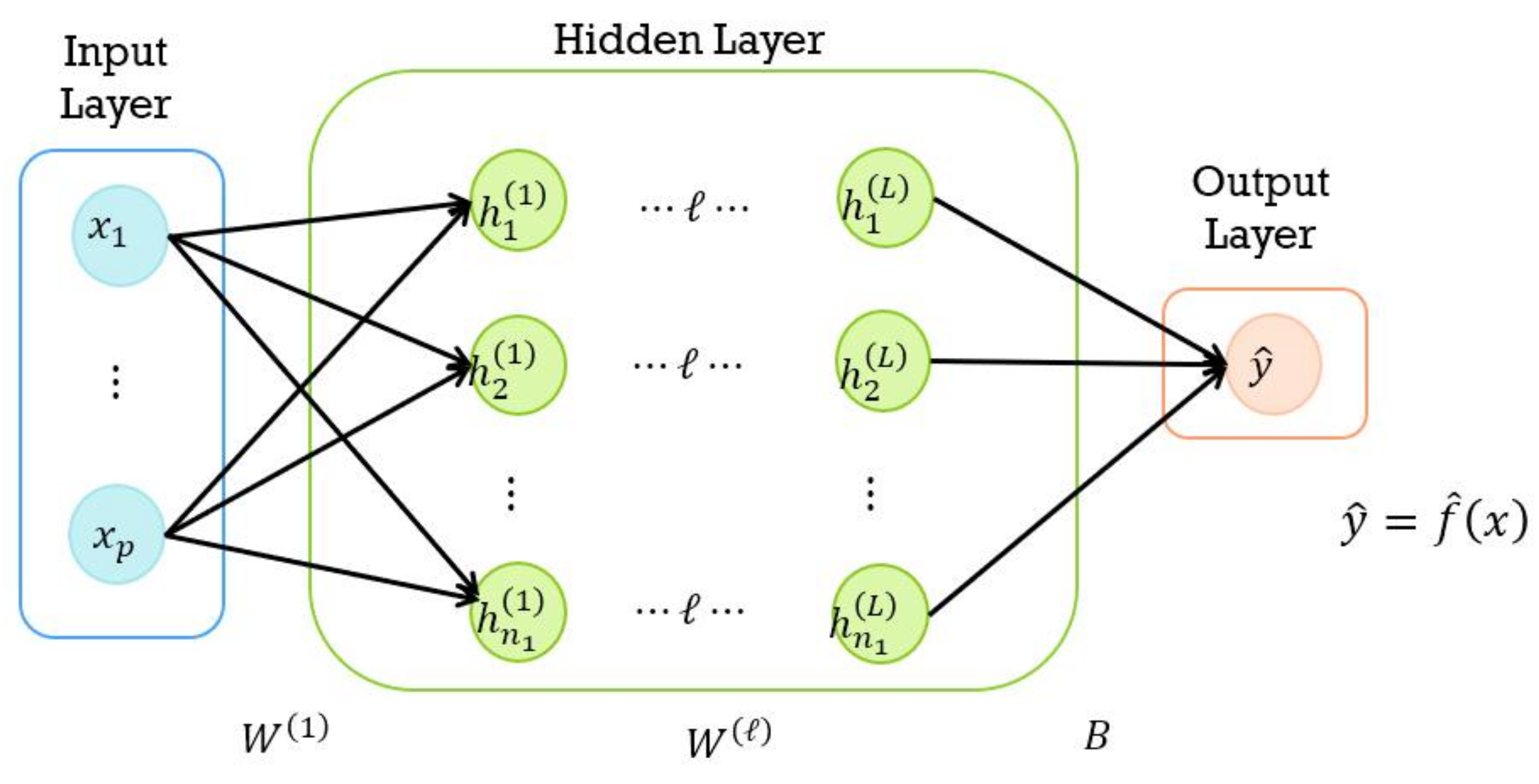
This section provides an overview of the fundamental DNN framework followed by the introduction of the proposed DNN–OHE survival models.

4.1. DNN Model

The DNN models are structured neural networks that include input, hidden, and output layers representing and modeling the nonlinear relationship between the input and output variables [19,20]. The primary objective is to find a nonlinear predictor for the output variable y given input variables x.

In a given dataset $D=\{(y_i,{\mathit{x}}_i);i=1,\dots ,n\}$, $y_i$ is an output (or target) variable of the ith cluster and ${\mathit{x}}_i={(x_{i1},\dots ,x_{ip})}^T$ is the corresponding p-dimensional input (or feature) vector. Here, the $y_i$s are assumed to be independent. The general structure of the DNN consists of one input layer, ℓ hidden layers ($\mathcal{\ell }=1,2,\dots ,L$), and one output layer, as shown in Figure 2. When the number of hidden layers is one it is called a neural network (NN), while when the number of hidden layers is two or more it is called a DNN. Here, $p_{\mathcal{\ell }}$ is the number of nodes in the ℓth hidden layer, $p_0=p$ is the number of nodes in the input layer, $W^{\left(\mathcal{\ell }\right)}=(w_0^{\left(\mathcal{\ell }\right)},w_1^{\left(\mathcal{\ell }\right)},\dots ,w_{p_{\mathcal{\ell }-1}}^{\left(\mathcal{\ell }\right)})$ is the weight matrix of the ℓ-hidden layer, and ${\mathit{w}}_i^{\left(\mathcal{\ell }\right)}=(w_{i1}^{\left(\mathcal{\ell }\right)},w_{i2}^{\left(\mathcal{\ell }\right)},\dots ,W_{i{p}_{\mathcal{\ell }}}^{\left(\mathcal{\ell }\right)})$ is the component vector of the ith node with element $w_{ij}^{\left(\mathcal{\ell }\right)}$, which is the jth weight of the ith node for each ℓ hidden layer. Here, $w_0^{\left(\mathcal{\ell }\right)}$ is the bias (intercept) vector of the $p_{\mathcal{\ell }}$ node of the ℓ hidden layer and $B={({\beta }_0,{\beta }_1,\dots ,{\beta }_{p_L})}^T$ is the weight vector of output layer, including the bias ${\beta }_0$. Now, the three layers (input, hidden, and output) constituting the DNN can be expressed as follows:

• Input layer:

  $$h_i^{\left(0\right)}=x_i(i=1,2,\dots ,p_0);$$
• Hidden layer:

  $$\begin{array}{ccc}\hfill h_j^{\left(1\right)}& =& \hfill f^{\left(1\right)}(\sum _{i=1}^{p_0}{w}_{ij}^{\left(1\right)}{h}_i^{\left(0\right)}+w_{0j}^{\left(1\right)}),j=1,\dots ,p_1,\hfill \\ \hfill h_j^{\left(2\right)}& =& \hfill f^{\left(2\right)}(\sum _{i=1}^{p_1}{w}_{ij}^{\left(2\right)}{h}_i^{\left(1\right)}+w_{0j}^{\left(2\right)}),j=1,\dots ,p_2,\hfill \\ & ⋮\\ & \\ \hfill h_j^{\left(L\right)}& =& \hfill f^{\left(L\right)}(\sum _{i=1}^{p_{L-1}}{w}_{ij}^{\left(L\right)}{h}_i^{(L-1)}+w_{0j}^{\left(L\right)}),j=1,\dots ,p_L;\hfill \end{array}$$
• Output layer:

  $$\widehat{y}=f^{\left(y\right)}(\sum _{j=1}^{p_L}{\beta }_j{h}_j^{\left(L\right)}+{\beta }_0)=f^{\left(y\right)}\left(NN\left(\mathit{x}\right)\right);$$

where $f^{\left(\mathcal{\ell }\right)}(·)$ and $f^{\left(y\right)}(·)$ are the activation functions of the ℓ hidden layer and output layer, respectively, and

$$NN\left(\mathit{x}\right)=NN(\mathit{x};\mathit{w},\mathit{\beta })=\sum _{j=1}^{p_L}{\beta }_j{h}_j^{\left(L\right)}+{\beta }_0$$

(5)

denotes a neural network (NN) predictor that describes a nonlinear function of $\mathit{x}$. Activation functions typically include linear, sigmoid, Tanh (hyperbolic tangent), and ReLU (rectified linear unit) functions. Specifically, a nonlinear function such as sigmoid or ReLU is commonly used as an activation function in the hidden layer, while the activation function in the output layer is selected as either a linear or nonlinear function depending on the type of output variables [20].

4.2. Learning Procedure of DNN

Next, we describe the learning procedure used to estimate the weights (i.e., model parameters) $\mathit{\theta }=(\mathit{w},\mathit{\beta })$ for the DNN in (5) using training data D. The estimation or learning process is conducted through the optimization of a loss function (called the objective function), which is denoted by $L\left(\mathit{\theta }\right)=L\left(f\right(\mathit{x}),y)$, which consists of true target y and true regression function $f\left(\mathit{x}\right)$, as in (1) and (2). It should be noted that a negative log-likelihood can be used as a loss function.

The model parameters $\mathit{\theta }$ are estimated by optimizing, that is, by minimizing the loss function $L\left(\mathit{\theta }\right)$; their estimates are defined by

$$\widehat{\mathit{\theta }}=\underset{\mathit{\theta }}{argmin}L\left(\mathit{\theta }\right),$$

and are equivalent to the maximum likelihood (ML) estimators of $\mathit{\theta }$, obtained by solving

$$\frac{\partial L\left(\mathit{\theta }\right)}{\partial \mathit{\theta }}=\mathbf{0}.$$

(6)

However, the estimating Equations (6) are generally complex and highly nonlinear. Therefore, gradient descent (GD) methods are often used to solve (6). For a given loss function L, the formula for updating parameters $\mathit{\theta }$ on iteration k using the GD method is provided by

$${\mathit{\theta }}_{k+1}={\mathit{\theta }}_k-\alpha \frac{\partial }{\partial {\mathit{\theta }}_k}L\left(\mathit{\theta }\right),$$

(7)

where $\alpha (>0)$ is the learning rate (or step size). Thus, for given initial values of $\mathit{\theta }$ and the learning rate $\alpha$, parameter estimation (or learning) is determined by computing the gradient vector $\partial L\left(\mathit{\theta }\right)/\partial {\mathit{\theta }}_k$ in (7), i.e., back-propagation [21]. It is important to note that optimization of $L\left(\mathit{\theta }\right)$ is usually performed using a mini-batch stochastic GD (SGD) method, particularly for very large datasets.

4.3. One-Hot Encoding (OHE)

The growth environment of individual tomato subjects may be similar within the same farm even if it is heterogeneous across different farms. This farm effect can be treated as a fixed effect, with the farm feature represented through the OHE method. OHE is a process in which categorical variables are converted into binary variables that take values of 0 or 1; it is sometimes known as dummy encoding. If there are multiple farms with several tomato plants, OHE creates binary variables (features) $z_1,\dots ,z_q$, where the element $z_{ki}$ equals one if tomato plant i belongs to farm k and equals 0 otherwise. Figure 3 illustrates the OHE method considering the farm index. Note that $q=65$ for the tomato data in Section 2.1.

4.4. DNN–OHE Survival Models

To consider the tomato farm effect as a fixed effect, we propose a DNN model based on OHE. The proposed models can be described by the following two types according to their method of applying OHE to the DNN model:

• DNN-I (DNN OHE-input): the DNN model applies OHE to the input layer (I).
• DNN-L (DNN OHE-last): the DNN model applies OHE to the last hidden layer (L).

Figure 4 presents a schematic representation of the DNN-I model, a DNN model in which the farm ID is applied to the input layer (I). This indicates that in the input layer the ID variables represented as OHE are combined with the 30 input variables from Table 1. DNN-I is a natural choice, as the binary variables generated by OHE continue to be treated as input variables. On the other hand, Figure 5 shows a schematic representation of the DNN-L model, in which the farm ID is applied to the last hidden layer (L), i.e., just before the output layer. This indicates that another input layer with only the ID variables is combined together with the last hidden layer in the output layer.

Accordingly, the two DNN–OHE models, namely, DNN-I and DNN-L, can be easily applied to the AFT model (1) and Cox model (2) to analyze the harvest time. The resulting models are described below. The DNN–OHE model based on the AFT model follows

$$T=f\left(\mathit{x}\right)+ϵ,$$

where $f\left(\mathit{x}\right)=NN(\mathit{x};\mathit{w},\mathit{\beta })$ is the NN predictor in (5). The DNN–OHE model based on the Cox model follows

$$\lambda \left(t\right|\mathit{x})={\lambda }_0\left(t\right)exp\left(f\left(\mathit{x}\right)\right),$$

where $f\left(\mathit{x}\right)=NN(\mathit{x};\mathit{w},\mathit{\beta })$ is the same NN predictor except without the bias ${\beta }_0$ in (5).

5. Prediction Performance Results of DNN Survival Models

5.1. Model Fitting and Predictive Measures

In this section, we aim to compare the predictive performance of the proposed DNN-I and DNN-L survival models with the existing AFT and Cox PH models and their corresponding DNN models. All DNN models, including the proposed models, were computed using Python-based TensorFlow-Keras, while the Cox PH model was implemented using the lifelines package in Python.

The total dataset was divided into three separate sets; within each farm, the last three observations were assigned to the test set, the middle four observations were assigned to the validation set, and the remaining observations were assigned to the training set.

The optimal hyperparameters used in the DNN models are summarized in

Table 3. Optimal hyperparameter settings.

Hyper Parameter	Setting
No. of hidden layers	3
No. of nodes per layer	$\{2,32,16\}$
Learning rate	0.001
Batch size	length of validation set of y
No. of epoch	1000
Activation function (hidden layer)	elu
Activation function (output layer)	linear
Optimizer (AFT-type models)	AdamW
Optimizer (Cox-type models)	Nadam

; early stopping was employed to prevent overfitting [20]. In the Cox model DNN, the negative Efron log-likelihood [22] was used as the loss function, while the RMSE loss was utilized in the AFT-based DNN because it penalizes larger errors more, especially when there is no censoring.

Note that $y_i=T_i$ in Section 4.1 due to no censoring. The predictive performance for survival models based on the $T_i$s without censoring was evaluated using the following measures. For the AFT-type models, we used the RMSE and mean absolute error (MAE), defined as follows:

$$\mathrm{RMSE}=\sqrt{\frac{1}{n}\sum _{i=1}^n{(T_i-{\widehat{T}}_i)}^2}$$

and

$$\mathrm{MAE}=\frac{1}{n}\sum _{i=1}^n|T_i-{\widehat{T}}_i|,$$

respectively, where $T_i$ is the ith observed harvest time and ${\widehat{T}}_i$ is the ith harvest time predicted by the fitted model. The MAE is more robust against outliers compared to the RMSE. Notably, AFT-type models are particularly useful for predicting the harvest time because they directly model the survival times.

For the Cox-type hazard models we used the concordance index (C-index), defined as

$$\begin{array}{ccc}\hfill C_H& =& P({\widehat{T}}_i<{\widehat{T}}_j|T_i<T_j)\hfill \\ & =& \hfill P(f\left({\mathit{x}}_i\right)>f\left({\mathit{x}}_j\right)|T_i<T_j);\hfill \end{array}$$

here, $f\left({\mathit{x}}_i\right)$ is the risk function of ${\mathit{x}}_i$ in (2), and is estimated as follows [23]:

$${\widehat{C}}_H=\frac{{\sum }_i{\sum }_j{\delta }_{i}I(T_i<T_j)\{I({\widehat{T}}_i<{\widehat{T}}_j)+0.5I({\widehat{T}}_i={\widehat{T}}_j)\}}{{\sum }_i{\sum }_j{\delta }_{i}I(T_i<T_j))}$$

where ${\delta }_i$ is the censoring indicator of the ith observation and ${\widehat{T}}_i$ is the ith observed harvest time, which is the corresponding predicted harvest time obtained from the fitted model. The C-index takes a value between 0 and 1, with values closer to 1 indicating better predictive performance. Note that Cox-type models are particularly useful for predicting survival probability, i.e., the survival function; the survival probability can be easily computed using the Cox hazard model, as shown in (3) and (4). We used the time-dependent Brier Score (BS) to evaluate the accuracy of the predicted survival function at a given time point t. The BS represents the average squared distance between the observed survival status and the predicted survival probability at that time point t, and is defined by for a given time point t as follows:

$$BS\left(t\right)=E{\{I(T>t)-S\left(t\right|\mathit{x})\}}^2.$$

Without censoring, the BS is estimated as follows [24]:

$$\widehat{B}S\left(t\right)=\frac{1}{n}\sum _{i=1}^n{\{I(T_i>t)-\widehat{S}\left(t\right|{\mathit{x}}_i)\}}^2,$$

where $\widehat{S}\left(t\right|{\mathit{x}}_i)$ represents the predicted survival function obtained from the fitted model. Note that a lower BS indicates better prediction performance, similar to the RMSE. The integrated BS (IBS) provides an overall evaluation of model performance across all available times ($t_1<t<t_{\max }$). The IBS over the interval $[0,t_{\max }]$ for $t_1=0$ is defined as

$$IBS=\frac{1}{t_{\max }}{\int }_0^{t_{\max }}BS\left(s\right)ds.$$

5.2. Prediction Results for AFT-Type DNN Models

We first consider the four AFT-type models: AFT, AFT-DNN, AFT-DNN-I, and AFT-DNN-L. Figure 6 illustrates the predicted values of T against the observed values of T on the test set. The results suggest that the AFT DNN-L model effectively predicts the output variables, with a Pearson’s sample correlation coefficient of 0.624. Furthermore,

Table 4. RMSE and MAE results of the four AFT-type models on the tomato data test set.

Predictive Measure	AFT	AFT-DNN	AFT-DNN-I	AFT-DNN-L
RMSE	0.8257	0.8124	0.9726	0.8067
MAE	0.6487	0.6167	0.7375	0.6090

demonstrates that the AFT DNN-L model achieves the lowest RMSE (0.8067) and MAE (0.6090), indicating superior performance.

Table 4 compares the prediction performances of the AFT-type methods with those of three popular machine learning (ML) methods: random forest (RF; [25]), XGBoost (XGB; [26]), and support vector regression (SVR; [27]). The hyperparameters for the three ML methods were tuned using ten-fold cross-validation through the Python packages RandomForestRegressor, xgboost, and svm, and the resulting optimal settings were as follows: (i) for the RF model, the number of trees was 500, the number of features randomly selected as candidates for splitting a node was $\sqrt{p}$, and the maximum depth of trees was ten; (ii) for the XGB model, the number of trees was 300, the learning rate was 0.1, and the maximum depth of trees was one; (iii) for the SVR model, the trade-off between maximizing the margin and minimizing the error was 0.1, the width of the margin was 0.01, and the kernel function was linear. The resulting ML predictive results are summarized as follows: for RF, the RMSE was 1.1929 and the MAE was 0.9384; for XGB, the RMSE was 1.2256 and the MAE was 0.9443; and for SVR, the RMSE was 1.1973 and the MAE was 0.9314. It is worth noting that none of these three ML methods are able to directly account for the farm effect. Consequently, we observe that all three ML methods yield inferior predictive results compared to the AFT–DNN methods presented in Table 4.

5.3. Prediction Results for Cox-Type DNN Hazard Models

Next, we consider the four Cox-type hazard models: Cox, Cox-DNN, Cox-DNN-I, and Cox-DNN-L.

Table 5. C-index and IBS results of four Cox-type hazard models on the tomato data test set.

Predictive Measure	Cox	Cox-DNN	Cox-DNN-I	Cox-DNN-L
C-index	0.6582	0.6527	0.6506	0.6600
IBS	0.1125	0.0471	0.0584	0.0468

presents the C-index and IBS results for the four Cox-type models on the test set. Among these models, the Cox-DNN-L model demonstrates the highest performance in terms of the C-index and IBS. Figure 7 displays the time-dependent BS results on the test set for the four Cox-type models. The BS values of the proposed Cox-DNN-L model and Cox-DNN model are very similar at each time point (week), and are consistently lower than those of the other two models (Cox and Cox-DNN-I) across almost all time points. Notably, the base Cox model exhibits exceptionally high BS values for weeks 6 and 8. These results indicate that the proposed Cox-DNN-L model outperforms the other three Cox-type models (Cox, Cox-DNN, and Cox-DNN-F) in terms of overall prediction performance.

6. Discussion and Conclusions

In this paper, we have presented DNN modelling approaches for tomato plants that take into account the farm effect. Because each farm has multiple tomato plant subjects, outcomes within the same farm can be correlated. Through analysis of the tomato data in Table 4 and Table 5, we observe that the proposed DNN survival models (AFT-DNN-L and Cox-DNN-L) demonstrate the best model performance in terms of predictive measures (RMSE, MAE, C-index, and IBS) for both harvest time and hazard rate as compared to the existing AFT-type and Cox-type models. In particular, we find that the three machine learning methods (i.e., RF, XGB, and SVR) used for the AFT-type models show relatively poor performance compared to all the AFT–DNN methods in Table 4. These results confirm that taking the farm effect into consideration enhances the models’ predictive capability.

In conclusion, the proposed DNN–OHE models (DNN-I and DNN-L) can be easily implemented using the existing DNN modeling approach. However, we recommend using the DNN-L model when considering farm effects, as the DNN-I model can pose computational problems due to the large number of parameters in the neural network as the number of farms increases [4] and provided lower prediction performance compared to the DNN-L model on our tomato data. One advantage of the proposed DNN-L method is that it can predict harvest times for individual tomato farms. This can assist farmers in improving or modifying their strategies to optimize yields and quality while reducing labor and resource usage [28].

Because it incorporates the farm effect based on OHE, the proposed DNN-L model can be applied to various types of data from smart farms, including yield data, sequential data, and image data. Belouz et al. [29] used artificial neural networks for the prediction of tomato yields, while Cho et al. [5] studied an encoding attention-based long short-term memory (LSTM) network. Minagawa and Kim [3] demonstrated the prediction of harvest times using a mask region-based convolutional neural network (Mask R-CNN [30]) to detect tomato bunch images. Furthermore, Nugroho et al. [31] compared the prediction accuracy of models based on Faster R-CNN, multibox Single-Shot Detector (SSD), and You Only Look Once (YOLO) for detecting tomato ripeness using input images [32,33,34,35,36]. Developing a DNN-L framework that allows for the above deep learning methods would be an interesting task for future research.

Another potential avenue for future work is to develop a new deep learning survival model that treats the farm effect considered in this paper as a random effect.

References

1. Na, M.H.; Park, Y.; Cho, W.H. A study on optimal environmental factors of tomato using smart farm data. JKDISS 2008, 10, 1427–1435. [Google Scholar]
2. Gadekallu, T.R.; Rajput, D.S.; Reddy, M.P.K.; Lakshmanna, K.; Bhattacharya, S.; Singh, S.; Jolfaei, A.; Alazab, M. A novel PCA–whale optimization-based deep neural network model for classification of tomato plant diseases using GPU. J. Real-Time Image Process. 2021, 18, 1383–1396. [Google Scholar] [CrossRef]
3. Minagawa, D.; Kim, J. Prediction of harvest time of tomato using mask R-CNN. AgriEngineering 2022, 4, 356–366. [Google Scholar] [CrossRef]
4. Hancock, J.T.; Khoshgoftaar, T.M. Survey on categorical data for neural networks. J. Big Data 2020, 7, 28. [Google Scholar] [CrossRef]
5. Cho, W.; Kim, S.; Na, M.; Na, I. Forecasting of tomato yields using attention-based LSTM network and ARMA Model. Electronics 2021, 10, 1576. [Google Scholar] [CrossRef]
6. Kim, J.C.; Kwon, S.; Ha, I.D.; Na, M.H. Survival analysis for tomato big data in smart farming. JKDISS 2021, 32, 361–374. [Google Scholar] [CrossRef]
7. Kim, J.C.; Kwon, S.; Ha, I.D.; Na, M.H. Prediction of smart farm tomato harvest time: Comparison of machine learning and deep learning approaches. JKDISS 2022, 33, 283–298. [Google Scholar] [CrossRef]
8. Luna, R.; Dadios, E.; Bandala, A.; Vicerra, R. Tomato growth stage monitoring for smart farm using deep transfer learning with machine learning-based maturity grading. Agrivita 2020, 42, 24–36. [Google Scholar]
9. Haggag, M.; Abdelhay, S.; Mecheter, A.; Gowid, S.; Musharavati, F.; Ghani, S. An intelligent hybrid experimental-based deep learning algorithm for tomato-sorting controllers. IEEE Access 2019, 7, 106890–106898. [Google Scholar] [CrossRef]
10. Alajrami, A.; Abu-Naser, S. Type of tomato classification using deep learning. IJAPR 2019, 12, 21–25. [Google Scholar]
11. Grimberg, R.; Teitel, M.; Ozer, S.; Levi, A.; Levy, A. Estimation of greenhouse tomato foliage temperature using DNN and ML models. Agriculture 2022, 12, 1034. [Google Scholar] [CrossRef]
12. Jeong, S.; Jeong, S.; Bong, J. Detection of tomato leaf miner using deep neural network. Sensors 2022, 22, 9959. [Google Scholar] [CrossRef] [PubMed]
13. Lawless, J.F. Statistical Models and Methods for Lifetime Data, 2nd ed.; Wiley: New York, NY, USA, 2003. [Google Scholar]
14. Ha, I.D.; Jeong, J.H.; Lee, Y. Statistical Modelling of Survival Data with Random Effects: H-Likelihood Approach; Springer: Singapore, 2017. [Google Scholar]
15. Kalbfleisch, J.D.; Prentice, R.L. The Statistical Analysis of Failure Time Data; Wiley: New York, NY, USA, 1980. [Google Scholar]
16. Kumar, U.A. Comparison of neural networks and regression analysis: A new insight. Expert Syst. Appl. 2005, 29, 424–430. [Google Scholar] [CrossRef]
17. Cox, D.R. Regression models and life tables (with Discussion). J. R. Stat. Soc. B 1972, 74, 187–220. [Google Scholar]
18. Breslow, N.E. Covariance analysis of censored survival data. Biometrics 1974, 30, 89–99. [Google Scholar] [CrossRef] [PubMed]
19. LeCun, Y.; Bengio, Y.; Hinton, G. Deep learning. Nature 2015, 521, 436–444. [Google Scholar] [CrossRef] [PubMed]
20. Goodfellow, I.; Bengio, Y.; Courville, A. Deep Learning; MIT Press: Cambridge, MA, USA, 2016. [Google Scholar]
21. Rumelhart, D.E.; Hinton, G.E.; Williams, R.J. Learning representations by back-propagating errors. Nature 1986, 323, 533–536. [Google Scholar] [CrossRef]
22. Sun, T.; Wei, Y.; Chen, W.; Ding, Y. Genome-wide association study-based deep learning for survival prediction. Stat. Med. 2020, 39, 4605–4620. [Google Scholar] [CrossRef]
23. Harrell, F.E.; Lee, K.L.; Mark, D.B. Multivariable prognostic models: Issues in developing models, evaluating assumptions and adequacy, and measuring and reducing errors. Stat. Med. 1996, 15, 361–387. [Google Scholar] [CrossRef]
24. Graf, E.; Schmoor, C.; Sauerbrei, W.; Schumacher, M. Assessment and comparison of prognostic classification schemes for survival data. Stat. Med. 1999, 18, 2529–2545. [Google Scholar] [CrossRef]
25. Breiman, L. Random forests. Mach. Learn. 2001, 45, 5–32. [Google Scholar] [CrossRef]
26. Chen, T.; Guestrin, C. XGBoost: A scalable tree boosting system. In Proceedings of the 22nd ACM SIGKDD International Conference on Knowledge Discovery and Data Mining, San Francisco, CA, USA, 13–17 August 2016; pp. 785–794. [Google Scholar]
27. Vapnik, V.; Golowich, S.E.; Smola, A.J. Support vector method for function approximation, regression estimation, and signal processing. Adv. Neural Inf. Process. Syst. 1997, 9, 281–287. [Google Scholar]
28. Liu, S.-C.; Jian, Q.-Y.; Wen, H.-Y.; Chung, C.-H. A crop harvest time prediction model for better sustainability, integrating feature selection and artificial intelligence methods. Sustainability 2022, 14, 14101. [Google Scholar] [CrossRef]
29. Belouz, K.; Nourani, A.; Zereg, S.; Bencheikh, A. Prediction of greenhouse tomato yield using artificial neural networks combined with sensitivity analysis. Sci. Hortic. 2022, 293, 110666. [Google Scholar] [CrossRef]
30. He, K.; Gkioxari, G.; Dollár, P.; Girshick, R. Mask R-CNN. IEEE Int. Conf. Comput. Vis. 2017, 322, 2980–2988. [Google Scholar]
31. Nugroho, D.P.; Widiyanto, S.; Wardani, D.T. Comparison of deep learning-based object classification methods for detecting tomato ripeness. Int. J. Fuzzy Log. Intell. 2022, 22, 223–232. [Google Scholar] [CrossRef]
32. Afonso, M.; Fonteijn, H.; Fiorentin, F.S.; Lensink, D.; Mooij, M.; Faber, N.; Polder, G.; Wehrens, R. Tomato fruit detection and counting in greenhouses using deep learning. Front. Plant Sci. 2020, 11, 571299. [Google Scholar] [CrossRef] [PubMed]
33. Mishra1, A.M.; Harnal1, S.; Gautam, V.; Tiwari, R.; Upadhyay, S. Weed density estimation in soya bean crop using deep convolutional neural networks in smart agriculture. J. Plant Dis. Prot. 2022, 129, 593–604. [Google Scholar] [CrossRef]
34. Kaur, P.; Harnal, S.; Tiwari, R.; Upadhyay, S.; Bhatia, S.; Mashat, A.; Alabdali, A.M. Recognition of leaf disease using hybrid convolutional neural network by applying feature reduction. Sensors 2022, 22, 575. [Google Scholar] [CrossRef]
35. Ireri, D.; Belal, E.; Okinda, C.; Makange, N.; Ji, C. A computer vision system for defect discrimination and grading in tomatoes using machine learning and image processing. Artif. Intell. Agric. 2019, 2, 28–37. [Google Scholar] [CrossRef]
36. Arthur, Z.; Hugo, E.; Juliana, A. Computer vision based detection of external defects on tomatoes using deep learning. Biosyst. Eng. 2020, 190, 131–144. [Google Scholar]
Figure 1. Histograms of the transformation of the harvest time [7].
Agriculture 13 01782 g001
Figure 2. A schematic diagram of a deep neural network; bias terms are omitted for brevity, and can be found in the main text.
Agriculture 13 01782 g002
Figure 3. A schematic diagram of one-hot encoding (OHE) for the farm index.
Agriculture 13 01782 g003
Figure 4. Schematic diagram of the DNN–OHE-input model (DNN-I).
Agriculture 13 01782 g004
Figure 5. Schematic diagram of the DNN–OHE-last model (DNN-L).
Agriculture 13 01782 g005
Figure 6. Predicted value of T against observed value of T and correlation (corr) results of the four AFT-type models on the tomato data test set.
Agriculture 13 01782 g006
Figure 7. Time-dependent Brier scores for four Cox-type hazard models on the tomato data test set.
Agriculture 13 01782 g007