Abstract
Arable land loss has become a critical issue in China because of rapid urbanization, industrial expansion, and unsustainable agricultural practices. While previous studies have explored the factors contributing to this loss, they often fall short in addressing the challenges of spatial heterogeneity and large-scale dataset analysis. This research introduces an innovative approach to geographically weighted regression (GWR) for assessing arable land loss in China, effectively addressing these challenges. Focusing on Chongqing, Guizhou, and Yunnan Provinces over the past two decades, it examines spatial autocorrelation with R-squared values exceeding 0.6 and residuals. Eight factors, including environmental elements (rain, evaporation, slope, digital elevation model) and human activities (distance to city, distance to roads, population, GDP), were analyzed. By visualizing and analyzing R² spatial patterns, the results reveal a clear spatial agglomeration distribution, primarily in urban areas with industries, highly urbanized cities, and flat terrains near rivers, influenced by GDP, population, rain, and slope. The novelty of this study is that it significantly enhances GWR computational capabilities for handling extensive datasets by utilizing Compute Unified Device Architecture (CUDA) on a high-performance GPU cloud server. Simultaneously, it conducts comprehensive analyses of the GWR model’s local results through visualization and spatial autocorrelation tools, enhancing the interpretability of the GWR model. Through spatial clustering analysis of local results, this study enables targeted exploration of factors influencing arable land changes in various temporal and spatial dimensions while also evaluating the reliability of the model results.
1. Introduction
The presence of arable land is of utmost importance in various aspects such as food production, mitigation of climate change, preservation of biodiversity, and management of water resources [1]. The inclusion of this component within the global carbon cycle is of utmost importance [2,3]. The impact of alterations in both the quantity and quality of arable land on food production and food security is a significant concern [4]. China is globally recognized for its significant share of arable land, accounting for 7% of the total arable land available worldwide. Furthermore, it is noteworthy that China accommodates almost 20% of the global population [5]. This indicates that the per capita arable land quantity (1100 m2/person) falls significantly below the worldwide average (2300 m2/person) [6]. However, the few arable areas face significant challenges due to a multitude of causes. Between the years 2013 and 2022, there has been a consistent decline in China’s arable land, with an average annual drop of [7]. China, as the most populous nation globally, is confronted with the imminent challenge of food security because of the decline in its arable land area. Therefore, it is crucial to comprehend the evolutionary patterns in arable land and further investigate the factors contributing to the decline in arable land.
The transformation of arable land is intricately intertwined with human activities; therefore, numerous studies prioritize the investigation of rapid economic development, population growth, urbanization, agricultural reorganization, and other human-related factors as the primary drivers of arable land decline. For instance, Liu and Guo examined the correlation between economic growth and arable land conversion in China, utilizing a geographical panel regression model as their primary methodology. Their findings revealed a significant spatial interaction effect between these two variables [8]. In a separate study by Tu et al., urban expansion in 14 Chinese cities from 1980 to 2015 emerged as the predominant factor contributing to arable land depletion, accounting for 74.36% of the overall arable land loss [9]. Building upon this work, Tu et al. conducted further research and analysis, unveiling a relationship between arable–urban land conversion and economic determinants in China that followed an inverted U-shaped pattern [10]. Additionally, Alexander et al. identified population expansion as the primary driver of agricultural land use change, with shifts in dietary patterns also playing a crucial and escalating role [11]. Most current research has limitations due to their focus on anthropogenic variables, often lacking comprehensive comparative analysis across various parameters. However, it is essential to recognize the influence of environmental variables on arable land depletion, including changes in the natural environment resulting from climate change, soil erosion, geological disparities, and related phenomena [12,13]. Therefore, this study aims to investigate both the human and environmental variables contributing to arable land loss to elucidate the underlying mechanisms.
To investigate the relationship between driving factors and the loss of arable land, we employed the geographically weighted regression (GWR) model as our analytical framework. The GWR model considers the impact of geographic location changes on geographic elements and can overcome the limitations of global spatial regression models in explaining spatial heterogeneity, which facilitates the examination of regional disparities and spatial clustering phenomena. Many optimized GWR models have emerged recently. Mansour et al. utilized a multiscale geographically weighted regression (MGWR) model to explore the spatial differentials in the relationship between COVID-19 incidence rates and covariates in the Oman region. MGWR, compared with the GWR model, considered multiple spatial scales, using different weight functions at each scale, making it more suitable for datasets with complex spatial structures [14]. Tasyurek and Celik addressed the issue of spatial nonstationarity in datasets collected in meteorology, environmental management, and ecology by developing a new GWR technique (4D-GWR). The 4D-GWR model simultaneously considered and handled spatial (longitude, latitude), altitudinal, and temporal nonstationarities to enhance prediction accuracy [15]. Khalid and Zameer utilized the FastGWR model to assess real estate values in Lahore and Faisalabad, Pakistan. This model improved the computational speed of the GWR model by employing more efficient calculation strategies and technologies [16]. The derivation and optimization of GWR models allow for flexible adjustments according to specific study scenarios, providing more reliable model outputs for diverse research contexts.
However, the GWR model poses computational challenges, as it requires the development of an autoregressive model for each data point, leading to substantial processing time demands, especially when dealing with large and multidimensional datasets [17]. Consequently, the use of the GWR model in research has mainly focused on local and municipal analyses. For example, Liu et al. applied the GWR model to assess changes in land ecological security and its influencing factors in the Danjiangkou region [18]. Similarly, Yu et al. utilized the GWR model to investigate the impact of groundwater levels, rainfall, land use changes, and population density on land subsidence in the Beijing region [19]. Moreover, over the past decade, significant portions of arable land in China have undergone loss because of urbanization and policy implementations, such as the conversion of farmland into forested areas, among other contributing factors. Consequently, the examination of arable land loss typically requires a substantial volume of data, ranging from hundreds of thousands to even millions of data points. This has resulted in a scarcity of research at the provincial level regarding the utilization of the GWR model for the analysis of arable land loss.
To address the big data challenges faced by the GWR model, we propose leveraging GPU parallel computing technology to distribute computational tasks across multiple GPU computing nodes, facilitating collaborative computation [20]. The utilization of GPU parallel computing has been applied increasingly across various research domains. For instance, Tian, A. et al. employed the GWR-CUDA model to investigate spatial and temporal variations in wetlands across different scales in China and identify key factors contributing to wetland loss [21]. Wang et al. applied this model to analyze an extensive dataset of road curve accidents, aiming to uncover correlations between the frequency of road curve crashes and various characteristics [22]. Furthermore, Wang et al. introduced the FPGWR model (Fast-Parallel–GWR) based on CUDA. Verification using simulated datasets indicated that the runtime of FPGWR was negatively correlated with the number of CUDA cores, achieving computational efficiencies up to a thousandfold or even several tens of times [23]. Therefore, compared with traditional GWR methods, this algorithm substantially enhances computational efficiency and accuracy by capitalizing on the high-bandwidth memory capabilities of GPUs.
Currently, many studies predominantly rely on indicators such as adjusted R2, AICc values, etc., derived from the GWR model to explore the impact of various geographical factors on the dependent variable within different spatial contexts. However, the spatial distribution characteristics of GWR model results and the underlying reasons for such spatial distribution have been neglected in the existing literature. Tian, M. et al. employed the GWR model to examine geochemical data and explore the correlation between geochemical attributes and targets for mineral exploration. It utilized P-A diagrams to assess the relative importance of ore-forming elements (residues) and associated elements, indicating the location of the sought-after type of mineral deposits [24]. Li et al. primarily investigated the spatial distribution of crustaceans in coastal waters and their correlation with other environmental parameters by comparing various results such as AIC, R2, coefficient estimates, RMSE, etc., between GAM and GWR models [25]. It is evident that these studies focused on analyzing local results of the GWR model to explore the degree of influence of geographic factors on the dependent variable and the significance of the model while neglecting to provide a comprehensive explanation for the spatial characteristics of the local fitness outcomes and the underlying factors contributing to the variance in the distribution of GWR results. Exploring the spatial distribution of R2 contributes to the identification and understanding of spatial dependence in geographic spatial data [26]. Simultaneously, it helps unveil the heterogeneous structures present in geographic space, providing insights for a deeper understanding of the nature and patterns of geographic spatial data. The spatial clustering of R2 in the GWR model implies that the model possesses enhanced explanatory capabilities for the variability in geographic space [27]. It enables a more accurate reflection of the contributions of different geographic locations to the model, suggesting that certain regions may exhibit localized significance in terms of causal relationships or influential factors. Overall, the spatial clustering of R2 in the GWR model signifies a refined capacity to capture and explain the spatial nuances and localized impacts within the geographical context.
The novelty of this study is that it deployed the GWR-CUDA model on a GPU cloud server to handle large-scale data efficiently and analyzed the visualization of R2, residuals, and spatial autocorrelation compressively, which enhances the interpretability of the GWR model for explaining dynamic changes in arable land. Through spatial clustering analysis of local results, it enables targeted exploration of factors influencing arable land changes in different temporal and spatial dimensions, while also evaluating the reliability of the model results. Therefore, this research is significant because it provides a comprehensive understanding of the influencing factors in arable land changes and a thorough assessment of the interpretability and reliability of the model results. This can reveal the spatial heterogeneity and non-stationarity characteristics of the model. Section 3 of this paper provides a comprehensive overview of the study process, encompassing data gathering and processing, the development of the GWR-CUDA model environment, and the utilization of the GPU cloud server.
2. Study Area
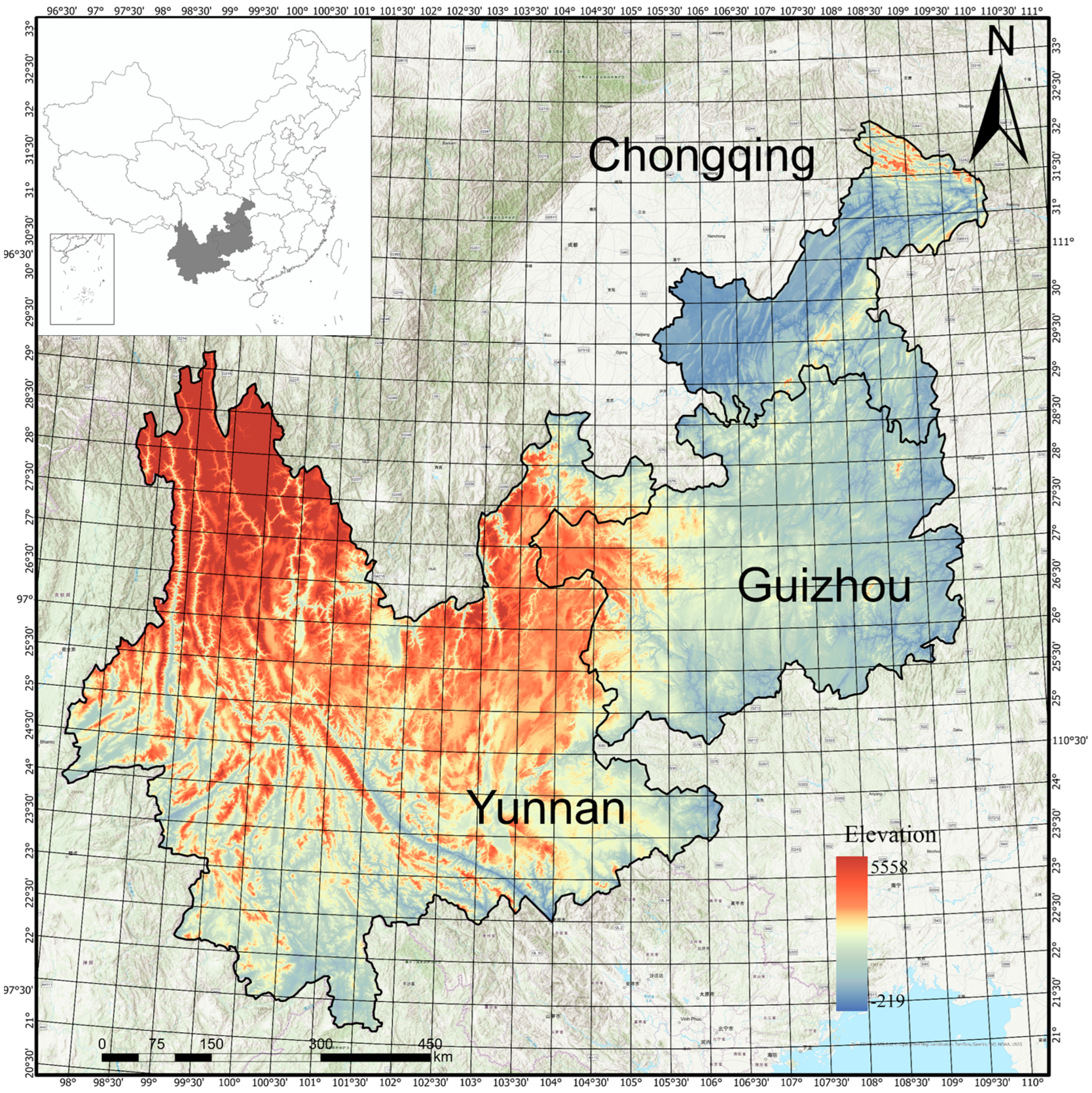
This study focuses on changes in arable land loss in the agricultural areas of southwest China, including Yunnan, Chongqing, and Guizhou Provinces (Figure 1). The region under consideration exhibits a wide range of environmental habitats and climatic conditions owing to its intricate topography (Table 1). This topography encompasses several geographical features, including the Kunming plateau, the karst landform in Guizhou Province, the mountainous areas and valleys along the Yangtze River, and the basin topography in Chongqing. This region has a humid subtropical climate and is subject to various influences caused by topography, which lead to great variation in annual precipitation and temperature (Table 1). Furthermore, recent data indicates that the proportion of arable land within each province amounts to approximately 20%. In recent years, heightened agricultural production, characterized by the escalated utilization of chemical fertilizers and pesticides, has resulted in soil erosion and contamination. The phenomenon of rapid urbanization and infrastructural development has given rise to alterations in land use patterns, leading to the loss of arable land and degradation of ecosystems. Yunnan, Guizhou, and Chongqing are strategically important regions for studying arable land loss because of their diverse geographical and socioeconomic characteristics. These provinces have varied topographies, including mountainous terrains, flat plains, and river valleys, which influence land use patterns. Additionally, they represent a mix of rapidly urbanizing regions (like Chongqing) and more rural, agriculturally reliant areas (like Yunnan and Guizhou). This diversity makes them excellent case studies for understanding the interaction between environmental factors (rain, evaporation, slope, DEM) and human activities (urbanization, economic development) in driving arable land loss.
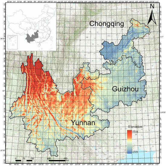
Figure 1.
Location of the study area—Chongqing, Guizhou, and Yunnan in China—and its elevation range.

Table 1.
Natural environmental information on the three provinces considered in this study.
3. Methods
3.1. Data Acquisition and Preprocessing
The dataset utilized in this study was categorized into two distinct categories as follows: socioeconomic data and environmental data. The socioeconomic data mostly comprised the population figures obtained from the CAS Data Center, along with the annual GDP data sourced from the website of the Institute of Geographical Sciences and Resources of the Chinese Academy of Sciences. The data spanned the years 2000 to 2020. The natural data utilized in this study encompassed raster land use data obtained from the Globe-Land30 dataset and the national roadmap data (https://geodata.pku.edu.cn/, accessed on 30 June 2024), slope, the digital elevation model (DEM), from which slope was calculated in ArcGIS, precipitation, and evaporation data. Table 2 presents the precise definitions and origins of the variables employed in this research. The data underwent resampling at a resolution of 30 m × 30 m. The spatial interpolation dataset covered the whole of China, in which the sample size related to the loss of arable land in the study area was about 340–350 w. During the preprocessing data stage, the data were normalized to have the same metric scale among features and eliminate outliers, and then the data with the non-zero loss rate of arable land were analyzed. Normalization is performed to eliminate scale differences among different features, enhancing the training effectiveness of a model. However, it does not reduce the dimensionality of the data; all geographic variable features are retained.
Table 2.
Abbreviated independent variables considered with their meanings and data sources.
Considering data accessibility and spatial resolution, the independent variable data were divided into human factors (population, GDP, distance to existing cities, and distance to major roads) and environmental factors (rain, evaporation, slope, and elevation in the form of DEM). When selecting the independent variables, all were considered to have a potential impact on the loss of arable land. For example, a smaller distance to the city means that the area of urban land will increase because of urban expansion, leading to a more significant loss of arable land [28].
3.2. GWR-CUDA
The GWR model was used in this study because of its potential to assess geographical heterogeneity by assigning various weights to each observation location [29]. In contrast to typical global regression models, the GWR model facilitates the creation of distinct regression connections for each geographical area, thereby capturing minor local differences [30,31]. This region-specific modeling approach permits a better understanding disclosure of hidden patterns within spatial data, giving finer and more precise analytical outcomes.
The GWR model equation can be expressed as
where , denotes the rate of arable land loss at location in the grid cell, denotes the values of the eight independent variables at location are the coordinates of regression analysis cell , and and are the intercept and regression coefficient, respectively.
Nevertheless, because of the GWR model’s increased computational complexity, a sizable amount of memory is required to handle the data used. Within research areas at the provincial scale, the raster pixels representing the extent of arable land loss amount to tens or hundreds of millions. Hence, it is not feasible to process these data points by the GWR model to generate the anticipated outcomes. To address challenges posed by big data effectively, a recommended approach involves partitioning the sequential computation of the GWR into parallel computations utilizing GPUs. To realize parallel computing of GWR, the fundamental concept involves the implementation of an interface that enables the simultaneous solution of numerous matrix inversions through the utilization of CUDA calls to NVIDIA Graphic Processing Units (GPUs), as proposed by Lu et al. [20]. CUDA is a general-purpose parallel computing architecture that enables high-performance computing operations on NVIDIA GPUs [32,33]. CUDA enables the utilization of GPUs for a diverse range of scientific computing, data processing, and machine learning tasks, expanding their functionality beyond the traditional domain of graphics rendering. In this study, the GWR model employed 64 CUDA cores for parallel computation, resulting in enhanced efficiency in model fitting.
In this study, we mainly implemented CUDA calls to GPUs through the GWmodel package in the R language, which enables parallel computation of the GWR model. In the R language environment under the CentOS 7 operating system, we introduced a dataset containing information on the loss rate of arable land, geographic influences, and geographic coordinates, and converted it into a geospatial data format. Then, we chose “bisquare” as the kernel function, CUDA as the parallel computation method, and the AICc criterion and adaptive approach to determine the most suitable bandwidth. After obtaining the optimal bandwidth, we performed a geographically weighted regression analysis. This method efficiently avoids memory overflow and reduces the runtime complexity of matrix operations. According to the experimental result, the maximum data volume (812,900) took about 20 h and 30 min for regression analysis by using single V100 GPU, and the minimum data volume (74,800) took only 9 min to process. To provide a more intuitive comparison, we evaluated the processing time of GWR4 (version: 4.09), a software tool for geographically weighted regression (GWR) analysis, against GWR-CUDA. For a data sample of 20,000 observations, GWR4 would have taken approximately 10 h to process, while GWR-CUDA only took 28 min, achieving a 21.5-fold reduction in time. In addition, four V100 high-performance graphics cards can simultaneously process four data partitions, reducing time costs.
3.3. Grid-Distributed Computing
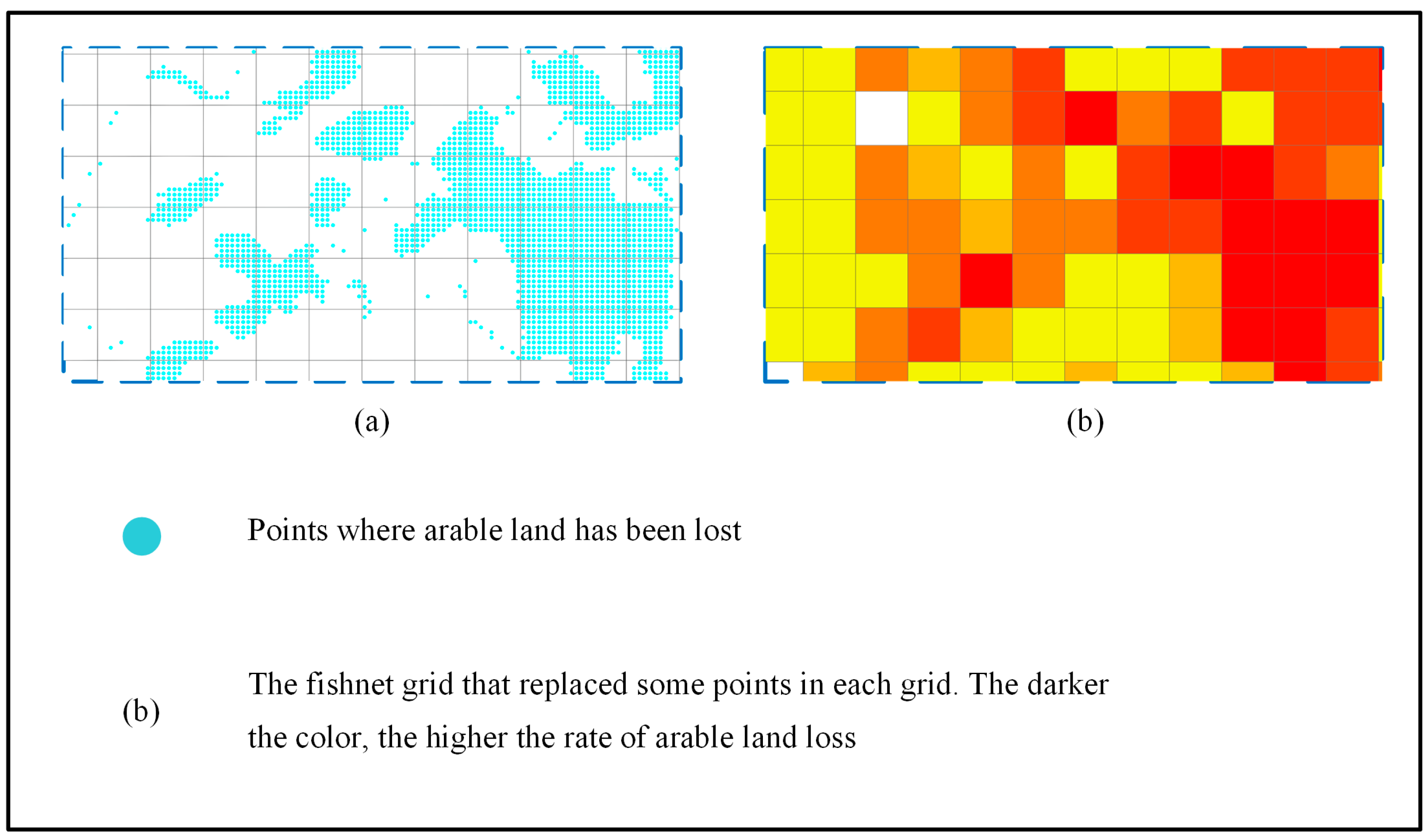
Building upon the GWR-CUDA model, we conducted data preprocessing by constructing a fishnet to distribute data points into different grid cells (as shown in Figure 2). A fishnet typically refers to a grid or raster used to divide maps or spatial data into uniform and regular regions for analysis, data management, and visualization purposes. This approach not only achieved a reduction in the volume of data processed by GWR but also transformed the arable land loss issue from a binary variable problem into a continuous variable problem that the GWR model can handle. In this context, data points with a value of 1 indicate arable land loss, while data points with a value of 0 indicate that it is still arable land. By creating a fishnet for data points, we calculated the arable land loss rate of the grid unit by dividing the sum of data points with the value of 1 (arable land loss occurred) by all data points (arable land loss occurred and retained as arable land). Then, we replaced the original data points with the loss rate as the target variable of the center point of the fishnet. Subsequently, we utilized the position-selecting tool to match the coordinates with the center points of the grid cell. Through this process, the attribute table of the fishnet encompassed the coordinate data and the dependent variable dataset.
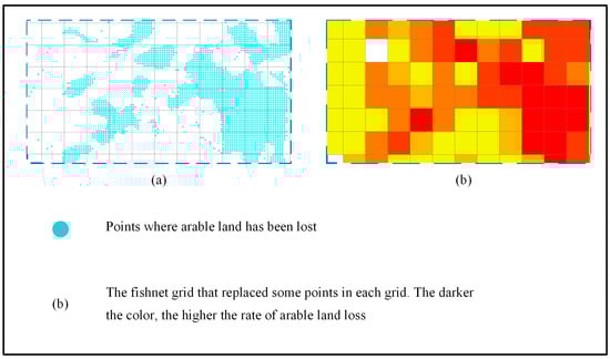
Figure 2.
The steps to implement GWR analysis with the grid method. (a) Create the fishnet, and (b) use the fishnet to demonstrate the arable land loss rate. The color of different degree represents the loss rate of arable land. The darker the color, the higher the rate of arable land loss.
The aforementioned approach can significantly decrease the amount of data by a factor of tens or even thousands in the southwestern region, particularly for places such as marshes and grasslands. Nevertheless, despite the possibility of reducing the data amount from tens of millions to a few million, processing such extensive data still requires assistance from conventional computer graphics cards. To address the data issue more effectively, we employed GPU cloud servers to enable GWR-CUDA distributed computing. This approach entailed utilizing a collection of 4*V100 multi-core high-performance graphics cards to process a given dataset collectively. The V100 graphics card, developed by NVIDIA, is a GPU designed for professional use. It has gained significant popularity in several domains such as high-performance computing and deep learning because of its ability to handle large-scale datasets efficiently [34]. Li et al. employed the V100 GPU for the purpose of preprocessing remote sensing photos and training a convolutional neural network in their recent investigation. The authors demonstrated that the utilization of V100 GPU resulted in notable enhancements in the training speed and efficiency of the convolutional neural network while maintaining classification accuracy, through a comparative analysis of training time and performance between CPU and V100 [35]. Therefore, the utilization of distributed computing on a cloud server that is equipped with many high-performance graphics cards significantly alleviates the computational burden on the GWR model, enabling the processing of extensive datasets obtained from cultivated fields. Additionally, to enhance computational efficiency and prevent memory overflow, we divided the provinces of Guizhou and Yunnan into three sections for the GWR-CUDA analysis. The data for arable land loss in both provinces amounted to around 1 million records. Given the high computational complexity of GWR, even with GPU processing, memory overflow can still occur. Therefore, we opted to partition the provinces into three sub-regions for more manageable analysis and processing.
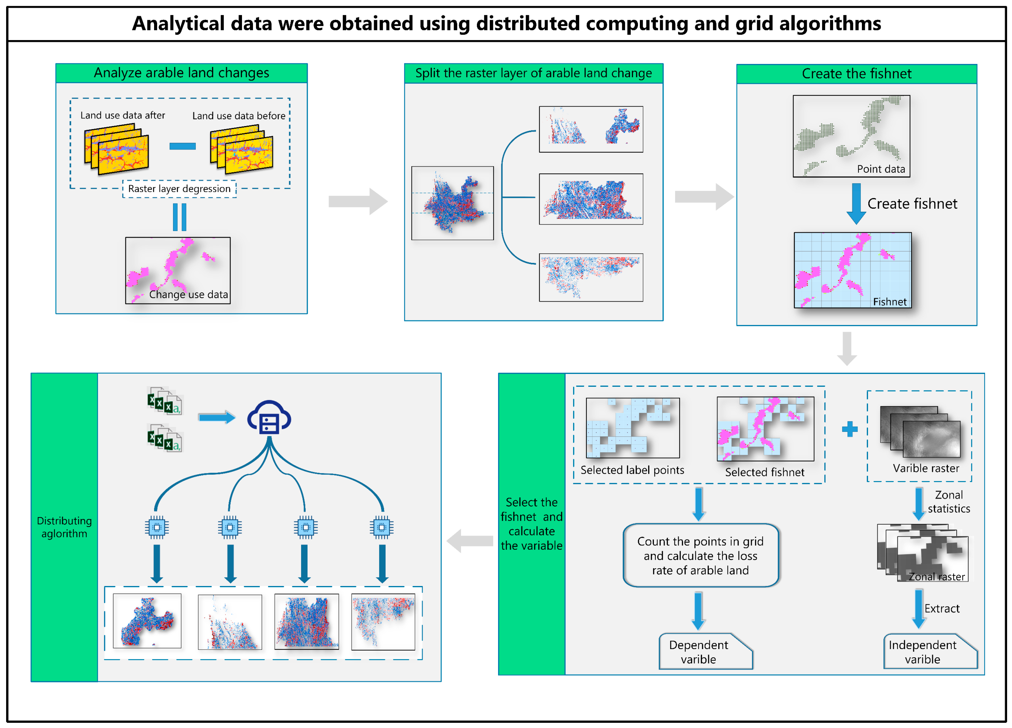
As shown in Figure 3, the main operational steps comprised the following seven steps to obtain the data required by the GWR model to study multiple drivers of arable land loss in the Yunnan, Chongqing, and Guizhou regions. (1) Obtain the arable land loss raster in the period using the raster images of two time points for subtraction. (2) Segment and extract the provinces into sub-regions. (3) Create a fishnet with 300 m × 300 m grid cells to cover the studied sub-regions and generate the corresponding point data and fishnet data. (4) Calculate the arable land loss rate within each grid cell and select the grid cell with arable land loss. (5) Use the filtered fishnet to perform partition statistics on the independent variable raster and calculate the mean value of the independent variable within each grid cell. (6) Extract independent and dependent variables from each raster cell, add latitude and longitude coordinates, and preprocess the independent variable to obtain the final data table required for the model. (7) Complete data analysis on the GPU cloud server to execute geographically weighted regression for each point.
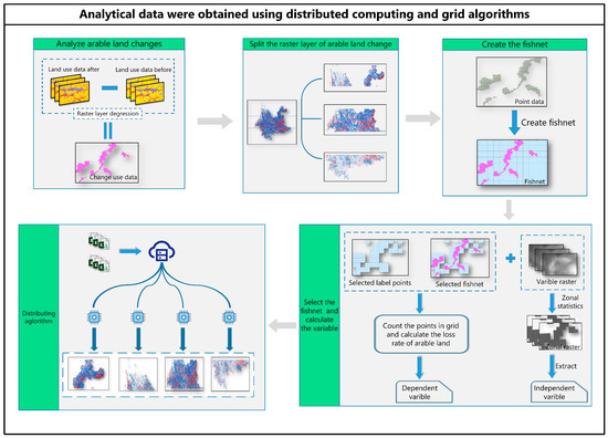
Figure 3.
Steps in the analysis of arable land loss rates using a fishnet.
3.4. Statistical Analysis of Spatial Results
Upon acquiring the outcomes of the GWR-CUDA model, we proceeded to evaluate the presence of a spatial aggregation trend in the high R2 values using Moran’s index. Moran’s index quantifies the spatial autocorrelation in a variable, specifically assessing the degree of similarity in attribute values among spatially neighboring regions. Spatial autocorrelation may manifest as positive or negative. An absolute value closer to 1 indicates a stronger spatial correlation. In this study, the spatial autocorrelation tool was used to calculate the correlation of the high adjusted R2 within the study area of Moran’s index. Values closer to 1 indicate stronger clustering, meaning similar values (either high or low) are spatially grouped together. Values closer to −1 indicate stronger dispersion, where similar values are spatially scattered, typically with high and low values alternating. Additionally, we employed visualization techniques to examine the adjusted R-squared, aiming to comprehend the distribution pattern of the spatial effect exerted by geographical elements on the loss of arable land [36]. The adjusted R2 is a refined coefficient of determination designed to evaluate the explanatory power of a regression model. Unlike the standard R2, the adjusted R2 accounts for the number of independent variables, mitigating the risk of overestimating model fit because of the inclusion of irrelevant predictors. A higher adjusted R2, approaching 1, indicates a superior fit of the GWR model, signifying that geographical factors robustly explain arable land loss. Conversely, a lower adjusted R2 implies weaker explanatory power. By analyzing the spatial distribution of R2, it is possible to reveal the main factors influencing arable land loss across different temporal and spatial scales, effectively reflecting the spatial heterogeneity and nonstationarity in geographical factors. This analysis helps to understand the complex spatial dynamics involved in the arable land loss process, providing a scientific basis for developing more targeted management and conservation strategies.
4. Results
4.1. Arable Land Loss in China between 2000 and 2020
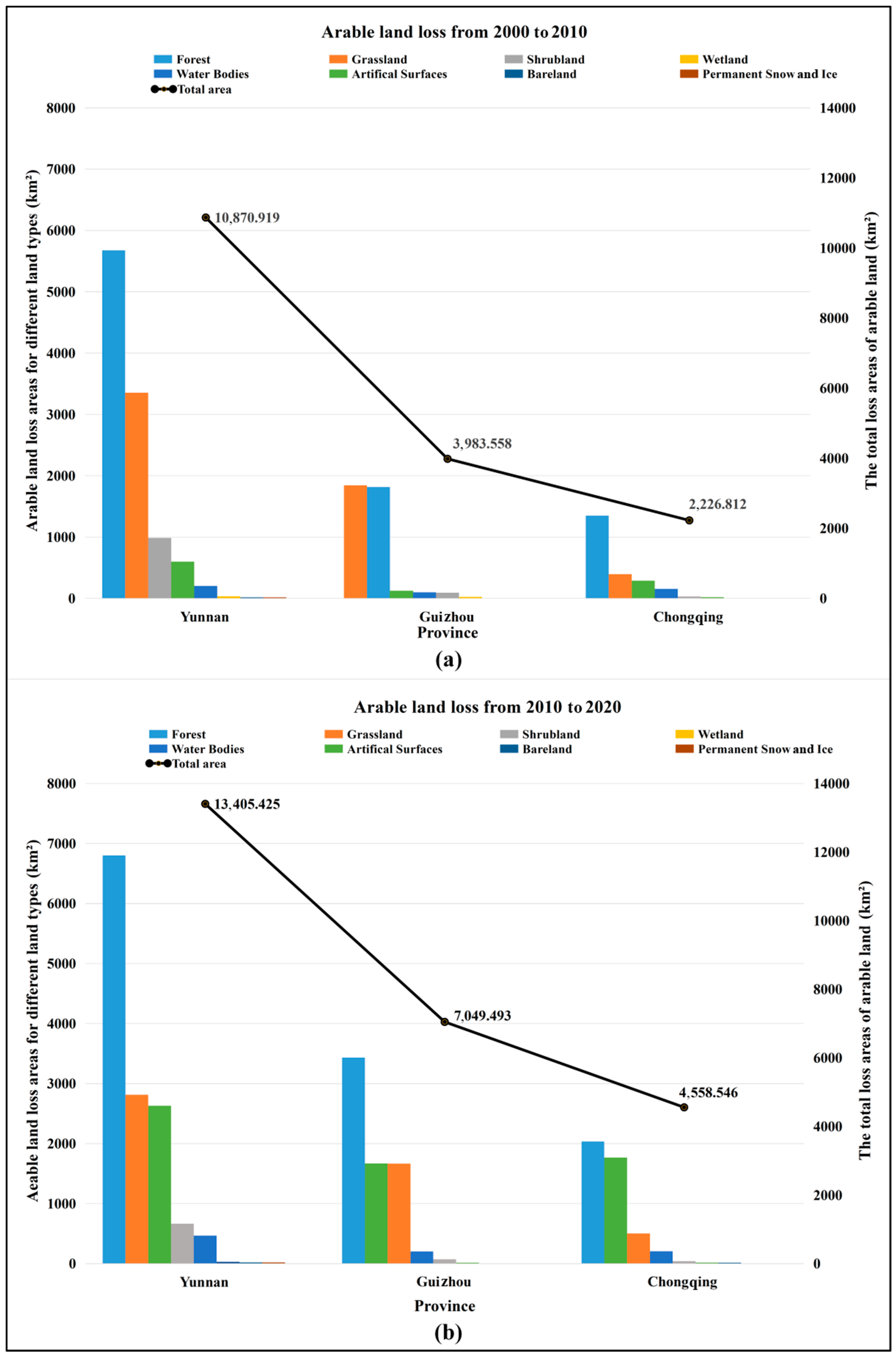
From 2000 to 2010, the total area of arable land lost in the region was 17,081.289. Among the three provinces, Yunnan had the largest area of loss, reaching 10,870.919, which accounted for approximately 64% of the total loss area in the three provinces (Figure 4a). However, the areas of loss in Chongqing and Guizhou were relatively small, accounting for only about 13% and 23%, respectively. The data presented in Figure 4b illustrates that from 2010 to 2020, the total area of arable land lost in the region was 25,013.464, which represented a 46.43% increase compared with the previous decade. This indicates that the situation of arable land loss in the region continuously deteriorated. Upon examining the situation in each province, it is evident that the loss of arable land deteriorated to varying degrees. Among them, Chongqing and Guizhou had a greater degree of deterioration, with increases of 104.71% and 76.94%, respectively. However, Yunnan Province still had the highest rate of arable land loss, with a total loss area of 13,405.425, which exceeded the combined loss area of arable land in Chongqing and Guizhou. From the perspective of where arable land was lost, forest and grassland are still the two most significant destinations for loss. However, unlike before, the area of arable land converted into artificial surfaces significantly increased, becoming another major destination of loss. This indicates that over the past decade, numerous human activities in the region led to the destruction of arable land. Furthermore, in Chongqing, there was a conversion of arable land to bare land.
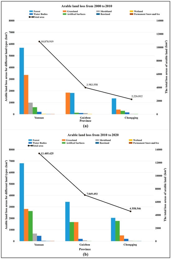
Figure 4.
Arable land loss during 2000–2010 (a) and 2010–2020 (b) in the three provinces considered in this study.
Figure 5 illustrates the overall trend in arable land changes in the study area. A comparison across different time periods reveals that although the general land use of arable land remained relatively stable, starting in 2010, the loss of arable land around major urban centers expanded significantly, leading to a gradual reduction in arable land area. For instance, in the southwestern urban core of Chongqing and the central–western region of Kunming in Yunnan Province, both the blank and red areas increased, indicating a reduction in arable land and an intensifying loss and loss of arable land around urban areas. In contrast, the changes in Guizhou Province were more dispersed. While the total amount of arable land remained relatively stable, the significant expansion of red areas suggests that arable land loss worsened, and substantial changes occurred in certain regions. Furthermore, the blue areas, representing an increase in arable land, showed little spatial variation between the two periods, remaining primarily in densely populated, flat regions. This indicates that the spatial pattern of arable land in these areas remained relatively stable.
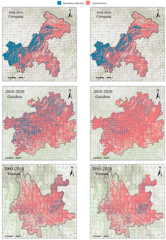
Figure 5.
Fishnet grid with arable land loss rates during 2000–2010 and 2010–2020.
4.2. Statistics of the Model Results
To analyze the data between 2000 and 2010, 2,586,334 equations were created throughout the fitting procedure for the entirety of the region. Among the equations considered, Yunnan accounted for a significant proportion of 1,471,904, representing 56.91% of the overall count. In contrast, Chongqing and Guizhou contributed 13.82% and 29.27% of the equations, respectively. To analyze the data between the years 2010 and 2020, a cumulative count of 2,954,311 equations was produced, with each province maintaining a comparable share relative to the preceding decade. As depicted in Table 3, upon examining the analysis outcomes of the three provinces in various time intervals, it became evident that the R2 values of the equations derived from the GWR-CUDA analysis predominantly fell within the 0.2–0.4 range. This range encompassed around 40% of the aggregate number of equations within each province.
Table 3.
Number of equations in different R2 value ranges after GWR-CUDA model fitting.
4.3. Spatial Distribution and Visualization of the GWR-CUDA Results
4.3.1. Spatial Distribution and Visualization of High R-Squared Values
The coefficient of determination, denoted as R2, is frequently employed as a measure to assess the adequacy of a regression model’s fit. A higher R2 value signifies a stronger degree of fit, whereas a lower R2 value not only indicates a weaker fit but also implies the possibility of a more intricate relationship between the dependent variable and the independent variables within the given region. Additionally, it suggests the potential involvement of other unaccounted factors or a weak association between the dependent variable and the chosen independent variables [37]. This study examined the significance of R2 values exceeding 0.6 as an indicator of a strong R2. These values were utilized to evaluate the model’s fitting performance and to conduct a comprehensive analysis of the factors contributing to arable land loss. By visualizing the fitting results, we discerned the presence of spatial non-smoothness, facilitating a more complete and in-depth comprehension of the factors contributing to the decline in arable land in various geographical areas.
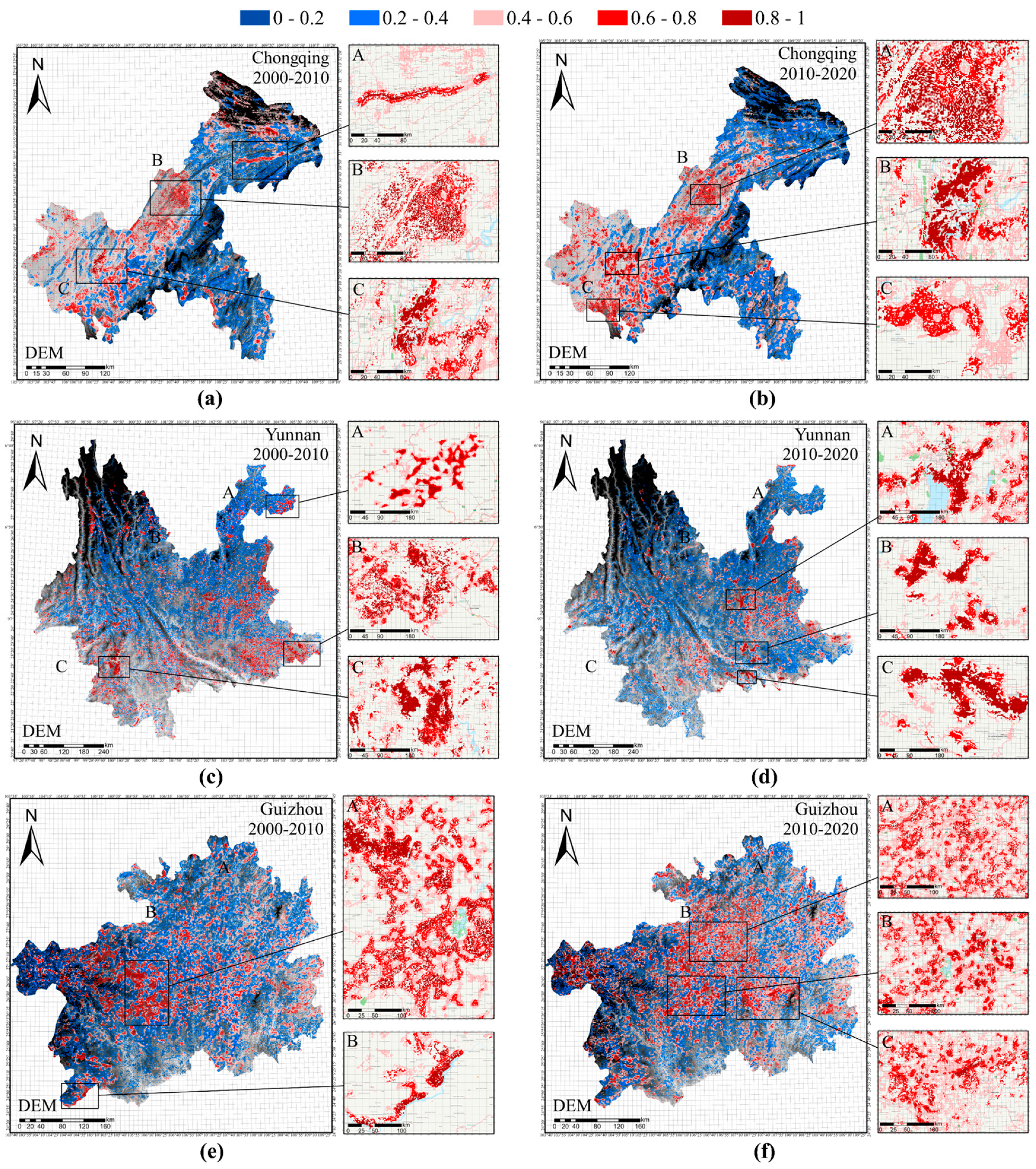
During the period of 2000–2010, the grids with high R2 in the Chongqing region were mainly agglomerated in the Yangtze River shoreline area from Yunyang County to Fengjie County, which is located in the ecological and economic zone of the Three Gorges Reservoir Area (Figure 6a(A)). Furthermore, they were also agglomerated in the north of Zhong County, which is also situated in the heart of the Three Gorges Reservoir Area, as well as in the surrounding areas of the primary urban center of Chongqing, such as Yubei, Jiangbei, and Shapingba District (Figure 6a(B,C)). In Yunnan, the agglomeration mainly occurred in Zhenxiong County, which is located at the junction of Yunnan, Guizhou, and Sichuan Provinces (Figure 6b(A)). Additionally, Napo County in the southeast and the eastern region of Pu’er City along the Lancang River also experience agglomeration (Figure 6b(B,C)). However, the agglomerating phenomenon in Guizhou Province was not as significant as in the previous two provinces. Its distribution mainly displayed an alternating pattern with high and low R2 values. Among them, there were two main locations where the agglomerating was more apparent—the junction of Guiyang City and Zhijin County (Figure 6c(A)), and Wanfeng Lake, which is located at the boundary of Guizhou, Guangxi, and Yunnan provinces (Figure 6c(B)).
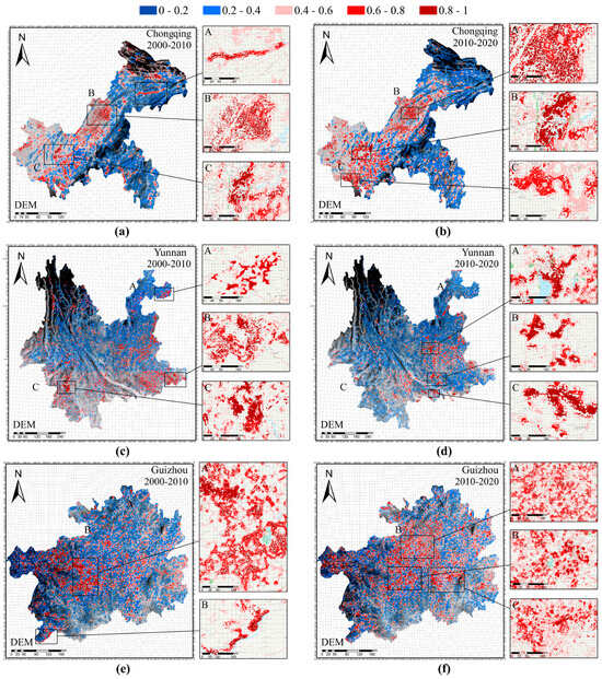
Figure 6.
Spatial distribution of R2 during 2000–2010 and 2010–2020 in the three provinces considered in this study. The color gradient represents the distribution of adjusted R2 values across intervals. Deeper colors signify higher R2 values, indicating stronger explanatory power of the variables for farmland degradation, while lighter colors indicate lower R2 values, reflecting weaker explanatory power. The subgraph represents the highly adjusted R2 cluster area.
From 2010 to 2020, the phenomenon of spatial agglomeration became more prominent. There were no significant changes in the location of agglomeration in Chongqing, except for the exclusion of Yunyang County and the inclusion of the area of Jiangjin District that borders Sichuan Province (Figure 6d(C)), while the main urban area presented a more striking agglomerating phenomenon around Yuzhong District (Figure 6d(B)). In Yunnan and Guizhou, on the other hand, the locations of the agglomerations changed to varying degrees. Yunnan underwent considerable changes, with its agglomerating locations now located in the middle and south of Kunming and Honghe Hani and Yi Autonomous Prefecture (Figure 6e). In contrast, the change in Guizhou was relatively slight, and its spatial distribution was still scattered, but its agglomeration phenomenon strengthened compared with the previous one, which was mainly concentrated in the surrounding cities centered on Guiyang, such as the southern part of Zunyi (Figure 6f(A)), Qianxi City (Figure 6f(B)), and Qiandongnan Miao and Dong Autonomous Prefecture (Figure 6f(C)).
Afterward, we utilized spatial autocorrelation tools to verify the spatial clustering phenomenon of R2. The results revealed that the Moran’s I indices for each province during the two periods were positive, ranging from 0.78 to 0.97, and the corresponding z-scores all exceeded 1.96. This indicates a significant positive spatial correlation in R2 in different regions of the three provinces, implying a pronounced spatial clustering of R2 values across space [38]. Specific indicators are detailed in Table 4. The spatial clustering of R² reflects the operational mechanism of the GWR model, demonstrating its flexibility in capturing spatial variations. Therefore, in regions with heterogeneity, the model’s explanatory power may vary, leading to a spatial clustering phenomenon of R2 values in different areas.
Table 4.
R2: Moran’s index and z-score in the spatial correlation report.
4.3.2. Spatial Distribution and Visualization of High Residual
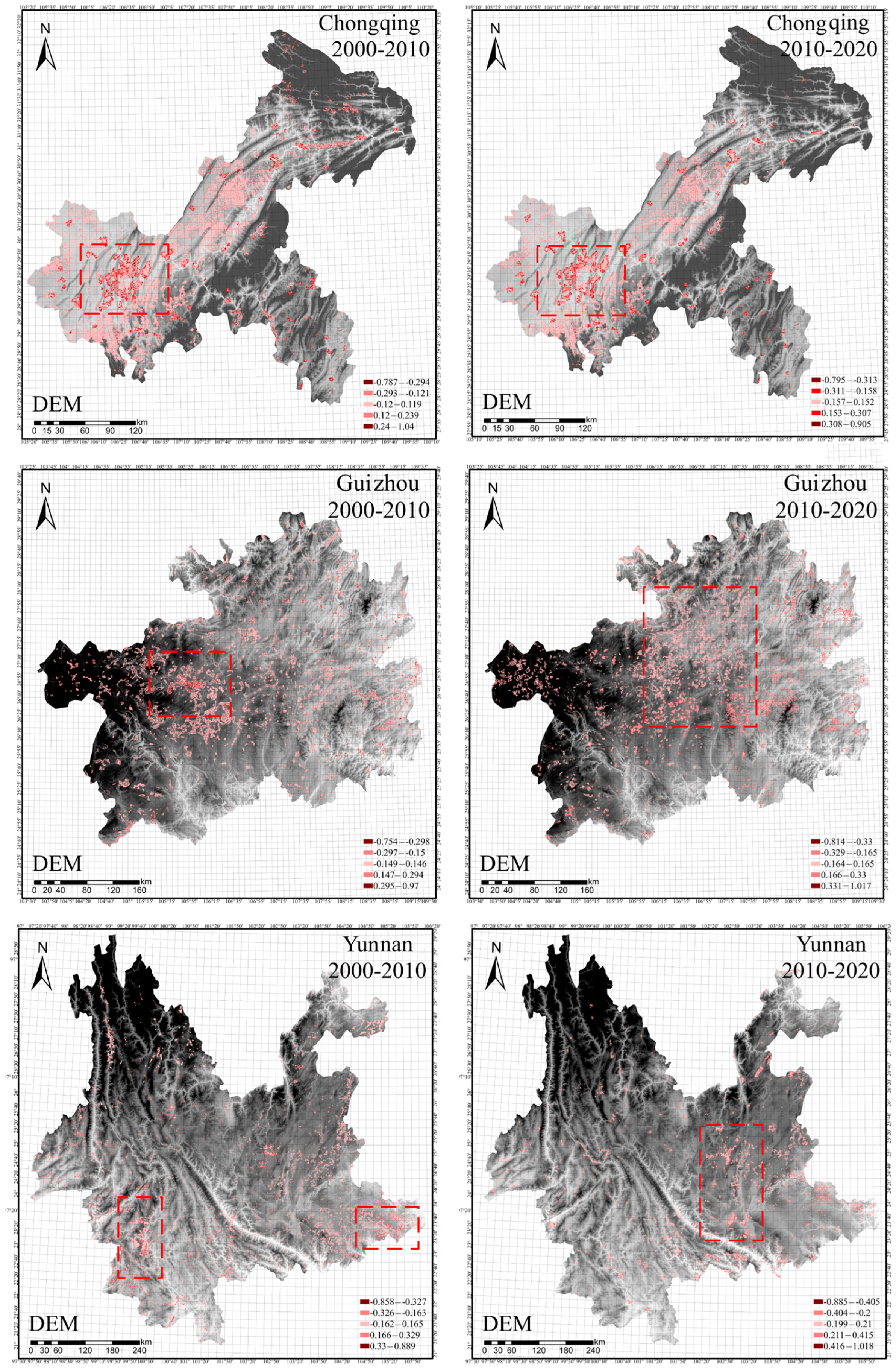
Because of the crucial importance of understanding the distribution pattern of residuals for evaluating the model’s applicability and verifying the assumptions, we specifically conducted a visual analysis of residuals in the GWR results with an R2 greater than 0.6 (As shown in Figure 7). Firstly, we categorized the residuals based on the range of a Gaussian distribution. Observing the legend, it is evident that the residuals in the GWR results have a mean of zero across different predicted values, indicating the absence of systematic bias throughout the entire dataset. Secondly, the residuals exhibit a spatial distribution of random and uniform patterns, aligning with the independence assumption of residuals.
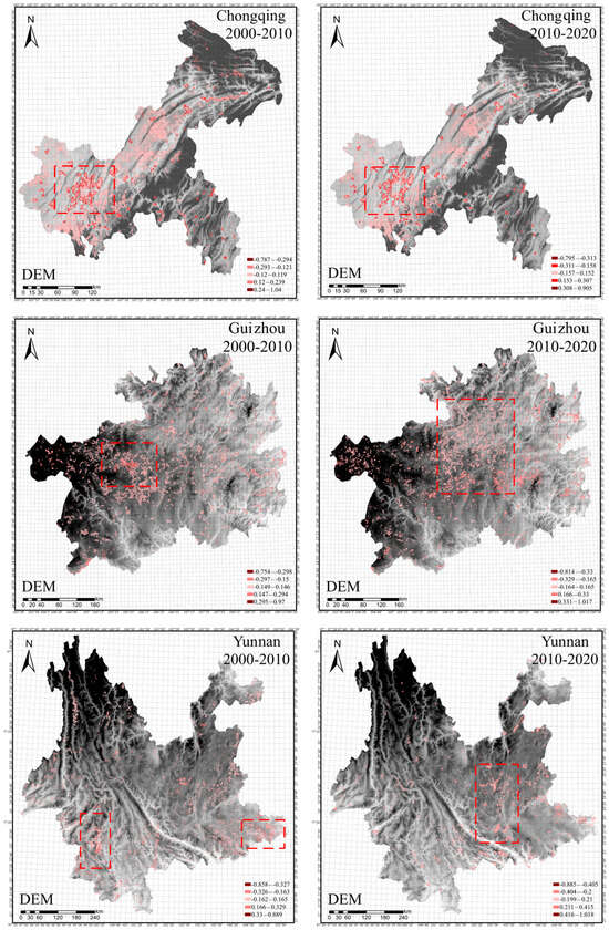
Figure 7.
Spatial distribution of residual during 2000–2010 and 2010–2020 in the three provinces considered in this study. The red boxes represent areas with high residuals across three regions over different time periods.
By comparing the spatial distribution of high residuals across the three provinces during the two time periods illustrated in Figure 7, we discerned variations in the distribution of model’s residual within localized regions of each province. This was accomplished by observing the red dotted line box in the figure and then deriving the change trend and degree of model performance in each province. In Chongqing, the spatial distribution of high residuals remained consistent, mainly concentrated in the main urban areas. The maximum and minimum values of the change amount were −0.135 and −0.008, respectively, suggesting the overall improvement of the model. In Guizhou, the dispersion of high residuals was more pronounced in the 2010–2020 period compared with the 2000–2010 period. The maximum and minimum values had a variation of 0.047 and −0.06, respectively, which suggests that the variability among localized regions may have been enhanced by changes in data quality or new influencing factors. However, there was no significant change in the overall performance of the model. In Yunnan, during 2000–2010, high residuals were concentrated in the southwest and southeast regions; however, in the 2010–2020 period, the distribution shifted to the central region. Meanwhile, the change in the maximum and minimum values of the residuals was 0.129 and −0.027, respectively. These changes indicate that the regional specificity of the central Yunnan region was stronger during this period and the overall performance of the model decreased. Overall, the distribution of residuals showed spatial clustering, and the overall performance of the model was stable.
Our further spatial autocorrelation analysis, based on the results of Moran’s index and z-score (As shown in Table 5), revealed the presence of spatial autocorrelation in residuals, contributing to the validation of the reliability of the GWR model. The table shows that Moran’s I values for all regions are below 0.3, and the absolute values of the z-scores exceed 1.96. This indicates that the residuals exhibit a nearly completely random spatial distribution pattern. Such a result suggests that the model fits the data well, with the chosen variables and model structure adequately explaining the spatial variability in the data. The random distribution of residuals implies that these differences are due to random error rather than model inadequacy. The analysis of Moran’s I and z-scores confirms that the model successfully fits the spatial data.
Table 5.
Residuals: Moran’s index and z-score in the spatial correlation report.
4.4. Coefficient Ranges and Weights of Variables under the Well-Fitted GWR Results
Next, we proceeded to calculate the range of the coefficients (representing the relative importance) of the eight independent variables that satisfied the condition of having an R2 adjustment greater than 0.6 in the context of the agglomeration region (as shown in Table 6 and Table 7). Then, we conducted an analysis to determine the impact of each variable on the rate of arable land loss during various periods.
Table 6.
Coefficient ranges of variables among agglomeration regions in 2000–2010.
Table 7.
Coefficient ranges of variables among agglomeration regions in 2010–2020.
In the period from 2000 to 2010, the Chongqing Northeast Yangtze River Basin and Zhong County exhibited the highest population coefficients, reaching −469.6 and −262.6, respectively, outdistancing the extremums of the other coefficients. In Chongqing Southwest Main City, the variable with the most significant coefficient range was the distance to urban areas, reaching 1536.3. In Guizhou, Guiyang showed substantial ranges for both the population and GDP coefficients, with values of 403.2 and 428.6, respectively. In contrast, Wanfeng Lake in Guizhou Province had relatively smaller ranges for the population and GDP coefficients, while the coefficient range for the distance to roads was the highest at 52.4, followed by GDP. In Yunnan, Lancang River Basin and Nanpan River Basin had population and GDP coefficients as their maximum values, significantly surpassing the other parameters with extremum values of 1878.6, 9381.6, and 1903.2, 39,085, respectively. The varying coefficient ranges for the other factors suggested significant changes in the overall influence of different factors in these regions. In the Wujiang River Basin, the rain and distance to urban coefficients had relatively larger ranges, exceeding 200.
In the period from 2010 to 2020, Chongqing Jiangjin District, Zhong County, and Southwest Main City exhibited the highest population and GDP coefficient ranges, surpassing 200,000. Similarly, Guizhou Guiyang and surrounding counties had the highest ranges for population and GDP coefficients, with the coefficient range for distance to urban areas at a comparable level. Additionally, Yunnan Kunming, Yuanjiang River Basin, Honghe Hani, and Yi Autonomous Prefecture all showed the highest ranges for population and GDP coefficients, while the coefficient ranges for other environmental factors varied, with the low coefficients range relatively. Analyzing coefficient ranges provided crucial insights into the changing factors influencing land loss in different regions over time, allowing for a deeper understanding of the impacts of factors such as population distribution and economic development on land loss.
This study standardized the mean, variance, and range of the variable coefficients and then calculated the annual mean values of these three metrics across different regions as weights to analyze changes in the factors influencing farmland degradation over a decade. As shown in Table 8, during the 2000–2010 period, environmental factors had influence weights concentrated between 0.3 and 0.6 in most regions, with rain being the primary influencing factor in the Wujiang area of Yunnan. However, after 2010, the influence of environmental factors generally declined to around 0.1, with a maximum of 0.2, and in the vicinity of Guiyang, Guizhou, the weight of environmental factors decreased significantly to below 0.02, indicating a minimal impact of environmental factors on farmland degradation. In contrast, population factors consistently influenced farmland degradation over the past 20 years. During the 2000–2010 period, the dominant population factors varied across the three regions as follows: in Chongqing, population and proximity to urban areas were the primary factors; in Guizhou, GDP and proximity to roads were predominant; while in Yunnan, GDP was the main influencing factor. Between 2010 and 2020, GDP and population became the dominant factors influencing farmland degradation in Chongqing and Yunnan. In Guiyang, proximity to urban areas and GDP had the greatest influence, while the influence weight of the population decreased to 0.043. More descriptive statistics on independent variable coefficients and R2 distributions can be found in Supplementary Materials.
Table 8.
Coefficient weights of variables among agglomeration regions generated via GWR-CUDA.
5. Discussion
5.1. The Factor Effect and Spatial Distribution of Good GWR-CUDA Fitting Results
5.1.1. Factor Effect of the High R2 Value Clusters
The first high R2 agglomeration regions were characterized by a predominant industry landscape. These regions rely heavily on manufacturing as their primary economic sector. In the early days of economic development, population and GDP were not the determining factors for land loss in these regions. Instead, factors such as urban and road construction played a decisive role in both the distribution and loss of arable land. A typical area is near the southwest main city, Chongqing, where the main factor affecting the loss of arable land was the distance from the city before 2010. The rationale may be that Chongqing is a significant player in heavy industry within China. This area mainly participates in transportation equipment, the chemical industry, heavy metal manufacturing, and other industries. As a result, the development of heavy industry inevitably led to the construction of factories, which made the distance to urban become the main factor affecting the loss of arable land.
Second, the high R2 spatial agglomeration areas were situated in highly urbanized densely populated urban agglomerations. In these regions, tertiary industries have replaced agriculture and industry as the key industries. As a result, GDP, population, and infrastructure were the predominant factors influencing land loss. The population and GDP, for 2010–2020, were the two main variables influencing the loss of arable land in all areas. For example, during this time, Kunming’s population grew from 6.439 million in 10 years to 8.463 million, and its GDP quadrupled, going from 216.59 billion to 673.38 billion. Rapid urbanization led to a population explosion and rapid urban growth. Similar regions included the main urban center of Chongqing.
Finally, the regions exhibited a notable concentration of R2 along rivers and lakes with relatively flat terrain. This was exemplified by the Zhong county in the Chongqing region, and Wanfeng Lake, which served as the origin of the Nanpan rivers in Guizhou Province before 2010. These regions provide abundant natural water supplies and flat topography that is conducive to agricultural activities. While topography, slope, and the distribution of rivers are outward factors influencing the loss of arable land [39], the allocation of water resources often influences the spatial distribution of populations and the developmental patterns of municipalities. Hence, specific agglomeration zones with high R2 values are influenced by varying degrees of environmental and human factors.
Based on the above analysis, the main factors in the high R2 agglomeration regions are also different. This illustrates that the non-smoothness of geographical factors in space causes different effects on the loss of arable land in different regions, reflecting characteristics such as spatial heterogeneity in the GWR model, which is helpful in explaining the different causes in different regions.
5.1.2. Reasons behind Different Periods of the Same High R2 Spatial Agglomeration Area
On the studied time scale, the same area will go through different development stages at different times because the economic level, the population, and the intervention of human activities will affect the factors of arable land loss. Thus, the leading causes of the same high R2 agglomeration area at different stages will be different. The main factor affecting the high R2 agglomeration area in Chongqing from 2000 to 2010 was the distance from the urban and some environmental factors, while the main factors affecting the high R2 agglomeration area from 2010 to 2020 were population, GDP, and the distance to urban.
The primary urban region in southwestern Chongqing experienced initial stages of urbanization between 2000 and 2010. During this period, cities were mainly developed by agriculture or industry, with a relatively stable population ranging from 28 to 29 million individuals. The city’s GDP exhibited gradual growth, increasing from RMB 0.2 trillion to RMB 0.81 trillion. To achieve significant economic growth, the development of infrastructure and the progressive urban expansion resulted in a significant loss of arable land near the city. This phenomenon may be attributed to the fact that the distance to urban areas and roads was identified as the primary contributing element. The current state of population growth and GDP indicates a period of stable and gradual development, resulting in a very limited influence on the loss of arable land.
In contrast, the main urban area in southwest Chongqing from 2010 to 2020 developed into the modern city stage, with a high level of economic development and urbanization, and the pillar industries mainly changed from agriculture and industry to tertiary industry. The GDP increased from 0.81 trillion to 2.5 trillion during this period, which was more than 2.5 times the previous decade. The rapid development of the economic level attracted many external populations, and the population of Chongqing increased from 28.846 million to 32.089 million. The high GDP and the population surge will increase the need for infrastructure such as housing, hospitals, shopping malls, etc., so arable land may be used for urban construction. It is worth noting that the distance to the city had an enhanced impact on the loss of arable land in the high R2 agglomeration area, indicating that the urban agglomeration in this high R2 agglomeration area is still expanding and has a high impact on the arable land around the city.
According to the study by He et al. [40], the impact of technological investment and government policies on land loss is significant. Before 2010, agricultural production in Chongqing primarily relied on manual labor, with low levels of technological application and minimal government intervention in land planning. Consequently, arable land loss was mainly influenced by environmental factors such as rain and evaporation. However, from 2010 to 2020, the Chongqing Municipal Government implemented the “Chongqing Land Consolidation Plan”, which focused on increasing investment in technology and capital to improve land quality, enhance the efficiency of land use, and strengthen agricultural infrastructure. This shift underscores the close relationship between land loss and human factors. The aforementioned research demonstrates that the influence on a specific agglomeration region with a high R2 varies across different temporal scales as a result of alterations in geographic factors. This research facilitates the anticipation of future alterations in causes contributing to the loss of arable land in comparable high R2 agglomeration regions. Consequently, it enables the formulation of robust interventions aimed at safeguarding against arable land loss and achieving a harmonious equilibrium between urban development and arable land conservation.
5.2. Limitations of the Model
During the process of selecting independent variables, we conducted a local collinearity diagnosis using the “gwr.collin.diagno” function for rain, temperature, and evaporation variables. This study revealed that VIF values for variables above 5 occurred in nearly half of the data points, indicating significant collinearity in certain local regions. To ensure the interpretability of variables with respect to the dependent variable, we retained rain and temperature while excluding the temperature variable with the smallest VIF variance. A lower variance in the temperature variable suggests more stable collinearity across different data points. Nonetheless, the presence of collinearity among variables, to a greater or lesser extent, remains a challenge affecting the current model’s performance.
Additionally, in the data processing section of this study, the transformation of the land loss issue from a binary variable to a continuous variable through the construction of a fishnet introduces the Modifiable Areal Unit Problem (MAUP). MAUP is a source of statistical bias that can significantly impact the results of statistical hypothesis tests. It affects results when point-based measures of spatial phenomena are aggregated into districts. The resulting summary values were influenced by both the shape and scale of the aggregation unit when we created the fishnet. Although in subsequent fishnet spatial analysis, we carefully selected grid parameters and appropriately determine grid size and orientation to minimize the impact of scale effects, the MAUP issue was still an unavoidable factor affecting the interpretability of the model.
6. Conclusions
This study addresses a critical knowledge gap related to the need for a comprehensive interpretation of the spatial distribution of results from the geographically weighted regression (GWR) model, an aspect that has been overlooked in prior research. By calculating Moran’s I index and visually representing local results, this research centers on analyzing the agglomeration phenomenon characterized by high R2 values. Specifically, it examines the context of arable land loss in the southwestern region of China over the past two decades, with a specific focus on Yunnan, Chongqing, and Guizhou Provinces. The primary objective is to explore the spatial distribution and underlying factors contributing to the variance in R2 values. This study can enhance the interpretability of the GWR model and provide insights into the spatial heterogeneity in the GWR model. The experimental results reveal a significant regional clustering of high R2 (>0.6) covering an area of approximately 102,166.76 (more than 40% of the total data on average), highlighting the importance of considering spatial heterogeneity in analyzing the factors contributing to land use change. Additionally, this research innovatively presents a novel approach for handling extensive datasets using the GWR model in the GIScience field. In addition to boosting the GWR model’s capacity to handle large-scale data, this research introduces an innovative approach to enhance the spatial interpretability of GWR by analyzing spatial clustering phenomena in its local results. This improvement allows for more targeted analyses of future GWR model applications, thereby broadening its applicability.
The findings of this research have noteworthy implications. According to the study results, high-R-squared agglomeration regions were concentrated within different regions according to the influence of different factors. Firstly, regions where industry remained the predominant industry exhibited a high correlation between arable land loss and the distance to urban. Secondly, areas characterized by higher population density and GDP in urban regions tended to experience lesser losses in arable land. This trend is attributed to the transition from agriculture and industry to tertiary industries, resulting in the limited availability of agricultural land in urban areas. Furthermore, this research underscores the influence of various factors, such as population, rain, evaporation, and slope, on arable land loss along river systems, highlighting the temporal variations in these influences. This study not only applies CUDA-enhanced GWR to analyze large-scale arable land loss efficiently but also offers a replicable solution for understanding spatial heterogeneity in regions worldwide. Traditional GWR models often face challenges when handling large datasets, especially in areas with complex interactions between environmental factors and human activities. By utilizing CUDA on high-performance GPU servers, this study enables efficient GWR computation, making it feasible to analyze extensive regions with diverse climatic, topographical, and socioeconomic conditions. Regions with high R2 clustering indicate strong explanatory power for arable land loss, allowing researchers to leverage this insight to predict future depletion. By examining the influence weights of various independent variables within these clustered regions and correlating them with the stages of economic development and environmental protection measures, researchers can quickly identify spatial distribution patterns of arable land loss and assess its spatial heterogeneity. Furthermore, the method’s visualization and spatial autocorrelation tools offer deeper insights into key drivers such as climate change, land use practices, and policy interventions. This provides a scientific foundation for developing more targeted land management and conservation strategies.
However, it is essential to acknowledge the limitations of this research. The reliance on raster data and the use of grid-based methodologies may overlook fine-scale variations and localized effects. Future research directions could involve the incorporation of more extensive land cover data and the exploration of alternative machine learning techniques to enhance the accuracy of predicting influential factors contributing to arable land loss.
Supplementary Materials
The following supporting information can be downloaded at https://www.mdpi.com/article/10.3390/agriculture14101675/s1, Table S1: the average value, variance, and range of independent variables coefficients; Table S2: the statistics for adjusting R2; Table S3: coefficients range visualization of independent variables.
Author Contributions
Conceptualization, T.X.; data curation, C.L., L.H. and A.T.; formal analysis, L.H. and A.T.; funding acquisition, T.X.; methodology, C.L.; project administration, T.X.; resources, C.L. and S.D.; software, T.X.; validation, T.X.; visualization, S.D.; writing—original draft, C.L. and L.H.; writing—review and editing, T.X. All authors have read and agreed to the published version of the manuscript.
Funding
This work was supported by the Ministry of Natural Resources Key Laboratory of Digital Mapping and Land Information Application Open Research Fund [Project No: ZRZYBWD202303] and the “Overseas students’ innovation and entrepreneurship plan”, Chongqing, grant number CX2021065.
Institutional Review Board Statement
Not applicable.
Data Availability Statement
The data and codes that support the findings of this study are available with the identifier(s) at the private link https://figshare.com/s/7416e1d9bd47975c0259.
Conflicts of Interest
The authors declare that they have no known competing financial interests or personal relationships that could have appeared to influence the work reported in this paper.
References
- Ye, S.; Ren, S.; Song, C.; Cheng, C.; Shen, S.; Yang, J.; Zhu, D. Spatial patterns of county-level arable land productive-capacity and its coordination with land-use intensity in mainland China. Agric. Ecosyst. Environ. 2022, 326, 107757. [Google Scholar] [CrossRef]
- Liu, X.; Wang, S.; Zhuang, Q.; Jin, X.; Bian, Z.; Zhou, M.; Meng, Z.; Han, C.; Guo, X.; Jin, W.; et al. A Review on Carbon Source and Sink in Arable Land Ecosystems. Land 2022, 11, 580. [Google Scholar] [CrossRef]
- Prăvălie, R.; Patriche, C.; Borrelli, P.; Panagos, P.; Roșca, B.; Dumitraşcu, M.; Nita, I.-A.; Săvulescu, I.; Birsan, M.-V.; Bandoc, G. Arable lands under the pressure of multiple land degradation processes. A global perspective. Environ. Res. 2021, 194, 110697. [Google Scholar] [CrossRef] [PubMed]
- Fu, Z.; Cai, Y.; Yang, Y.; Dai, E. Research on the relationship of cultivated land change and food security in China. J. Nat. Resour. 2001, 16, 313–319. [Google Scholar]
- Larson, C. Losing Arable Land, China Faces Stark Choice: Adapt or Go Hungry. Science 2013, 339, 644–645. [Google Scholar] [CrossRef] [PubMed]
- Long, H.; Li, Y.; Liu, Y.; Woods, M.; Zou, J. Accelerated restructuring in rural China fueled by ‘increasing vs. decreasing balance’ land-use policy for dealing with hollowed villages. Land Use Policy 2012, 29, 11–22. [Google Scholar] [CrossRef]
- Qu, Q.-Y.; Yang, H.; Zhao, Y.-H.; Han, L. Temporal and spatial changes and its characteristics of cultivated land and grain yield in China from 2009 to 2017. Hubei Agric. Sci. 2022, 61, 29–34. [Google Scholar]
- Liu, J.; Guo, Q. A spatial panel statistical analysis on cultivated land conversion and chinese economic growth. Ecol. Indic. 2015, 51, 20–24. [Google Scholar] [CrossRef]
- Tu, Y.; Chen, B.; Yu, L.; Xin, Q.; Gong, P.; Xu, B. How does urban expansion interact with cropland loss? A comparison of 14 Chinese cities from 1980 to 2015. Landsc. Ecol. 2021, 36, 243–263. [Google Scholar] [CrossRef]
- Tu, Y.; Chen, B.; Yu, L.; Song, Y.; Wu, S.; Li, M.; Wei, H.; Chen, T.; Lang, W.; Gong, P.; et al. Raveling the nexus between urban expansion and cropland loss in China. Landsc. Ecol. 2023, 38, 1869–1884. [Google Scholar] [CrossRef]
- Alexander, P.; Rounsevell, M.D.A.; Dislich, C.; Dodson, J.R.; Engström, K.; Moran, D. Drivers for global agricultural land use change: The nexus of diet, population, yield and bioenergy. Glob. Environ. Chang. 2015, 35, 138–147. [Google Scholar] [CrossRef]
- Song, W.; Pijanowski, B.C.; Tayyebi, A. Urban expansion and its consumption of high-quality farmland in Beijing, China. Ecol. Indic. 2015, 54, 60–70. [Google Scholar] [CrossRef]
- Saturday, A. Restoration of Degraded Agricultural Land: A Review. J. Environ. Health Sci. 2018, 4, 44–51. [Google Scholar]
- Mansour, S.; Al Kindi, A.; Al-Said, A.; Al-Said, A.; Atkinson, P. Sociodemographic determinants of COVID-19 incidence rates in Oman: Geospatial modelling using multiscale geographically weighted regression (MGWR). Sustain. Cities Soc. 2021, 65, 102627. [Google Scholar] [CrossRef]
- Tasyurek, M.; Celik, M. 4D-GWR: Geographically, altitudinal, and temporally weighted regression. Neural Comput. Appl. 2022, 34, 14777–14791. [Google Scholar] [CrossRef]
- Khalid, S.; Zameer, F. Revisiting Urban Immovable Property Valuation: An Appraisal of Spatial Heterogeneities in Punjab Using Big Data. Pak. Dev. Rev. 2023, 62, 493–520. [Google Scholar] [CrossRef]
- Lu, C.; Ma, L.; Liu, T.-X.; Huang, X. Temporal and spatial variations of annual precipitation and meteorological drought in China during 1951–2018. Chin. J. Appl. Ecol. 2022, 33, 1572–1580. [Google Scholar]
- Liu, C.; Wu, X.; Wang, L. Analysis on land ecological security change and affect factors using RS and GWR in the Danjiangkou Reservoir area, China. Appl. Geogr. 2019, 105, 1–14. [Google Scholar] [CrossRef]
- Yu, H.; Gong, H.; Chen, B.; Liu, K.; Gao, M. Analysis of the influence of groundwater on land subsidence in Beijing based on the geographical weighted regression (GWR) model. Sci. Total Environ. 2020, 738, 139405. [Google Scholar] [CrossRef] [PubMed]
- Lu, B.; Hu, Y.; Murakami, D.; Brunsdon, C.; Comber, A.; Charlton, M.; Harris, P. High-performance solutions of geographically weighted regression in R. Geo-Spat. Inf. Sci. 2022, 25, 536–549. [Google Scholar] [CrossRef]
- Tian, A.; Xu, T.; Gao, J.; Liu, C.; Han, L. Multi-scale spatiotemporal wetland loss and its critical influencing factors in China determined using innovative grid-based GWR. Ecol. Indic. 2023, 149, 110144. [Google Scholar] [CrossRef]
- Wang, C.; Li, S.; Shan, J. Non-Stationary Modeling of Microlevel Road-Curve Crash Frequency with Geographically Weighted Regression. ISPRS Int. J. Geo-Inf. 2021, 10, 286. [Google Scholar] [CrossRef]
- Wang, D.; Yang, Y.; Qiu, A.; Kang, X.; Han, J.; Chai, Z. A CUDA-Based Parallel Geographically Weighted Regression for Large-Scale Geographic Data. ISPRS Int. J. Geo-Inf. 2020, 9, 653. [Google Scholar] [CrossRef]
- Tian, M.; Wang, X.; Wang, Q.; Qiao, Y.; Wu, H.; Hu, Q. Geographically weighted regression (GWR) and Prediction-area (P-A) plot to generate enhanced geochemical signatures for mineral exploration targeting. Appl. Geochem. 2023, 150, 105590. [Google Scholar] [CrossRef]
- Li, M.; Zhang, C.; Xu, B.; Xue, Y.; Ren, Y. A comparison of GAM and GWR in modelling spatial distribution of Japanese mantis shrimp (Oratosquilla oratoria) in coastal waters. Estuar. Coast. Shelf Sci. 2020, 244, 106928. [Google Scholar] [CrossRef]
- Getayeneh Antehunegn, T.; Lemma Derseh, G.; Solomon Gedlu, N. Spatial distribution of stillbirth and associated factors in Ethiopia: A spatial and multilevel analysis. BMJ Open 2020, 10, e034562. [Google Scholar]
- Tu, J.; Xia, Z.-G. Examining spatially varying relationships between land use and water quality using geographically weighted regression I: Model design and evaluation. Sci. Total Environ. 2008, 407, 358–378. [Google Scholar] [CrossRef]
- Wang, L.; Anna, H.; Zhang, L.; Xiao, Y.; Wang, Y.; Xiao, Y.; Liu, J.; Ouyang, Z. Spatial and Temporal Changes of Arable Land Driven by Urbanization and Ecological Restoration in China. Chin. Geogr. Sci. 2019, 29, 809–819. [Google Scholar] [CrossRef]
- Liu, N.; Strobl, J. Impact of neighborhood features on housing resale prices in Zhuhai (China) based on an (M)GWR model. Big Earth Data 2023, 7, 146–169. [Google Scholar] [CrossRef]
- Nazeer, M.; Bilal, M. Evaluation of Ordinary Least Square (OLS) and Geographically Weighted Regression (GWR) for Water Quality Monitoring: A Case Study for the Estimation of Salinity. J. Ocean Univ. China 2018, 17, 305–310. [Google Scholar] [CrossRef]
- Mahara, D.; Fauzan, A. Impacts of Human Development Index and Percentage of Total Population on Poverty using OLS and GWR models in Central Java, Indonesia. EKSAKTA J. Sci. Data Anal. 2021, 2, 142–154. [Google Scholar] [CrossRef]
- Dong, W.; Ge, W.-C.; Chen, K.-L. Application Research of CUDA Parallel Computing. Inf. Technol. 2010, 34, 11–15. [Google Scholar]
- Liu, Y.; Xie, Y.; Yang, W.; Zuo, X.; Ge, Q.; Zhou, B. Target Classification and Recognition for High-Resolution Remote Sensing Images: Using the Parallel Cross-Model Neural Cognitive Computing Algorithm. IEEE Geosci. Remote Sens. Mag. 2020, 8, 50–62. [Google Scholar] [CrossRef]
- Owens, J.D.; Houston, M.; Luebke, D.; Green, S.; Stone, J.E.; Phillips, J.C. GPU Computing. Proc. IEEE 2008, 96, 879–899. [Google Scholar] [CrossRef]
- Li, Z.; He, W.; Cheng, M.; Hu, J.; Yang, G.; Zhang, H. SinoLC-1: The first 1 m resolution national-scale land-cover map of China created with a deep learning framework and open-access data. Earth Syst. Sci. Data 2023, 15, 4749–4780. [Google Scholar] [CrossRef]
- Kumari, M.; Sarma, K.; Sharma, R. Using Moran’s I and GIS to study the spatial pattern of land surface temperature in relation to land use/cover around a thermal power plant in Singrauli district, Madhya Pradesh, India. Remote Sens. Appl. Soc. Environ. 2019, 15, 100239. [Google Scholar] [CrossRef]
- Nakagawa, S.; Schielzeth, H. A general and simple method for obtaining R2 from generalized linear mixed-effects models. Methods Ecol. Evol. 2013, 4, 133–142. [Google Scholar] [CrossRef]
- Getis, A. Reflections on spatial autocorrelation. Reg. Sci. Urban Econ. 2007, 37, 491–496. [Google Scholar] [CrossRef]
- Tang, J.-L.; Cheng, X.-Q.; Zhu, B.; Gao, M.; Wang, T.; Zhang, X.-F.; Zhao, P.; You, X. Rainfall and tillage impacts on soil erosion of sloping cropland with subtropical monsoon climate—A case study in hilly purple soil area, China. J. Mt. Sci. 2015, 12, 134–144. [Google Scholar] [CrossRef]
- He, P.; Wang, Q.-C.; Shen, G.Q. The Carbon Emission Implications of Intensive Urban Land Use in Emerging Regions: Insights from Chinese Cities. Urban Sci. 2024, 8, 75. [Google Scholar] [CrossRef]

Disclaimer/Publisher’s Note: The statements, opinions and data contained in all publications are solely those of the individual author(s) and contributor(s) and not of MDPI and/or the editor(s). MDPI and/or the editor(s) disclaim responsibility for any injury to people or property resulting from any ideas, methods, instructions or products referred to in the content. |
© 2024 by the authors. Licensee MDPI, Basel, Switzerland. This article is an open access article distributed under the terms and conditions of the Creative Commons Attribution (CC BY) license (https://creativecommons.org/licenses/by/4.0/).