Chinese Bayberry Detection in an Orchard Environment Based on an Improved YOLOv7-Tiny Model

Abstract

The precise detection of Chinese bayberry locations using object detection technology is a crucial step to achieve unmanned harvesting of these berries. Because of the small size and easy occlusion of bayberry fruit, the existing detection algorithms have low recognition accuracy for such objects. In order to realize the fast and accurate recognition of bayberry in fruit trees, and then guide the robotic arm to carry out accurate fruit harvesting, this paper proposes a detection algorithm based on an improved YOLOv7-tiny model. The model introduces partial convolution (PConv), a SimAM attention mechanism and SIoU into YOLOv7-tiny, which enables the model to improve the feature extraction capability of the target without adding extra parameters. Experimental results on a self-built Chinese bayberry dataset demonstrate that the improved algorithm achieved a recall rate of 97.6% and a model size of only 9.0 MB. Meanwhile, the precision of the improved model is 88.1%, which is 26%, 2.7%, 4.7%, 6.5%, and 4.7% higher than that of Faster R-CNN, YOLOv3-tiny, YOLOv5-m, YOLOv6-n, and YOLOv7-tiny, respectively. In addition, the proposed model was tested under natural conditions with the five models mentioned above, and the results showed that the proposed model can more effectively reduce the rates of misdetections and omissions in bayberry recognition. Finally, the improved algorithm was deployed on a mobile harvesting robot for field harvesting experiments, and the practicability of the algorithm was further verified.

1. Introduction

The Chinese bayberry is a common subtropical fruit with a spherical shape, widely cultivated in the southern regions of China [1]. It is highly favored by the Chinese people for its delicious and juicy taste, as well as its medicinal value [2]. However, Chinese bayberry trees are tall and mainly grown in hilly areas, so manual harvesting poses risks of falling. Additionally, Chinese bayberry fruits have a short ripening period and are sensitive to environmental influences, making the time available for manual harvesting short [3]. These challenges have somewhat constrained the development of the Chinese bayberry industry. In recent years, various devices have been utilized for fruit harvesting [4,5]; however, these devices mainly vibrate the fruit trees for the harvesting of fruit and lack sufficient automation. Therefore, research on automatic bayberry harvesting robots holds great practical significance.

The image detection system is a crucial component of an automatic bayberry harvesting robot, which can only control the actuator to realize automatic picking by accurately recognizing the position of the bayberry [6,7]. Currently, detection algorithms are mainly classified as either traditional [8,9] or deep learning-based [10,11]. Traditional image detection algorithms first select candidate regions in the image, then extract features from these regions, and finally classify them using a trained classifier. These algorithms suffer from window redundancy, long processing times, and poor robustness in complex orchard environments, making them insufficient to meet harvesting requirements.

In recent years, with advancements in computer science and the refinement of deep learning theories, deep learning-based object detection algorithms [12,13,14] have gradually replaced traditional image detection algorithms. Deep learning object detection algorithms can be categorized into two types: two-stage and one-stage. Two-stage object detection algorithms first generate candidate regions in the image and then locate and regress the boundaries of the target in these regions. Common two-stage detection algorithms include Fast regions with a convolutional neural network (Fast R-CNN) [15], Faster regions with a convolutional neural network (Faster R-CNN) [16], and Mask regions with a convolutional neural network (Mask R-CNN) [17]. Yu et al. (2019) [18] utilized Resnet50 as the backbone network, exploring a strawberry detection algorithm based on Mask R-CNN. Experimental results demonstrated that the model achieved an average precision of 95.78%. Liu et al. (2019) [19] applied Faster R-CNN to persimmon detection, proposing an improved Faster R-CNN detection algorithm. This method used Deterministic Networking (DetNet) as the backbone network and added the Efficient Channel Attention (ECA) attention mechanism to effectively perform persimmon detection in complex environments. Although two-stage object detection algorithms generally have high precision, they are slow. One-stage object detection algorithms do not require the selection of candidate regions; they directly divide the image into multiple small regions and perform feature extraction, target classification, and localization in each small region. You Only Look Once (YOLO) [20] and Single-Shot multiBox Detector (SSD) currently the mainstream one-stage detection algorithms.

Currently, owing to the high detection precision and short recognition time of the YOLO detection algorithms, many researchers have applied them to the field of agricultural harvesting robots. Ji et al. (2021) [21] used an improved YOLOv4 for apple detection in complex orchard environments. This model employed the EfficientNet network as the feature extraction network for apple recognition, reducing the model’s size. Cao et al. (2022) [22] proposed a YOLOv4-LightC-CBAM model for real-time mango detection. By adjusting the model’s network width and adding attention mechanisms, they improved the network’s detection precision. However, this algorithm was tested under dark conditions at night with a single background, and was hardly affected by environmental factors around the orchard. Sun et al. (2022) [23] introduced ShuffleNet and GhostNet structures into the YOLOv5 model and added an attention module, proposing a YOLOv5-PRE model for detecting apples in orchards. Experimental results demonstrated that the improved YOLOv5 model achieved an average precision of 94.03%. Li et al. (2023) [24] developed a recognition algorithm for tomatoes based on the improved YOLOv5s model. However, this algorithm was applied in indoor greenhouse environments and did not reflect real orchard conditions. Zhou et al. (2023) [25] introduced RepGhost and a decoupled head approach, proposing the RDE-YOLOv7 model for dragon fruit recognition. Experimental results showed that the RDE-YOLOv7 precision, recall rate, and average precision improved by 0.4%, 2.5%, and 0.8%, respectively, compared to those of YOLOv7. Chen et al. (2022) [26] introduced small target detection layers, GhostConv, and CBAM for citrus recognition based on the YOLOv7 model. Experimental results demonstrated that the improved YOLOv7 model achieved an average precision of 97.29% and an average detection time of 69.38 ms.

The above studies have contributed to the development of agricultural fruit detection. Fruit harvesting is part of precision agriculture, where image recognition is carried out in real time by the equipped camera sensor, which in turn controls the robotic arm for precise positioning and harvesting. Efficient recognition algorithms can improve the efficiency of mechanized agricultural harvesting and reduce manual intervention. However, Chinese bayberry fruits are small and densely packed, and the YOLO detection algorithm exhibits poor performance in detecting such small targets [27]. Recognition precision is easily affected by factors such as overlapping fruits, lighting conditions, and branches. Therefore, this paper proposes an improved YOLOv7-tiny algorithm for bayberry detection to address the existing recognition issues. In this study, partial convolution, SimAM and SIoU are introduced into the YOLOv7-tiny model to enhance the feature extraction capability of the model; the improved model was then deployed to a harvesting robot to perform mechanical harvesting in the field.

2. Materials and Methods

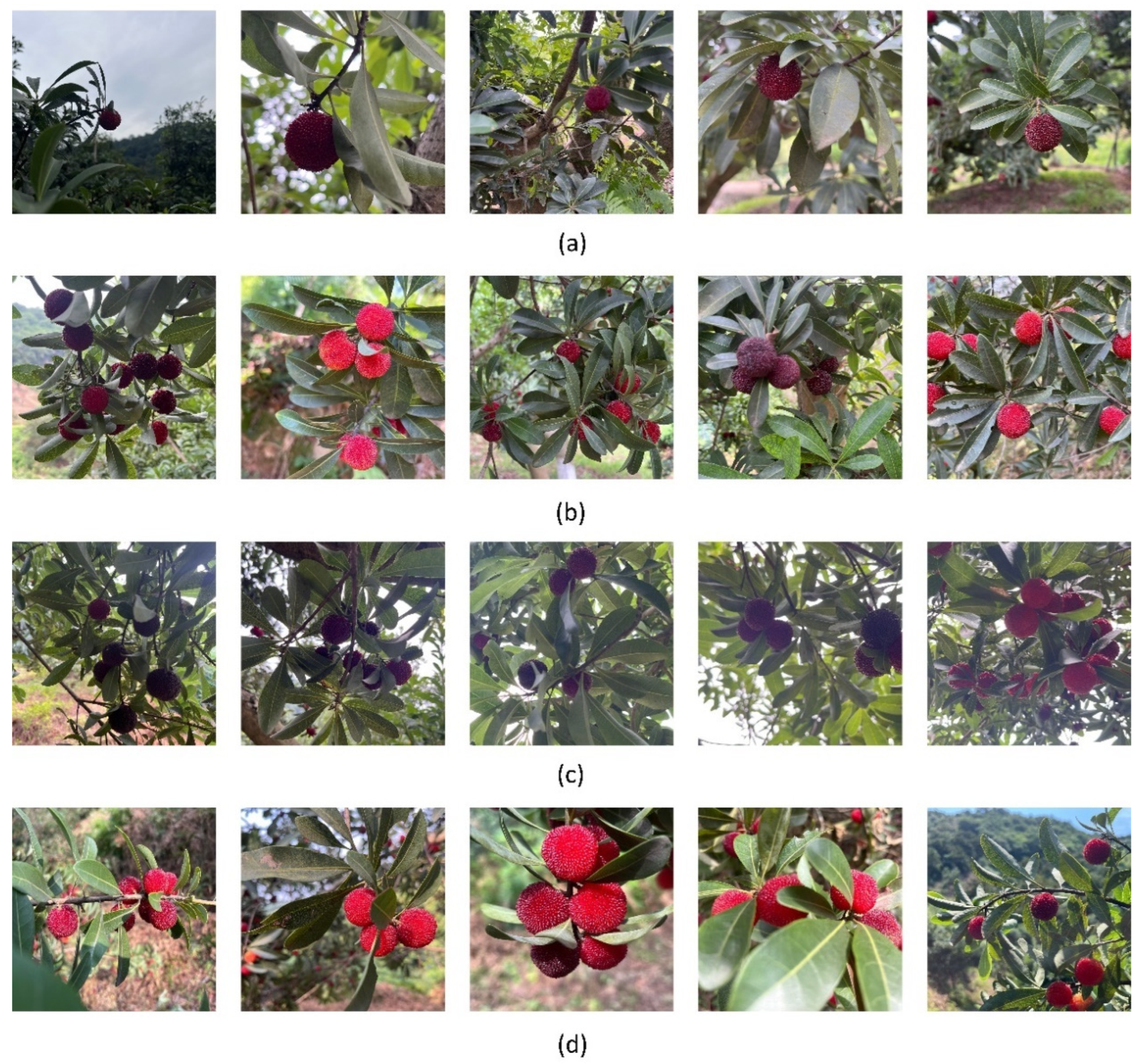
2.1. Bayberry Image Collection

The study used a self-built dataset of Chinese bayberry fruits in hilly environments. The images were captured in a renowned Chinese bayberry orchard in the Lanjiang Street, Yuyao, Ningbo city, Zhejiang province in eastern China. The bayberry trees in the orchard have an approximate spacing of 2–3 m and a height of approximately 3 m, meeting the requirements for intelligent robot harvesting. The data collection utilized an iPhone 13 for image capture, with an image resolution of 3024 × 4032 pixels. To ensure optimal dataset quality, the images were captured on 15 June and 16 June 2023, and 1200 images were obtained in total. To ensure the authenticity and diversity of the dataset, the captured images included cases with a single fruit, multiple fruits, backlight and light-facing environments, and sunny and cloudy scenes. Some samples of the dataset are illustrated in Figure 1.

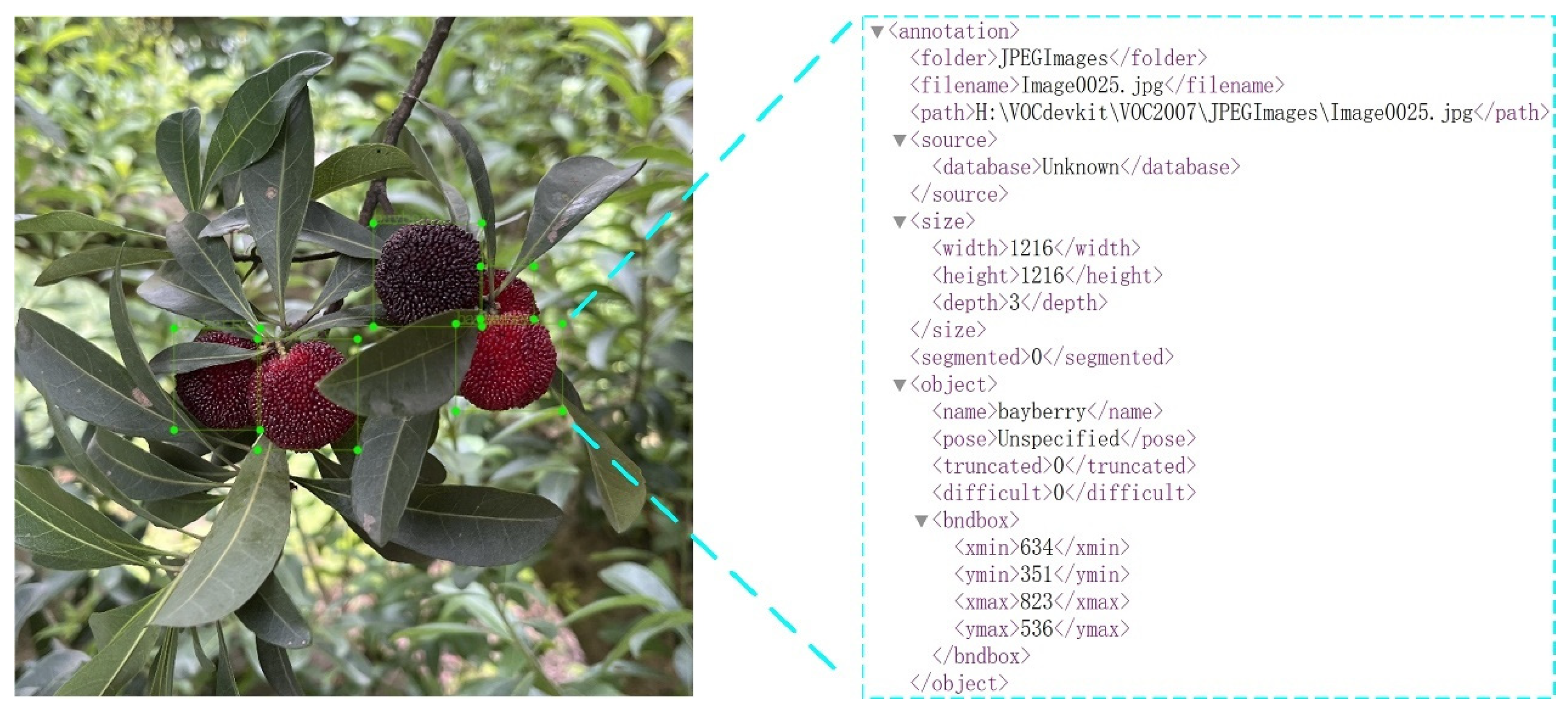
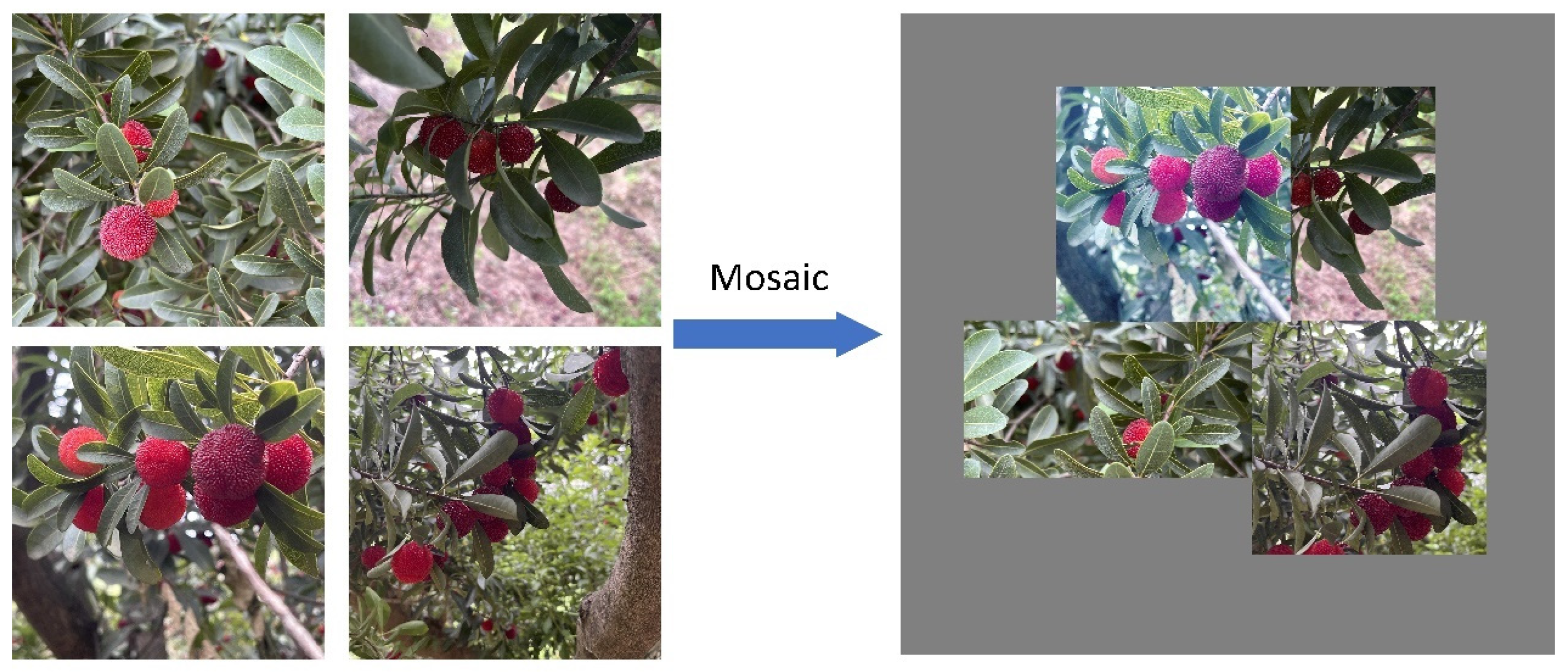
2.2. Data Annotation and Augmentation

To facilitate the training of the neural network model, it is imperative to annotate the acquired dataset. In this experiment, bayberries were annotated as a distinct class, and LabelImg 1.8.5 version annotation software was employed for manual annotation. An XML file was generated for each annotated image, encompassing the classifications of all labels, positions of the labels, and size of the image, as depicted in Figure 2.

A visual analysis of the annotated dataset files is presented in Figure 3. Figure 3a illustrates the distribution of the locations of labels in the dataset. The horizontal coordinate (x) represents the ratio of the horizontal coordinate of the label center to the image width, whereas the vertical coordinate (y) represents the ratio of the horizontal coordinate of the label center to the image height. As shown, there are a large number of bayberries in the self-built dataset and they are mainly distributed in the middle part of the image. Figure 3b illustrates the size distribution of labels in the dataset. The horizontal coordinate (width) represents the ratio of the label width to the image width, whereas the vertical coordinate (height) represents the ratio of the label height to the image height. As shown, the label height and width in the self-built dataset are less than 0.2 times the corresponding image dimensions in most cases; thus, the labeled items belong to the category of small targets, which aligns with real orchard conditions. Ultimately, the dataset of 1200 images was partitioned into training and testing sets in an 8:2 ratio.

By augmenting the dataset, we can not only effectively simulate the complex environments in real orchards, but also enhance the model’s generalization ability, preventing overfitting. This study applied the inherent mosaic data augmentation method of the YOLO model to enhance the training data, including combining four images into one (Mosaic), flipping the image horizontally (Fliplr), overlaying two images (Mixup), and enhancement of the image’s HSV in terms of hue, saturation, and value. Figure 4 illustrates the data augmentation process. The data augmentation enhances the diversity of the dataset, thus improving the model’s robustness. The hyperparameters for the data augmentation method are presented in

Table 1. The hyperparameter settings of data augmentation.

Hyperparameter	Value
Mosaic	100% probability
Fliplr	50% probability
Mixup	15% probability
HSV_Hue	0.015 fraction
HSV_Saturation	0.7 fraction
HSV_Value	0.4 fraction

.

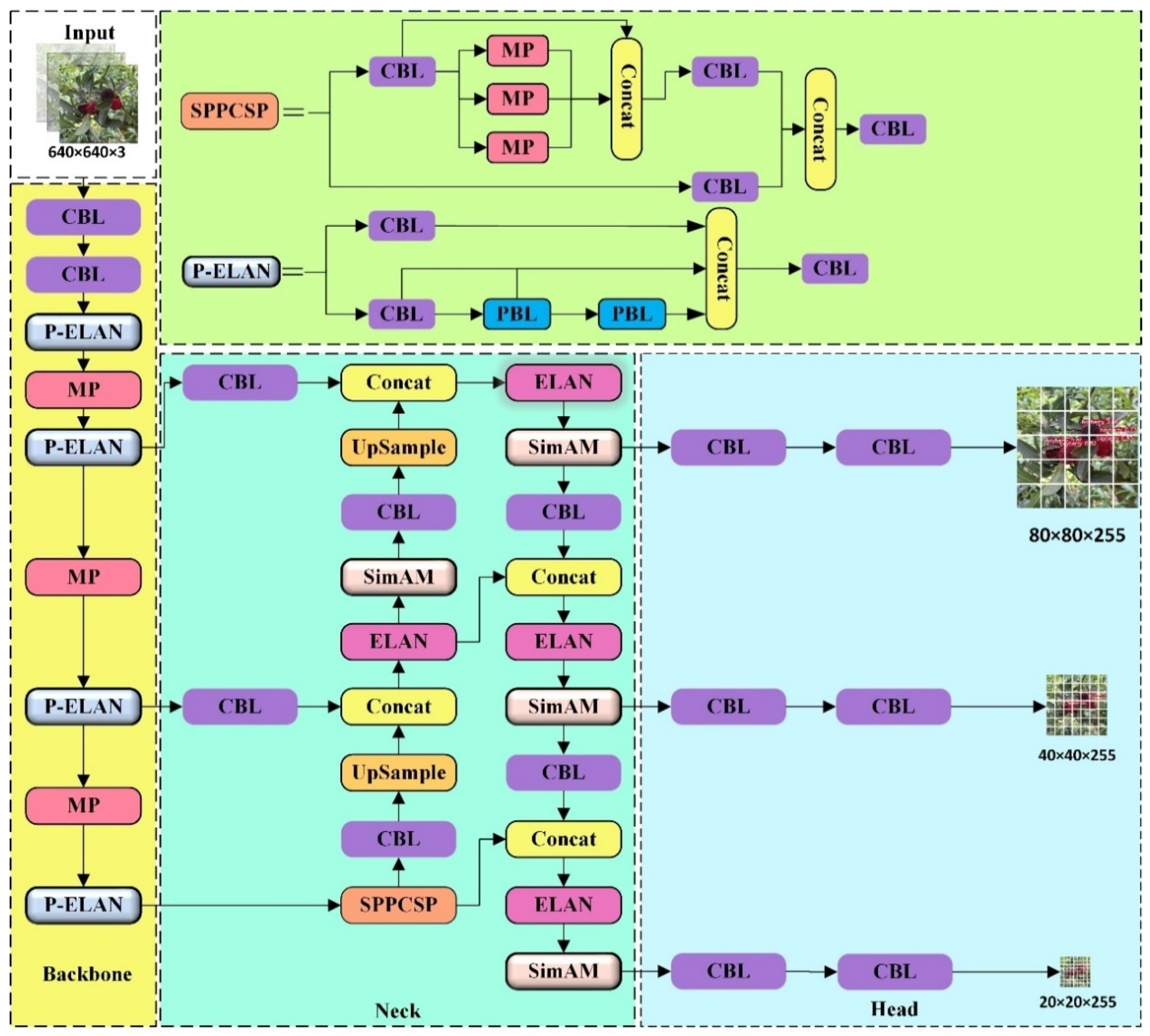
2.3. YOLOv7-Tiny Object Detection Network

YOLO algorithms are among the most popular object detection algorithms. Their simple network structure and high detection speed make them widely applicable for agricultural harvesting robots. YOLOv7, introduced by Wang et al. [28], is the latest detection algorithm in the YOLO series.

YOLOv7 employs a cascade-based model scaling approach to generate multiple architectures, including YOLOv7, YOLOv7-tiny, YOLOv7x, YOLOv7-w6, YOLOv7-e6, YOLOv7-e6e, and YOLOv7-d6. Regular GPU deployment is used for the former three networks, whereas the latter four networks are intended for high-performance cloud GPU deployment. In this study, a regular GPU was used, and the first three networks were individually trained. We use average precision (mAP), recall and model size as the evaluation metrics of the model. Average precision represents a combined assessment of precision and recall under category and detection thresholds and recall indicates the number of correctly detected targets as a percentage of the total number of targets. The results are presented in

Table 2. Comparison of the performance of different YOLOv7 models.

Model	mAP (%)	Recall (%)	Model Size (MB)
YOLOv7	91.9	94.5	73.1
YOLOv7-tiny	93.7	96.3	11.9
YOLOv7x	92.5	94.6	138.7

. As shown, YOLOv7-tiny outperformed the other two networks in terms of mean average precision, recall rate, and model size. Therefore, YOLOv7-tiny was selected for the subsequent experiment.

YOLOv7-tiny consists of four components: Input, Backbone, Neck, and Head. The Input side preprocesses each input image through procedures such as data augmentation and adaptive anchor box calculation, standardizing the image size to 640 × 640 × 3. The processed images are then fed into the Backbone layer. The Backbone layer serves as the feature extraction layer, comprising multiple CBL convolution modules, Efficient Layer Aggregation Network (ELAN) modules, and MP modules. The CBL convolution module, consisting of a Conv layer, a BN layer, and the Leaky ReLU activation function, extracts feature information from the images. The ELAN module is formed by combining multiple CBL modules through multiple branches to enhance the network’s learning ability. The MP module utilizes max-pooling operations for downsampling. The Neck layer acts as the feature fusion layer, incorporating SPPCSP modules, CBL modules, and ELAN modules. The SPPCSP module consists of two parts, SPP and CSP. SPP utilizes the maximum pooling of four different scales to achieve the fusion of information from different feature scales; CSP performs a concat operation to enrich feature information. This layer adopts a path aggregation feature pyramid network (PAFPN) structure, facilitating multi-scale fusion of the network through top-down and bottom-up approaches, which is advantageous for small object detection. The Head layer serves as the output prediction layer, where the three different-scale feature maps of the Neck layer output undergo adjustment of the image channel numbers, using convolution modules to predict the confidence, category, and anchor boxes.

2.4. Improvement of the YOLOv7-Tiny Network Model

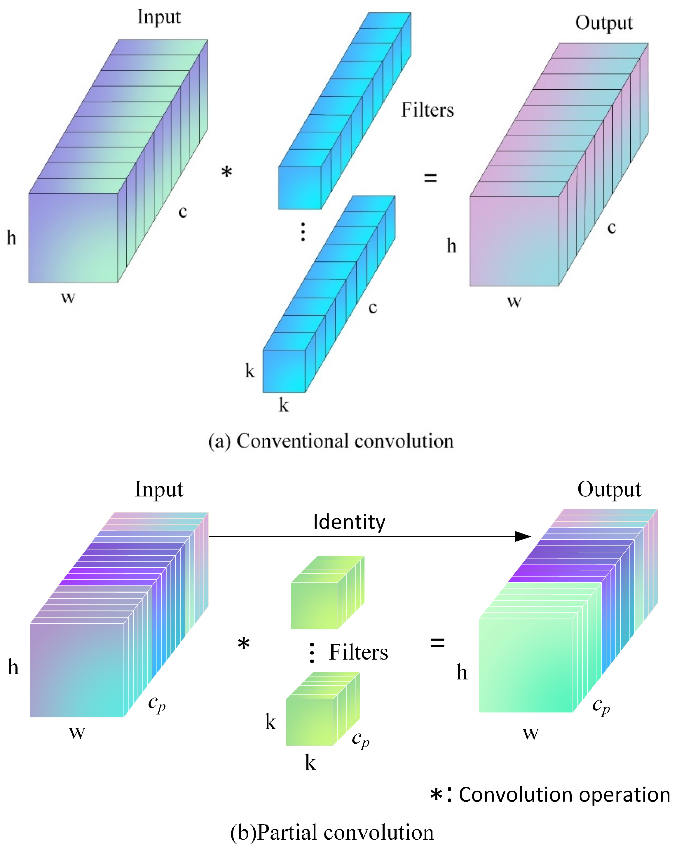
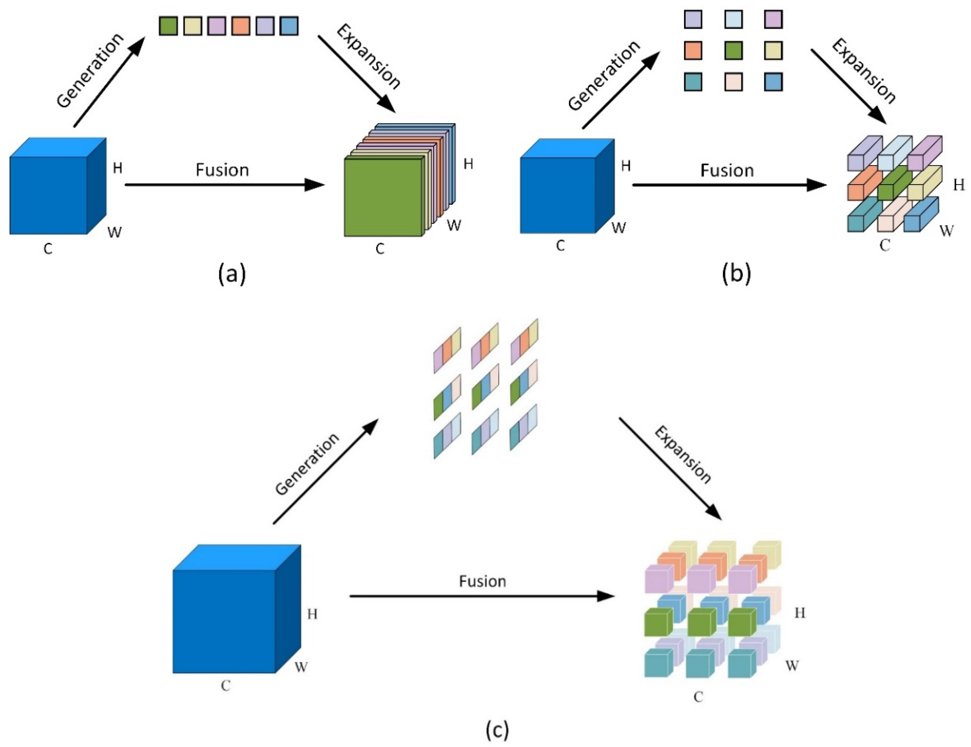
2.4.1. Improvement of the Backbone Network

The structural diagram of a conventional convolution is illustrated in Figure 5a. This convolution necessitates feature extraction for each input channel, increasing the model’s computational complexity and slowing down network operation. To enhance the speed of neural networks, previous studies have often used the number of floating-point operations (FLOPs) as an evaluation metric for the computational complexity of a model, and achieve the effect of reducing the computational complexity of the model by decreasing the FLOPs, such as Depthwise Convolution (DWConv) [29] and Ghost Convolution (Ghost Conv) [30]. However, a decrease in the number of FLOPs does not necessarily translate to an improvement in network operation speed. This is because the detection speed of the network is related not only to FLOPs but also to floating-point operations per second (FLOPS). To simultaneously reduce computational redundancy and memory access, enabling neural networks to maintain high FLOPS while reducing the number of FLOPs, Chen et al. [31] proposed a novel convolution module, partial convolution (PConv). PConv performs feature extraction with Conv only on a subset of input channels, without affecting the remaining channels, effectively avoiding computational redundancy in feature maps. For continuous or regular memory access, the first or last continuous channel is treated as the representative for the entire feature map to be calculated. The working mechanism of PConv is illustrated in Figure 5b.

In comparison to Conv, PConv only performs feature extraction on a certain number (c_p) of input channels, while retaining the original feature information in other channels. The number of FLOPs for Conv and PConv is calculated as in Equations (1) and (2).

$${\mathrm{FLOPs}}_{(\mathrm{Conv})}=k^2\times c^2\times h\times w=k^2{c}^{2}hw$$

(1)

$${\mathrm{FLOPs}}_{(\mathrm{PConv})}=k^2\times c_p^2\times h\times w=k^2{c}_p^{2}hw$$

(2)

where h is the height of the input feature, w is the width of the input feature, k is the size of the convolution kernel, c_p is the number of PConv channels, and c is the number of Conv channels. The memory access cost (MAC) for Conv and PConv is calculated as in Equations (3) and (4).

$${\mathrm{MAC}}_{(\mathrm{Conv})}=k^2\times c^2+h\times w\times 2c\approx 2chw$$

(3)

$${\mathrm{MAC}}_{(\mathrm{PConv})}=k^2\times c_p^2+h\times w\times 2c_p\approx 2c_{\mathrm{p}}hw$$

(4)

Generally, c_p is taken as 1/4 of c; thus, the number of FLOPs and memory access cost for PConv are 1/16 and 1/4 of those of Conv, respectively.

In this study, PConv was introduced into the ELAN layer of the backbone, replacing Conv with a kernel size of 3 and a stride of 1, leading to the proposed P-ELAN module.

2.4.2. Neck Improvement

Orchard environments are intricate, and bayberry fruits are likely to be covered by branches and leaves, decreasing detection precision. Introducing attention [32] modules into the model can effectively enhance feature extraction capability. Currently, attention mechanisms typically operate along the channel or spatial dimensions, and are classified into channel and spatial attention modules. Channel attention modules [33] focus solely on channel dimension information, as depicted in Figure 6a, whereas spatial attention modules [34] concentrate on spatial dimension information, as shown in Figure 6b. As both concentrate on one dimension of information while neglecting the other, their contribution to performance improvement is limited. Therefore, Yang et al. [35] proposed the SimAM attention module, which was inspired by neuroscience. SimAM is a 3D attention module that can simultaneously coordinate channel and spatial dimension information, as illustrated in Figure 6c. The SimAM attention mechanism calculates attention weights through an energy function. The definition of the energy function is associated with neural spatial inhibition, i.e., neurons with richer information inhibit surrounding neurons. Thus, the importance of neurons can be expressed through the energy function, which is defined as in Equation (5).

$$e_t\left(w_t,b_t,y,x_i\right)={\displaystyle \frac{1}{M-1}}{\displaystyle \sum _{i=1}^{M-1}{\left(-1-\left(w_t{x}_i+b_t\right)\right)}^2}+{\left(1-\left(w_{t}t+b_t\right)\right)}^2+\lambda w_t^2$$

(5)

where w_t represents the weight, b_t is the offset, M is the number of neurons, t denotes the target neurons in the same channel in the input feature map, x_i represents other neurons, and λ is a constant. The analytical expressions for the parameters in Equation (5) are as in Equation (6).

$$\left\{\begin{array}{c}{w}_t=-{\displaystyle \frac{2\left(t-{\mu }_t\right)}{{\left(t-{\mu }_t\right)}^2+2{\sigma }_t^2+2\lambda }}\\ b_t=-{\displaystyle \frac{1}{2}}\left(t+{\mu }_t\right)w_t\end{array}\right.$$

(6)

where μ and σ represent the mean and variance, respectively. The calculation process is as in Equation (7).

$$\left\{\begin{array}{l}{\mu }_t={\displaystyle \frac{1}{M-1}}{\displaystyle \sum _{i=1}^{M-1}{x}_i}\hfill \\ {\sigma }_t^2={\displaystyle \frac{1}{M-1}}{\displaystyle \sum _{i=1}^{M-1}{\left(x_i-{\mu }_t\right)}^2}\hfill \end{array}\right.$$

(7)

This process is finally simplified to obtain the minimum energy formula, as shown in Equation (8).

$$e_t^{*}={\displaystyle \frac{4\left({\widehat{\sigma }}^2+\lambda \right)}{{(t-\mu )}^2+2{\sigma }^2+2\lambda }}$$

(8)

From Equation (8), it is evident that the significance of each neuron can be calculated by 1/e*. The greater the importance of neuron t, the lower its energy.

In this study, the SimAM attention module was introduced behind each ELAN layer in the Neck, enabling the model to enhance feature extraction ability without introducing additional parameters.

2.4.3. Loss Function Improvement

YOLOv7-tiny employs CIoU [36] as the bounding box loss function. CIoU, an improvement over DIoU, incorporates three aspects: the overlap area between the prediction box and the ground truth box, the distance between their centers, and the aspect ratio. However, CIoU does not consider the orientation between the ground truth and predicted bounding boxes, leading to potential drifting of the prediction boxes during training and imprecise localization.

To address this, SIoU [37] introduces the vectorial angle between the ground truth and prediction bounding box. By adding an angle penalty term to reduce the number of degrees of freedom, it accelerates the model’s convergence. The SIoU loss function comprises four components: angle loss, distance loss, shape loss, and IoU loss.

Angle loss: The angle loss is depicted in Figure 7a, and the formula is as in Equation (9).

$$\mathsf{\Lambda }=1-2\times {\sin }^2\left(\arcsin \left({\displaystyle \frac{c_h}{\sigma }}\right)-{\displaystyle \frac{\pi }{4}}\right)=\cos \left(2\times \left(\arcsin \left({\displaystyle \frac{c_h}{\sigma }}\right)-{\displaystyle \frac{\pi }{4}}\right)\right)$$

(9)

where c_h is the difference in height between the centers of the ground truth box (A) and prediction box (B), σ is the distance between the centers of the ground truth box A and prediction box B, ($b_x^{gt}$, $b_y^{gt}$) denotes the coordinates of the center of the ground truth box, and (b_x, b_y) denotes the coordinates of the center of the prediction box. The calculation process of σ and c_h is as in Equations (10) and (11).

$$\sigma =\sqrt{{\left(b_x^{\mathrm{gt}}-b_x\right)}^2+{\left(b_y^{\mathrm{gt}}-b_y\right)}^2}$$

(10)

$$c_h=\max \left(b_y^{\mathrm{gt}},b_y\right)-\min \left(b_y^{\mathrm{gt}},b_y\right)$$

(11)

Distance loss: The distance loss is depicted in Figure 7b, and the formula is as in Equation (12).

$$\Delta ={\displaystyle \sum _{t=\mathrm{x},\mathrm{y}}\left(1-e^{-\gamma {\rho }_{\mathrm{t}}}\right)}=2-e^{-\gamma {\rho }_{\mathrm{x}}}-e^{-\gamma {\rho }_{\mathrm{y}}}$$

(12)

where c_w and c_h are respectively the width and height of the minimum bounding rectangle of the ground truth box and prediction box. The calculation process of ρ_x, ρ_y and γ is as in Equations (13) and (14).

$${\rho }_x={\left({\displaystyle \frac{b_x^{\mathrm{gt}}-b_x}{c_w}}\right)}^2,\hspace{1em}{\rho }_y={\left({\displaystyle \frac{b_y^{\mathrm{gt}}-b_y}{c_h}}\right)}^2$$

(13)

$$\gamma =2-\mathsf{\Lambda }$$

(14)

Shape loss: The formula is as in Equation (15).

$$\mathsf{\Omega }={\displaystyle \sum _{t=\mathrm{w},\mathrm{h}}{\left(1-e^{-w_{\mathrm{t}}}\right)}^{\theta }}={\left(1-e^{-w_{\mathrm{w}}}\right)}^{\theta }+{\left(1-e^{-w_{\mathrm{h}}}\right)}^{\theta }$$

(15)

where (w, h) and (w^gt, h^gt) are respectively the width and height of the prediction box and ground truth box. The calculation process of w_w and w_h s as in Equation (16).

$$w_{\mathrm{w}}={\displaystyle \frac{\left|w-w^{\mathrm{gt}}\right|}{\max \left(w,w^{\mathrm{gt}}\right)}},\hspace{1em}{w}_{\mathrm{h}}={\displaystyle \frac{\left|h-h^{\mathrm{gt}}\right|}{\max \left(h,h^{\mathrm{gt}}\right)}}$$

(16)

IoU loss: The formula is as in Equation (17).

$$IoU={\displaystyle \frac{A}{B}}$$

(17)

where A is the intersection of the ground truth box and prediction box, and B is their union.

Finally, combining these four loss functions, the formula for SIoU is as in Equation (18).

$$Los{s}_{SIoU}=1-IoU+{\displaystyle \frac{\Delta +\mathsf{\Omega }}{2}}$$

(18)

2.4.4. Experimental Process and Proposed Algorithm

The experiment was conducted in two phases: training and validation. First, the dataset was manually annotated. Then, the annotated dataset was split into training and validation sets in an 8:2 ratio. Subsequently, the training set was fed into the improved YOLOv7-tiny algorithm for training. Finally, the performance of the trained model was evaluated using the validation set. The experimental process is illustrated in Figure 8.

In summary, this paper proposed an improved YOLOv7-tiny algorithm for Chinese bayberry detection by substituting the Conv modules in the ELAN layer with PConv, introducing the SimAM attention mechanism, and replacing the original model’s CIoU loss function with SIoU. The structure of the improved YOLOv7-tiny network is depicted in Figure 9.

2.5. Model Training

2.5.1. Training Platform and Parameter Settings

All the experiments were performed in the Windows 11 (64 bit) environment (processor: Intel^® Core™ i7-12700H, main frequency: 2.3 GHZ; memory: 16 G; graphics card: Nvidia GeForce RTX 4060, video memory: 8 GB). The deep learning framework was PyTorch 2.0. The programming language was Python 3.8.

The training comprised 200 epochs, with an image dimension of 640 × 640 pixels, batch size of 4 and learning rate of 0.01, and utilized pre-trained weights provided by the official source.

Table 3. The hyperparameter settings of the training process.

Hyperparameter	Value	Hyperparameter	Value
Image Size	640 × 640	Momentum	0.937
Batch Size	4	Box loss gain	0.05
Epochs	200	Cls loss gain	0.3
Learning Rate	0.01	Obj loss gain	0.7

outlines the relevant parameters employed in the training process.

2.5.2. Evaluation Metrics

To objectively assess the performance of the model in this experiment, precision (P), recall (R), mean average precision (mAP), and model size were adopted as evaluation metrics.

(1) Precision represents the precision of the model; higher precision indicates better model performance. The formula is as in Equation (19).

$$P={\displaystyle \frac{TP}{TP+FP}}$$

(19)

where TP denotes the number of correctly identified bayberries and FP represents the number of items incorrectly identified as bayberries.

(2) Recall signifies the percentage of correctly identified bayberries relative to the total number of bayberries. The formula is as in Equation (20).

$$R={\displaystyle \frac{TP}{TP+FN}}$$

(20)

where FN denotes the number of bayberries that were not correctly identified.

(3) mAP is the area enclosed by the recall rate curve and precision curve. The formula is as in Equation (21).

$$mAP={\displaystyle \frac{1}{n}}{\displaystyle \sum _{i=1}^{n}A}{P}_i$$

(21)

where n is the number of classes in the test samples (in this experiment, n = 1) and AP is the average precision for a single class.

(4) Model size denotes the memory occupied by the network model. A smaller size facilitates deployment on mobile devices.

(5) FLOPs is a measure of a model’s computational effort, which indicates the number of floating-point operations the model performs while processing a single forward propagation. The smaller the number of FLOPs, the faster the model executes during the inference process.

3. Results

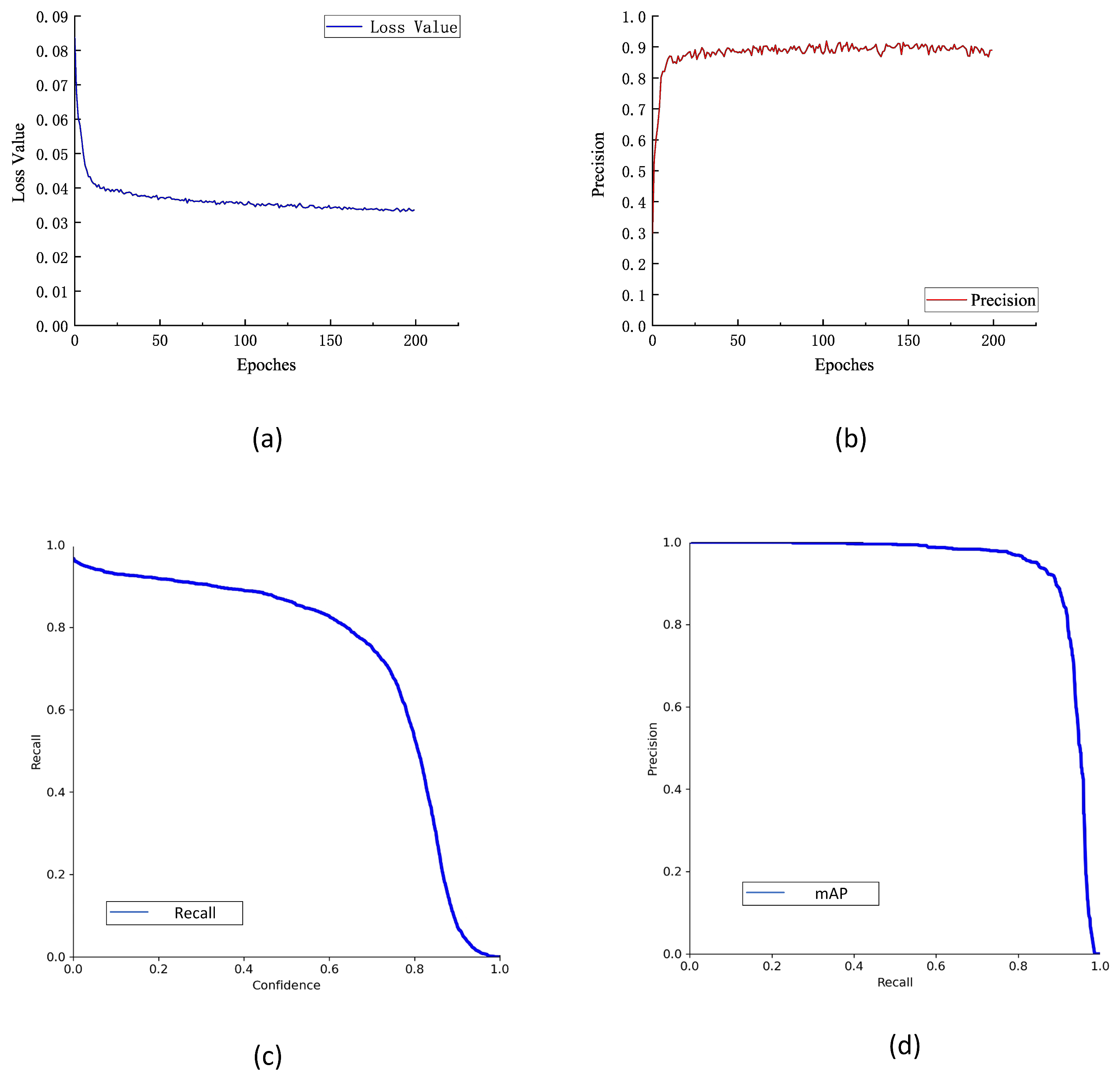
3.1. Training Results

In this study, we obtained relevant results by training the model. Figure 10a illustrates the loss curve during the training process. As observed from this graph, the loss value of YOLOv7-tiny rapidly decreased in the initial 70 epochs and stabilized after 120 epochs, indicating the convergence of the loss curve. Figure 10b depicts the precision curve during the training, showing that the precision curve also leveled off around 200 cycles. Figure 10c and Figure 10d respectively describe the recall curve and mAP curve of the model, further verifying the reliability of the improved model. Therefore, the model after 200 epochs was chosen as the bayberry detection model.

3.2. Comparative Study of Attention Mechanisms

Introducing attention mechanisms to the model can effectively enhance its recognition capability in complex environments.

Table 4. Performance comparison of different attention mechanisms.

Model	Precision (%)	Recall (%)	mAP (/%)
YOLOv7-tiny	83.4	96.3	93.7
+CBAM	85.2	97.0	94.1
+CA	84.1	96.5	93.7
+SA	85.0	97.0	93.9
+SimAM	85.3	97.2	93.8

presents the performance of the model after separately incorporating four attention mechanisms: CBAM, CA, SA, and SimAM. As shown, all four attention mechanisms improved the model in terms of precision and recall, with SimAM producing the most significant improvement, increasing precision and recall by 1.9% and 0.9%, respectively. Regarding mAP, CBAM exhibited the most notable improvement, although SimAM also showed a 0.1% increase. Figure 11 displays the detection results of the four attention mechanisms. As can be seen from this figure, both CBAM and SA have missed detections. According to the experimental results, SimAM demonstrated the best performance, and thus it was adopted in this study.

3.3. Ablation Experiment

To verify the effectiveness of additional modules, PConv, SimAM, and SIoU modules were sequentially introduced for ablation experiments. The “√” mark indicates the adoption of the corresponding improvement strategy.

Table 5. Comparison of ablation results.

SIoU	SimAM	PConv	Precision (%)	Recall (%)	mAP (%)	Model Size (MB)	FLOPs (G)
			83.4	96.3	93.7	11.9	6.58
√			84.8	96.5	93.8	11.9	6.58
	√		85.3	97.2	93.8	11.9	6.58
		√	86.2	97.1	93.3	9.1	4.8
√	√		87.9	97.3	93.9	11.9	6.58
√	√	√	88.1	97.6	93.4	9.0	4.8

presents the experimental data results for different combinations.

When the SIoU or SimAM modules were added, the model’s size or the value of the GLOPs did not increase significantly, but precision, recall, and mAP all improved. Notably, precision showed the most significant improvement, increasing by 1.4% and 1.9%, respectively, demonstrating that SIoU and SimAM can effectively enhance the model’s ability to focus on the target. The introduction of the PConv module reduced model size by 22.3% and GLOPs by 27.1%, although mAP decreased by 0.4%, proving that PConv can reduce the computation of the model while maintaining a certain level of precision. The fifth group of experiments indicated that with the combination of SIoU and SimAM, precision, recall, and mAP further increased to 87.9%, 97.3%, and 93.9%, respectively, compared to the previous single-module improvements. Overall, when the SIoU, SimAM, and PConv modules were introduced simultaneously, the model exhibited optimal overall performance, with precision and recall improving by 4.7% and 1.3%, respectively, and the model size decreasing by 22.4%, relative to the model without additional modules. Thus, the ablation experiments validated the effectiveness of adding these modules.

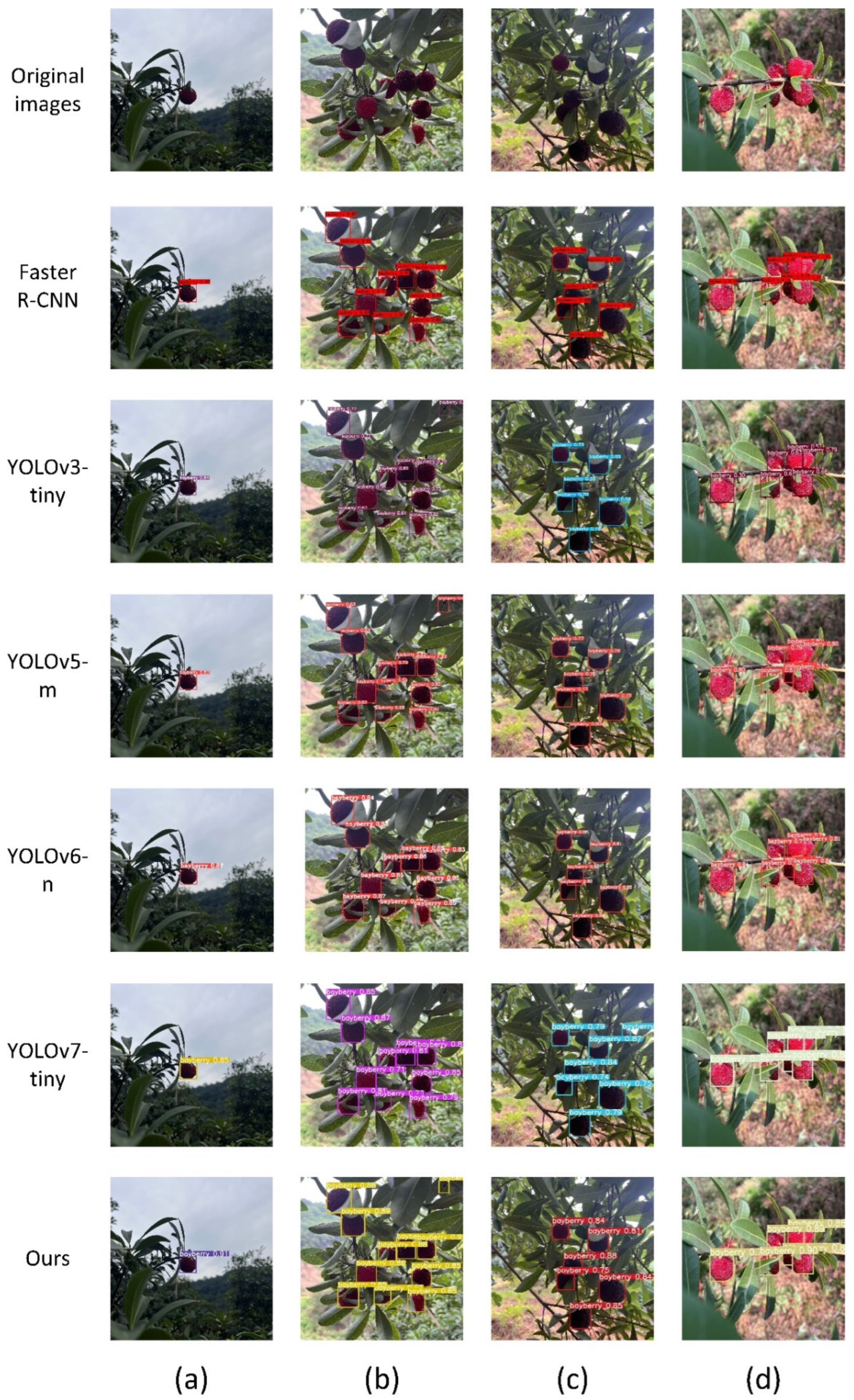
3.4. Comparative Study of Different Networks

To demonstrate the bayberry recognition performance of the proposed model, a comparative experiment was conducted under the same experimental conditions with Faster-RCNN, YOLOv3-tiny, YOLOv5-m, YOLOv6-n, and YOLOv7-tiny, using precision, recall, mAP, and model size as performance indices.

Table 6. Comparison of performance metrics with other network models.

Model	Precision (%)	Recall (%)	mAP (%)	Model Size (MB)
Faster-RCNN	62.1	91.1	90.1	108.7
YOLOv3-tiny	85.4	94.1	87.8	16.9
YOLOv5-m	83.4	97.2	93.9	41.2
YOLOv6-n	81.6	97.1	93.2	10.2
YOLOv7-tiny	83.4	96.3	93.7	11.9
Ours	88.1	97.6	93.4	9.0

provides the comparison results for the six models.

As shown in Figure 12, the improved YOLOv7-tiny achieved 88.1% precision, 97.6% recall, 93.7% mAP, and 9.0 MB model size, indicating favorable results. Compared to the two-stage object detection algorithm Faster R-CNN, precision, recall, and mAP increased by 26.0%, 6.5%, and 3.3%, respectively, while the model size decreased by 99.7 MB. Compared to YOLOv3-tiny, the improvements were 2.7%, 3.5%, and 5.6%, respectively, with a model size reduction of 7.9 MB. Compared to YOLOv5-m, improvements of 4.7%, 0.4%, and 0.5% were observed, with a model size reduction of 32.2 MB. Compared to YOLOv6-n, improvements of 6.5%, 0.5%, and 0.2% were respectively observed, with a model size reduction of 1.2 MB. Compared to the original YOLOv7-tiny, precision and recall increased by 4.7% and 1.3%, respectively, mAP decreased by 0.3%, and model size decreased by 2.9 MB. In summary, the improved YOLOv7-tiny was slightly lower in mAP than the original model, but outperformed the other mainstream models in all other indicators. Therefore, the proposed YOLOv7-tiny model exhibited superior performance in bayberry recognition.

For a more intuitive comparison of the improved model’s performance, images from four common scenes (single fruit, multiple fruits, and backlight and light-facing) were selected for testing on the six models. The results are shown in Figure 13. As shown in Figure 13a, where there was a single fruit, all six models could accurately identify the bayberry; however, the improved YOLOv7-tiny exhibited higher detection confidence than the other models. Figure 13b illustrates that, as the fruit in the upper right corner was obscured by leaves, Faster R-CNN, YOLO-6-n, and the original YOLOv7-tiny missed it, whereas the improved YOLOv7-tiny detected it. In Figure 13c, the original YOLOv7-tiny misidentified leaves as a fruit, resulting in a false positive, whereas the improved YOLOv7-tiny correctly identified all bayberries. In Figure 13d, the improved YOLOv7-tiny provided more accurate detection boxes than the other five models did. Therefore, the comparative images demonstrate that the improved algorithm achieved more precise recognition, confirming its effectiveness.

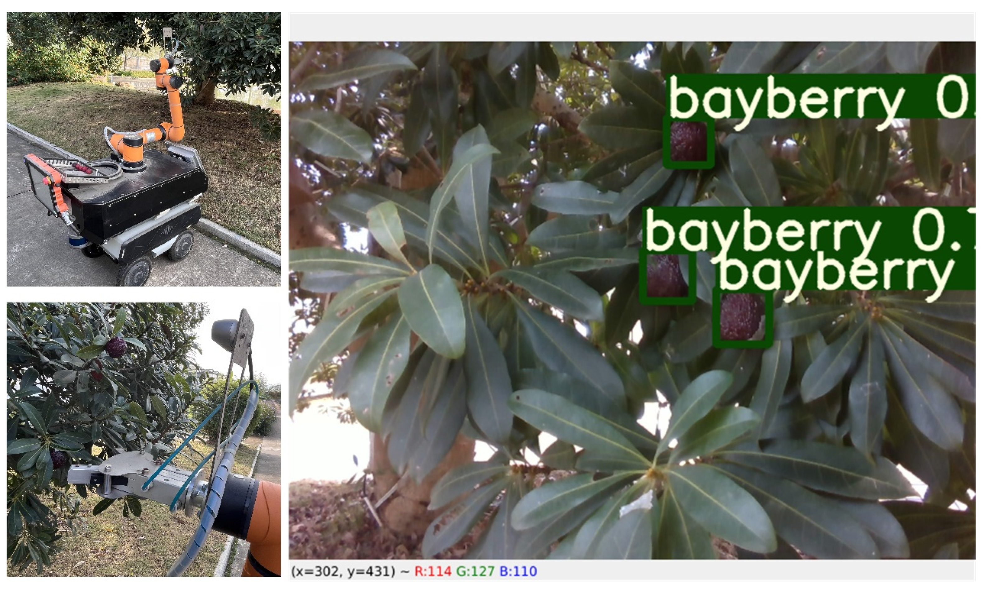
3.5. Harvesting Robot Model Experiment

To further validate whether our improved model can meet the practical requirements of harvesting, we tested it using a harvesting robot in a field experiment. The test site of this experiment is the floriculture forest fruit experimental base in Jinhua Academy of Agricultural Sciences, Zhejiang Province, China. The robot consisted of a mobile chassis, robotic arm, and depth camera. The relevant hardware and platform parameters of the harvesting robot are shown in

Table 7. Hardware and platform parameters for harvesting robots.

Parameter	Value	Parameter	Value
Display Card	Nvidia RTX 1050	System	Ubuntu18.04
Camera	Intel D435	Framework	PyTorch 1.10
Robot Arm	AUBO-i5	Python	3.8
Video Memory	8 G	Image Size	640 × 640

. Firstly the above improved model is deployed to the platform, secondly the depth camera is turned on using control commands, then the detection input is changed to real time video in the model detection module and finally the robotic arm is controlled to locate and harvest the fruits, as depicted in Figure 14. It is evident that the harvesting robot accurately identified all bayberries within the image range. The final experimental results showed that the improved model has a miss detection rate of 4% and an error rate of 3% for bayberries. In addition, the location and size of the recognized bounding box are accurate, and the spatial localization ability of the model meets the requirements and complies with the harvesting standards.

4. Discussion

The traditional method of picking bayberry by hand is no longer suitable for the needs of modern agricultural development due to the increase in labor costs and the low efficiency of picking. Therefore, in recent years, the technology related to picking robots has been continuously developed, which effectively improves the picking efficiency of agricultural fruits, reduces the cost of manual picking, and improves the economic value of agricultural fruits. The visual detection of fruits is a key step for selecting robots to complete the picking task, and the algorithm of fruit detection based on deep learning is better than the traditional detection algorithm in terms of speed and accuracy. Deep learning object detection algorithms can be categorized into two types: two-stage and one-stage. From Table 6, it can be seen that Faster-RCNN, as a two-stage detection algorithm, does not meet the requirements for harvesting recognition either in terms of detection accuracy or model volume. The YOLO algorithm is one of the most popular one-stage detection algorithms. Its simple network structure and high detection speed make it widely applicable for agricultural harvesting robots. YOLOv7 is the latest detection algorithm in the YOLO series, and a lot of improvements have been made to it compared to its predecessor. First, it introduces the Extended Efficient Layer Aggregation Network (E-ELAN). The E-ELAN module strengthens the network’s feature extraction ability by controlling the shortest and longest gradient paths. Second, it introduces reparameterized convolution (RepConv), which employs two different structures during training and inference. In the training phase, it utilizes a multi-branch path structure to enhance network performance, whereas in the inference phase, it adopts a single-path structure derived from reparameterization to boost network inference speed. Finally, YOLOv7 employs a cascade-based model scaling method, allowing the selection of an appropriate model size according to specific task requirements to meet detection demands. Table 6 shows that YOLOv7 has the best overall algorithmic performance compared to previous versions. In this study, we added Partial Convolution (PConv), SimAM Attention Mechanism and SIoU to YOLOv7-tiny to improve the accuracy of poplar plum (Chinese bayberry) detection in the complex environment of the orchard. As can be seen from Figure 13, the improved model effectively solves the phenomena of missed detection, wrong detection, and inaccurate localization of the bounding box produced by the original model

However, this study has certain shortcomings. First, the study only dealt with the identification and harvesting of bayberry fruits without distinguishing whether the fruits were ripe and ready for harvesting. Additionally, the dataset only included bayberry varieties from the region, and data were not collected for other varieties of bayberry. Therefore, future work will include collecting data on the ripeness of bayberries, as well as using other varieties of bayberry to enrich the dataset and make the algorithm more accurate.

5. Conclusions

To precisely detect bayberry fruits in hilly environments, this study first conducted comparative experiments on three versions of YOLOv7 under the same conditions. The results indicated that YOLOv7-tiny outperformed the other two versions in terms of mAP, recall, and model size. Therefore, YOLOv7-tiny was chosen for further experiments. Second, to address the original YOLO algorithm’s suboptimal performance in small object detection, an improved YOLOv7-tiny network model was proposed. The model incorporated PConv, SimAM, and SIoU modules to enhance its efficacy in small object detection. Experimental results demonstrated that the improved model achieved 97.6% recall and 9.0 MB model size. Meanwhile, the precision of the improved model is 88.1%, which is 26%, 2.7%, 4.7%, 6.5%, and 4.7% higher than that of Faster R-CNN, YOLOv3-tiny, YOLOv5-m, YOLOv6-n, and YOLOv7-tiny, respectively. The detection result images revealed that the improved model not only effectively detected highly shaded bayberries but also avoided false positives, thus outperforming the other algorithms. Finally, to validate its feasibility, the improved algorithm was deployed on a harvesting robot for the harvesting experiment. The results demonstrated that the algorithm accurately identified all targets in the bayberry tree images.

In conclusion, this study proposes an algorithm that can efficiently and accurately recognize bayberry. The harvesting robot can detect and localize the location of bayberry fruits in real time by using this algorithm for accurate harvesting, which promotes the development of precision agriculture to a certain extent.

References

1. Zhu, C.; Feng, C.; Li, X.; Xu, C.; Sun, C.; Chen, K. Analysis of expressed sequence tags from Chinese bayberry fruit (Myrica rubra Sieb. and Zucc.) at different ripening stages and their association with fruit quality development. Int. J. Mol. Sci. 2013, 14, 3110–3123. [Google Scholar] [CrossRef] [PubMed]
2. Ge, S.; Wang, L.; Ma, J.; Jiang, S.; Peng, W. Biological analysis on extractives of bayberry fresh flesh by GC–MS. Saudi J. Biol. Sci. 2018, 25, 816–818. [Google Scholar] [CrossRef]
3. Chen, Y.; Xu, H.; Zhang, X.; Gao, P.; Xu, Z.; Huang, X. An object detection method for bayberry trees based on an improved YOLO algorithm. Int. J. Digit. Earth 2023, 16, 781–805. [Google Scholar] [CrossRef]
4. Hoshyarmanesh, H.; Dastgerdi, H.R.; Ghodsi, M.; Khandan, R.; Zareinia, K. Numerical and experimental vibration analysis of olive tree for optimal mechanized harvesting efficiency and productivity. Comput. Electron. Agric. 2017, 132, 34–48. [Google Scholar] [CrossRef]
5. Ni, H.; Zhang, J.; Zhao, N.; Wang, C.; Lv, S.; Ren, F.; Wang, X. Design on the winter jujubes harvesting and sorting device. Appl. Sci. 2019, 9, 5546. [Google Scholar] [CrossRef]
6. Wang, Y.; Wu, H.; Zhu, Z.; Ye, Y.; Qian, M. Continuous picking of yellow peaches with recognition and collision-free path. Comput. Electron. Agric. 2023, 214, 108273. [Google Scholar] [CrossRef]
7. Yang, H.; Chen, L.; Ma, Z.; Chen, M.; Zhong, Y.; Deng, F.; Li, M. Computer vision-based high-quality tea automatic plucking robot using Delta parallel manipulator. Comput. Electron. Agric. 2021, 181, 105946. [Google Scholar] [CrossRef]
8. Lin, G.; Tang, Y.; Zou, X.; Li, J.; Xiong, J. In-field citrus detection and localisation based on RGB-D image analysis. Biosyst. Eng. 2019, 186, 34–44. [Google Scholar] [CrossRef]
9. Wu, G.; Li, B.; Zhu, Q.; Huang, M.; Guo, Y. Using color and 3D geometry features to segment fruit point cloud and improve fruit recognition accuracy. Comput. Electron. Agric. 2020, 174, 105475. [Google Scholar] [CrossRef]
10. Zhang, X.; Zhang, Y.; Gao, T.; Fang, Y.; Chen, T. A novel SSD-based detection algorithm suitable for small object. IEICE Trans. Inf. Syst. 2023, 106, 625–634. [Google Scholar] [CrossRef]
11. Zhang, Z.; Shi, R.; Xing, Z.; Guo, Q.; Zeng, C. Improved faster region-based convolutional neural networks (R-CNN) model based on split attention for the detection of safflower filaments in natural environments. Agronomy 2023, 13, 2596. [Google Scholar] [CrossRef]
12. Li, J.; Chen, J.; Sheng, B.; Li, P.; Yang, P.; Feng, D.D.; Qi, J. Automatic detection and classification system of domestic waste via multimodel cascaded convolutional neural network. IEEE Trans. Ind. Inform. 2022, 18, 163–173. [Google Scholar] [CrossRef]
13. Dai, L.; Sheng, B.; Chen, T.; Wu, Q.; Liu, R.; Cai, C.; Wu, L.; Yang, D.; Hamzah, H.; Liu, Y.; et al. A deep learning system for predicting time to progression of diabetic retinopathy. Nat. Med. 2024, 30, 584–594. [Google Scholar] [CrossRef] [PubMed]
14. Dai, L.; Wu, L.; Li, H.; Cai, C.; Wu, Q.; Kong, H.; Liu, R.; Wang, X.; Hou, X.; Liu, Y.; et al. A deep learning system for detecting diabetic retinopathy across the disease spectrum. Nat. Commun. 2021, 12, 3242. [Google Scholar] [CrossRef]
15. Girshick, R. Fast R-CNN. Fast R-CNN. In Proceedings of the 2015 IEEE International Conference on Computer Vision (ICCV), Santiago, Chile, 7–13 December 2015; pp. 1440–1448. [Google Scholar]
16. Ren, S.; He, K.; Girshick, R.; Sun, J. Faster R-CNN: Towards real-time object detection with region proposal networks. IEEE Trans. Pattern Anal. Mach. Intell. 2017, 39, 1137–1149. [Google Scholar] [CrossRef]
17. He, K.; Gkioxari, G.; Dollár, P.; Girshick, R. Mask R-CNN. In Proceedings of the IEEE International Conference on Computer Vision (ICCV), Venice, Italy, 22–29 October 2017; pp. 2980–2988. [Google Scholar]
18. Yu, Y.; Zhang, K.; Yang, L.; Zhang, D. Fruit detection for strawberry harvesting robot in non-structural environment based on Mask-RCNN. Comput. Electron. Agric. 2019, 163, 104846. [Google Scholar] [CrossRef]
19. Liu, Y.; Ren, H.; Zhang, Z.; Men, F.; Zhang, P.; Wu, D.; Feng, R. Research on multi-cluster green persimmon detection method based on improved Faster RCNN. Front. Plant Sci. 2023, 14, 1177114. [Google Scholar] [CrossRef] [PubMed]
20. Redmon, J.; Divvala, S.; Girshick, R.; Farhadi, A. You only look once: Unified, real-time object detection. Proc. IEEE Comput. Soc. Conf. Comput. Vis. Pattern Recognit. 2016, 2016, 779–788. [Google Scholar]
21. Ji, W.; Gao, X.; Xu, B.; Pan, Y.; Zhang, Z.; Zhao, D. Apple target recognition method in complex environment based on improved YOLOv4. J. Food Process Eng. 2021, 44, e13866. [Google Scholar] [CrossRef]
22. Cao, Z.; Yuan, R. Real-Time detection of mango based on improved YOLOv4. Electronics 2022, 11, 3853. [Google Scholar] [CrossRef]
23. Sun, L.; Hu, G.; Chen, C.; Cai, H.; Li, C.; Zhang, S.; Chen, J. Lightweight apple detection in complex orchards using YOLOV5-PRE. Horticulturae 2022, 8, 1169. [Google Scholar] [CrossRef]
24. Li, T.; Sun, M.; He, Q.; Zhang, G.; Shi, G.; Ding, X.; Lin, S. Tomato recognition and location algorithm based on improved YOLOv5. Comput. Electron. Agric. 2023, 208, 107759. [Google Scholar] [CrossRef]
25. Zhou, J.; Zhang, Y.; Wang, J. RDE-YOLOv7: An improved model based on yolov7 for better performance in detecting dragon fruits. Agronomy 2023, 13, 1042. [Google Scholar] [CrossRef]
26. Chen, J.; Liu, H.; Zhang, Y.; Zhang, D.; Ouyang, H.; Chen, X. A Multiscale lightweight and efficient model based on YOLOv7: Applied to citrus orchard. Plants 2022, 11, 3260. [Google Scholar] [CrossRef] [PubMed]
27. Yu, L.; Qian, M.; Chen, Q.; Sun, F.; Pan, J. An improved YOLOv5 model: Application to mixed impurities detection for walnut kernels. Foods 2023, 12, 624. [Google Scholar] [CrossRef]
28. Wang, C.-Y.; Bochkovskiy, A.; Liao, H.-Y.M. Yolov7: Trainable bag-of-freebies sets new state-of-the-art for real-time object detectors. In Proceedings of the IEEE/CVF Conference on Computer Vision and Pattern Recognition, Vancouver, BC, Canada, 17–24 June 2023; pp. 7464–7475. [Google Scholar]
29. Wang, F.; Lv, C.; Dong, L.; Li, X.; Guo, P.; Zhao, B. Development of effective model for non-destructive detection of defective kiwifruit based on graded lines. Front. Plant Sci. 2023, 14, 1170221. [Google Scholar] [CrossRef]
30. Huang, P.; Wang, S.; Chen, J.; Li, W.; Peng, X. Lightweight model for pavement defect detection based on improved YOLOv7. Sensors 2023, 23, 7112. [Google Scholar] [CrossRef]
31. Chen, J.; Kao, S.H.; He, H.; Zhuo, W.; Wen, S.; Lee, C.H.; Chan, S.H.G. Run, don’t walk: Chasing higher FLOPS for faster neural networks. In Proceedings of the IEEE/CVF conference on Computer Vision and Pattern Recognition, Vancouver, BC, Canada, 17–24 June 2023; pp. 12021–12031. [Google Scholar]
32. Lin, X.; Sun, S.; Huang, W.; Sheng, B.; Li, P.; Feng, D.D. EAPT: Efficient attention pyramid transformer for image processing. IEEE Trans. Multimedia 2023, 25, 50–61. [Google Scholar] [CrossRef]
33. Ma, J.; Lu, A.; Chen, C.; Ma, X.; Ma, Q. YOLOv5-lotus: An efficient object detection method for lotus seedpod in a natural environment. Comput. Electron. Agric. 2023, 206, 107635. [Google Scholar] [CrossRef]
34. Zhang, Q.; Yang, Y. SA-Net: Shuffle attention for deep convolutional neural networks. In Proceedings of the IEEE International Conference on Acoustics, Speech and Signal Processing (ICASSP), Toronto, ON, Canada, 6–11 June 2021; pp. 2235–2239. [Google Scholar]
35. Yang, L.; Zhang, R.-Y.; Li, L.; Xie, X. Simam: A simple, parameter-free attention module for convolutional neural networks. In Proceedings of the International Conference on Machine Learning, PMLR, Virtual Event, 18–24 July 2021; pp. 11863–11874. [Google Scholar]
36. Zheng, Z.; Wang, P.; Liu, W.; Li, J.; Ye, R.; Ren, D. Distance-IoU Loss: Faster and Better Learning for Bounding Box Regression. In Proceedings of the AAAI Conference on Artificial Intelligence, New York, NY, USA, 7–12 February 2020; Volume 34, pp. 12993–13000. [Google Scholar]
37. Gevorgyan, Z. SIoU Loss: More Powerful Learning for Bounding Box Regression. arXiv 2022, arXiv:2205.12740. [Google Scholar]
Figure 1. Partial dataset samples. (a) Single fruit. (b) Multiple fruits. (c) Backlight environment. (d) Light-facing environment.
Agriculture 14 01725 g001
Figure 2. Example of Bayberry label fabrication.
Agriculture 14 01725 g002
Figure 3. Visual analysis of the annotated dataset. (a) Distribution of annotated dataset locations. (b) Distribution of annotated dataset sizes.
Agriculture 14 01725 g003
Figure 4. Flow chart of mosaic data augmentation.
Agriculture 14 01725 g004
Figure 5. Convolution structure diagram. (a) Conventional convolution. (b) Partial convolution.
Agriculture 14 01725 g005
Figure 6. Principles of attention mechanism operation. (a) Channel attention mechanism. (b) Spatial attention mechanism. (c) 3D attention mechanism—SimAM.
Agriculture 14 01725 g006
Figure 7. Angle and distance loss.
Agriculture 14 01725 g007
Figure 8. Detection process of Chinese bayberry using improved YOLOv7-tiny model.
Agriculture 14 01725 g008
Figure 9. Overall structure diagram of improved YOLOv7-tiny model.
Agriculture 14 01725 g009
Figure 10. Training results. (a) Loss curve. (b) Precision curve. (c) Recall curve. (d) mAP curve.
Agriculture 14 01725 g010
Figure 11. Detection results of attention mechanisms. (a) CBAM Attention. (b) CA Attention. (c) SA Attention. (d) SimAM Attention.
Agriculture 14 01725 g011
Figure 12. Performance comparison of different network models.
Agriculture 14 01725 g012
Figure 13. Detection results in different scenes. (a) Single fruit. (b) Multiple fruits. (c) Backlight environment. (d) Light-facing environment.
Agriculture 14 01725 g013
Figure 14. Harvesting robot test.
Agriculture 14 01725 g014