The Influence of Planting Density on the Flowering Pattern and Seed Yield in Peanut (Arachis hypogea L.) Grown in the Northern Region of Japan

Abstract

In peanut cultivation in the Tokachi region of Hokkaido, Japan, it is essential to complete the harvest by early October to prevent frost damage. Therefore, cultivation methods that can accelerate the flowering period are necessary. It is understood that planting density can influence the timing of flowering, with crops often flowering earlier at higher densities. This study aimed to investigate whether growing peanuts at higher densities could advance the flowering period and, consequently, enhance yield. The Japanese peanut variety, Tachimasari, was cultivated in 2022 and 2023 at a conventional planting density of 5.8 plant m⁻² (D5.8) and at density conditions of 8.7 plant m⁻² (D8.7) and 11.6 plant m⁻² (D11.6). The D8.7 and D11.6 plants reached the peak of flowering 2.8 and 5.1 days earlier, respectively, and the end of flowering 3.7 and 8.0 days earlier than the D5.8 plants. Although the total number of flowers was higher in D5.8, pod fertility was greater in D8.7 and D11.6, where plants were able to reduce the occurrence of ineffective flowers and immature pods. Consequently, higher seed yields were observed in D8.7 (2709 kg ha⁻¹) and D11.6 (2754 kg ha⁻¹), where lower individual productivity was offset by higher planting densities, compared to the conventional density condition of D5.8 (2169 kg ha⁻¹).

1. Introduction

With their high content of protein, vitamins, fatty acids, and minerals, peanuts (Arachis hypogea L.) rank among the most significant legumes and are cultivated as a cash crop worldwide. Due to the increasing interest in functional foods, domestic consumption of peanuts in Japan has risen over the past decade, reaching approximately 80,000 tons in 2022 (estimated based on national production and imported products [1]). Peanut production in Japan is concentrated in Chiba Prefecture, which now accounts for over 90% of the country’s domestic peanuts [2]. However, the acreage dedicated to peanut farming in Chiba has been declining, shrinking from 25,000 hectares at its peak in the 1960s to only 5000 hectares in 2023. This reduction is primarily attributed to the aging farmer population and poor yields exacerbated by climate change [2]. The resulting supply shortages and production instability of domestic peanuts have led to price increases and market volatility [3]. To reduce reliance on imported peanuts and ensure a stable supply of domestic peanuts, efforts have been made over the past decade to introduce peanut cultivation to the Tokachi region on the northern island, Hokkaido, which serves as a hub for legume production in Japan [4,5].

The climatic environment of Hokkaido Island falls within the subarctic zone, making it largely unsuitable for cultivating tropical crops such as peanuts. However, the elevated summer temperatures observed in recent years have created favorable conditions for peanut growth, with yields in the Tokachi region often surpassing the Asian average of 263 g m⁻² (weight excluding shells) [1]. Despite this potential, peanut productivity remains inconsistent compared to major temperate crops like wheat and potatoes, with yields varying significantly from year to year. Peanuts are vulnerable to frost, necessitating that farmers complete harvesting and primary drying before the onset of the frost season. In the Tokachi region, damaging frost typically begins in mid-October, although unseasonably early frosts can occur, leading to substantial yield losses. To ensure successful production, the harvest must be completed by the end of September. Many peanut varieties cultivated in the Tokachi region require approximately 40 days from sowing to flowering, followed by an additional 50 days to reach maturity [6,7,8]. Consequently, only flowers that bloom by around August 10 can set seeds by late September. Peanuts with an indeterminate growth habit [9] produce numerous flowers beyond mid-August; however, most of these do not develop into commercially viable pods. These immature pods hinder the efficiency of primary drying post-harvest and deplete nutritional resources from other pods, resulting in reduced pod fertility [10]. Therefore, cultivation methods should be improved to maximize flower production by early August and minimize the occurrence of non-fruiting flowers.

Peanuts exhibit a neutral response to day length and primarily initiate flower bud formation in relation to accumulated temperature [11]. Consequently, the timing of sowing, which influences the accumulation of temperature, can lead to variation in the flowering period. Generally, the earlier the seeds are sown, the sooner they will flower [12]. However, in the Tokachi region, the sowing time for peanuts is fixed in late May due to low temperatures and the risk of late spring frosts prior to that period, as well as labor conflicts with other major crops. Therefore, it is impractical to manipulate the flowering period by altering the sowing time. Conversely, the onset and duration of flowering are influenced by planting density; higher planting densities tend to result in earlier flowering with a shorter duration [11,13,14,15,16]. In peanuts, the flowering period also concludes earlier under high-density conditions because the suppression of lateral branch growth reduces flower bud differentiation during the late growth stage [17]. Conventional peanut cultivation in the Tokachi region employs a planting density of approximately 5.8 plants m⁻² by maintaining 30 cm plant intervals on twin ridges covered with plastic mulch [18]. We hypothesized that cultivating peanuts under denser conditions could accelerate flowering even in this region by increasing competition for space among branches. To date, no studies have examined the impact of planting density on flowering habits in peanut cultivation at high latitudes. Additionally, phenotypic plasticity in flowering habits is known to be more pronounced in procumbent-type peanut varieties compared to erect-type varieties [17]. The varieties predominantly cultivated in the Tokachi region are of the erect type, and it remains unclear whether they can effectively adjust their life history in response to changes in planting density. The objective of this study was to investigate the effects of planting density on the flowering phenology of the Japanese erect-type peanut variety commonly grown in the Tokachi region. Variations in the flowering period may lead to differences in pod productivity; therefore, we also compared the yields of peanuts grown at different planting densities.

2. Materials and Methods

2.1. Culture Condition and Experimental Design

Experiments were conducted over the two consecutive seasons, 2022 and 2023, at the experimental field of Obihiro University of Agriculture and Veterinary Medicine in Obihiro, Hokkaido, Japan (42°52′ N, 143°10′ E, and 77.8 m above sea level). The climate in this region is characterized by an average temperature of 17.9 °C and a cumulative precipitation of 488 mm during the peanut cropping season, which spans from late May to the end of September. In both years, sunflowers were grown as green manure prior to the peanut crop. The soil type in the field was andosol, with a pH range of 6.2 to 6.3. Before planting, the soil contained approximately 7 mg of available nitrogen (including both nitrate and organic forms), 35 mg of available phosphate, and 52 mg of exchangeable potassium per 100 g of soil. To amend the soil, calcium carbonate was applied for soil amendment at a rate of 1000 kg ha⁻¹ before basal fertilization. Subsequently, the soil was fertilized with 19 kg ha⁻¹ of nitrogen (N), 160 kg ha⁻¹ of phosphorus pentoxide (P₂O₅), 83 kg ha⁻¹ of potassium oxide (K₂O), and 29 kg ha⁻¹ of magnesium oxide (MgO), which represent the standard application rates for legume crops in the Tokachi region.

Before planting, the soil in the field was covered with transparent plastic mulch of 0.08 mm thickness to promote warming and control weeds. The erect variety ‘Tachimasari’ was selected for the field experiments. Although it is not a recent variety—having been bred at the Chiba Agricultural Experimental Station in 1974—Tachimasari is noted for its extremely early maturity and achieves the highest yields when cultivated in cooler areas, including the Tokachi region [4,7]. Seeds were hand-sown on May 23 in both years, arranged in two ridges spaced 45 cm apart on the mulch, with three different planting intervals: 30 cm, 20 cm, and 15 cm. These intervals corresponded to planting densities of approximately 5.8 plants m⁻², 8.7 plants m⁻², and 11.6 plants m⁻², respectively. Each plot was designated as D5.8, D8.7, and D11.6 for convenience. D5.8 (30 cm interval) represents the current standard condition for peanut mulch culture in the Tokachi region. The field was organized using a randomized block design, consisting of three plots with different planting densities, each replicated three times per year. Each plot area comprised two ridges 10 m long (approximately 1 m × 10 m). Following bud emergence, cultural practices—including the management of foliar diseases and noxious weeds—were implemented according to conventional management methods in the Tokachi region.

2.2. Counting of Flower Number

The number of newly bloomed flowers was surveyed daily for four randomly chosen plants from a plot, starting from the date of the first bloom until September 15, when bud formation was nearly complete. The cumulative number of flowers was calculated and plotted against the number of days after seed sowing (DAS). The trajectory of the values exhibited a typical sigmoid distribution and was fitted to the Gompertzian function [19], expressed as follows:

$$f(x)=K·a^{e^{-bx}},$$

(1)

where the variable x represents the number of days since seed sowing, and the constant K denotes the upper asymptote, which is the expected final cumulative number of flowers. The constant a is referred to as the location parameter, determining the starting point of the curve, while the constant b serves as a growth-rate coefficient that influences the slope of the curve [20,21]. To determine the inflection point, the first-order differential expression of the function was computed as follows:

$$f^{\prime }(x)=K·\ln a·\ln b·a^{b^x}·b^z.$$

(2)

The inflection point of the curve, which indicates the maximum relative growth rate, is represented as the local maximum of the first-order differential expression and is equivalent to K/e. At this point, ∆f(x) signifies the maximum number of flowers that bloom in a single day. Consequently, the date corresponding to the inflection point was designated as the “peak of flowering (PF)”. Gompertzian functions essentially consist of two distinct phases surrounding the inflection point. During these phases, the relative growth rate of the dependent variable initially increases according to the function of b, followed by an exponential decline over time. The first and second inflection points of the first-order differential expression curve mark the moments when the asymptote of the original Gompertzian function experiences a sharp increase and subsequent decline, respectively, in the aforementioned phases. As a result, the dates corresponding to the first and second inflection points of the first-order differential expression curve are identified as the “inception of flowering (IF)” and “termination of flowering (TF)”, respectively. The duration between the IF and TF can be regarded as the significant flowering period.

2.3. Yield Measurement

Plants used for the flowering survey were harvested all together on 25 September in 2022, and 20 September in 2023, respectively. The number of pegs, fertile pods, and total pods were recorded for each plant. Subsequently, the pod setting rate and pod fertility were calculated by dividing the total number of pods by the number of pegs and the number of fertile pods by the total number of pods, respectively. In this study, a pod was defined as a peg tip that enlarged to at least 1 cm, and a pod containing at least one mature seed was considered fertile. The weight of intact mature seeds was measured for each plant, and the 100-seed weight was calculated based on the number of seeds weighed. On the same day, 20 medium-sized plants were randomly selected from each plot to harvest the pods from the ground. After drying the pods in the sun to approximately 20% moisture content, the mature seeds within the pods were collected to determine the grain yield.

2.4. Statistical Analysis

All data obtained from plant measurements were analyzed using a two-way analysis of variance (ANOVA), with year and planting density as the main variable factors. In the absence of interaction or random block effects, the variances were combined with the total error variance, and the effects of the main factors were re-evaluated. When significant effects of the main factors were identified, a Bonferroni post hoc comparison test at a 5% significance level was conducted to compare the means between years or planting densities. Prior to the analysis, an arcsine transformation was applied to the data for pod setting rate and pod fertility to ensure a normal distribution and equal variance. The software package STATA ver. 17^TM (Lightstone, New York, NY, USA) was used for the analyses.

3. Results

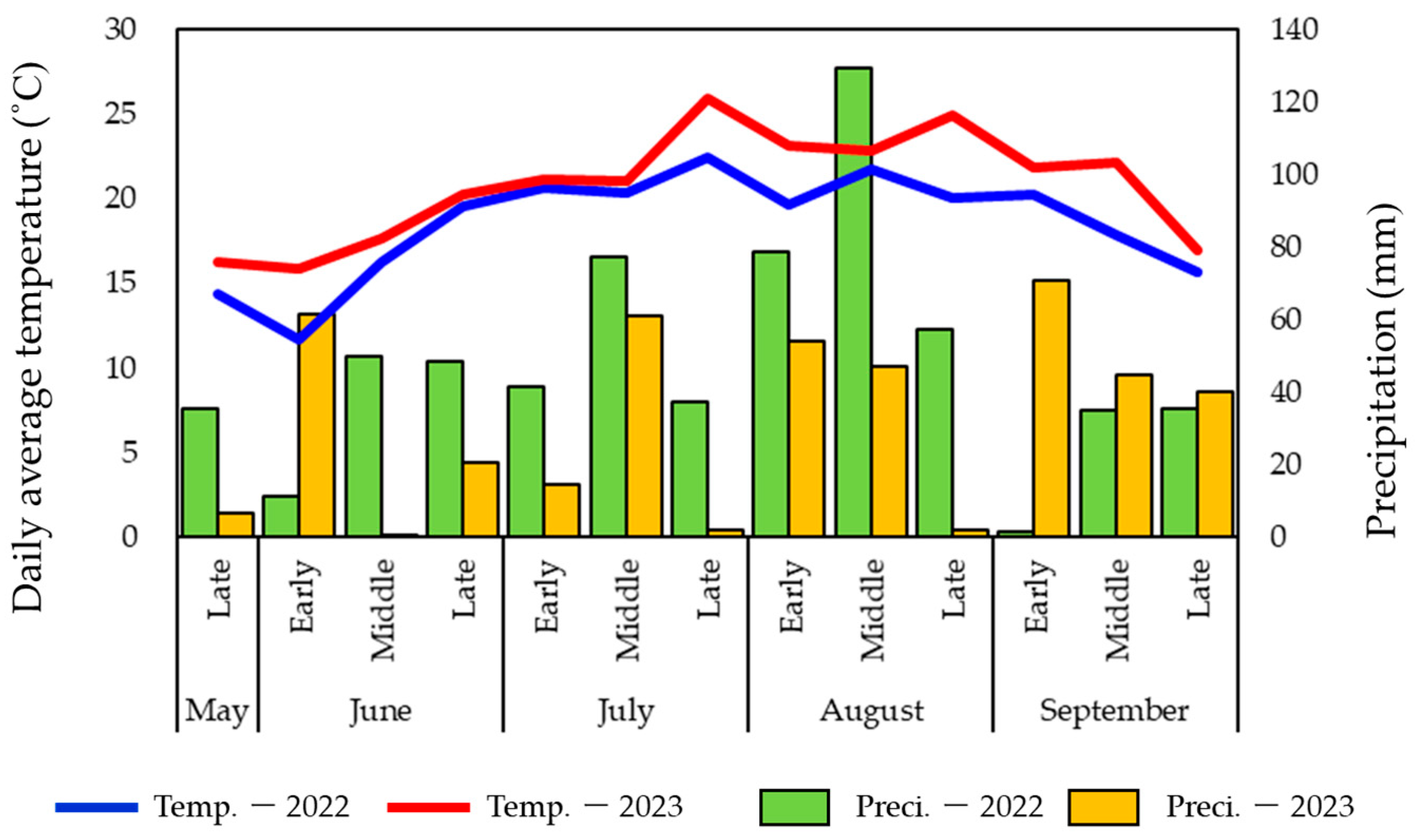
3.1. Weather Conditions of Two Years

The climate data at the experimental field were collected using a data logger (ATOMOS41/ZL6^TM, METER Group, Pullman, WA, USA) during two growing seasons of peanuts (Figure 1). In the initial growth stage of peanuts, the weather in 2023 was warmer and drier compared to 2022. The daily average temperature, cumulative temperature, and cumulative precipitation from the sowing date to the end of June (just before the onset of flowering) were 15.5 °C, 574.0 °C, and 145.5 mm in 2022, and 17.9 °C, 662.3 °C, and 89.0 mm in 2023, respectively. From late July, when pegs and pods began to develop, until harvest, the weather in 2023 was also characterized by higher temperatures and lower precipitation compared to 2022. The daily average temperature, cumulative temperature, and cumulative precipitation during this period (July 21 to September 30) were 19.7 °C, 1419.3 °C, and 375.0 mm in 2022, and 22.5 °C, 1628.7 °C, and 261.0 mm in 2023, respectively. Throughout both years, there were no significant environmental issues that adversely affected peanut growth.

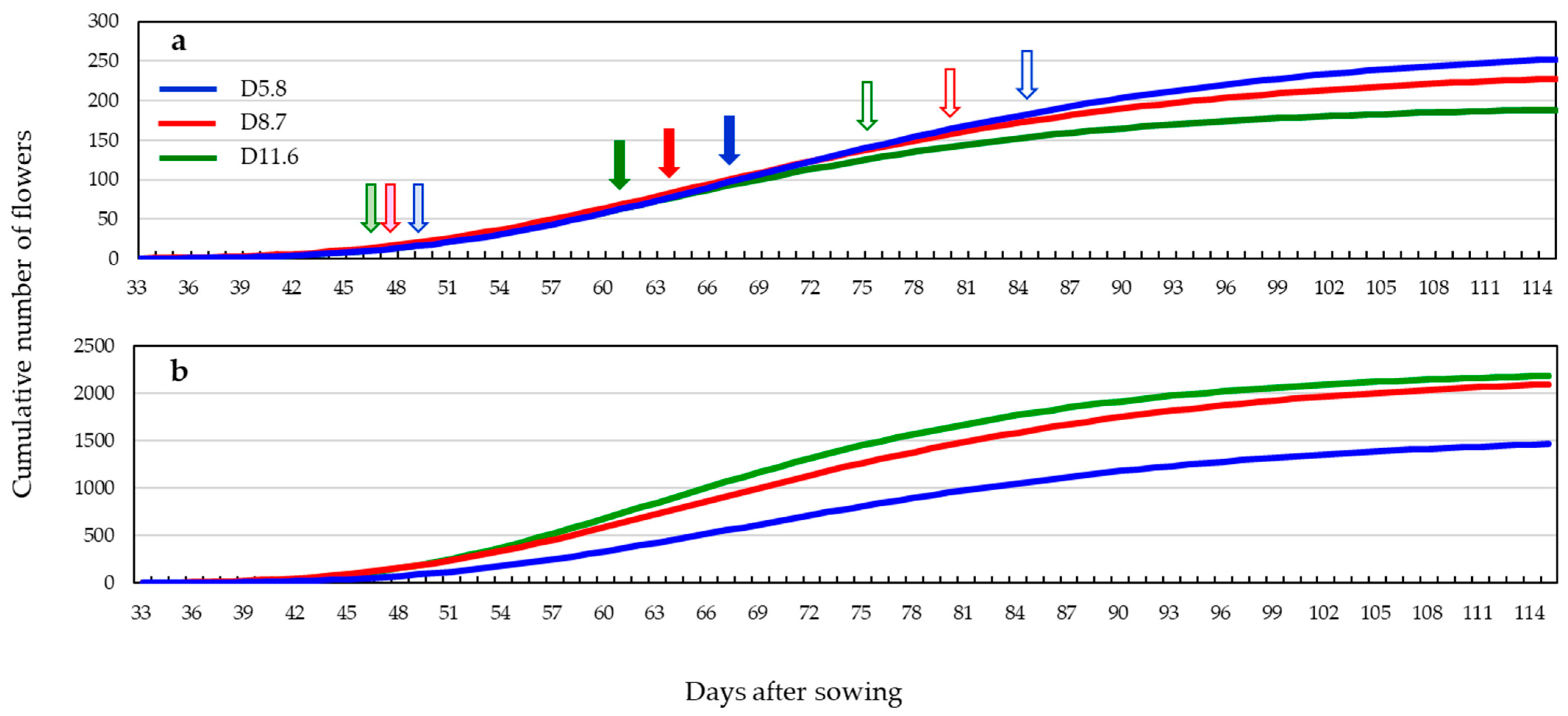
3.2. Flowering Pattern

The flowering process commenced uniformly across the three experimental plots each year, occurring on June 28 (36 DAS) in 2022 and June 25 (33 DAS) in 2023. The actual cumulative number of flowers per plant exhibited similar trajectories in both years, indicating that plants in sparse conditions tended to produce more flowers (Figure S1). As no interactions between year and planting density were detected, the data from 2022 and 2023 were combined into a single dataset for further analysis. The trajectories of the graph elements were fitted to the Gompertzian function to determine the mathematical parameters (Figure 2a,

Table 1. The maximum daily flowering number (∆f(x)) and flowering schedule of the plants in the three experimental plots estimated from the Gompertzian functions.

	Gompertzian Parameters			Maximum	Days after Sowing			Flowering Period
Plot	K	a	b	∆f(x)	IF	PF	TF	(Days)
D5.8	270.8	33.0	0.056	5.6	49.1	66.7	84.2	35.1
D8.7	241.3	33.1	0.057	5.1	47.2	63.9	80.5	33.3
D11.6	194.4	33.0	0.066	4.7	46.8	61.6	76.2	29.4

K: the expected final cumulative number of flowers; a: the location parameter determining the starting point of the curve; b: the growth-rate coefficient affecting the slope of the curve; ∆f(x): the number of flowers newly bloomed in one day; IF: the number of days for the inception of flowering; PF: the number of days for the peak of flowering; TF: the number of days for the termination of flowering.

). The expected final cumulative number of flowers, denoted as K, was higher in plots with a lower planting density; specifically, the value of 270.8 flowers per plant in D5.8 was approximately 1.4 times greater than the 184.4 flowers per plant in D11.6. The maximum number of flowers produced per day also followed the order of D5.8 (5.6 flowers per plant per day), D8.7 (5.1 flowers per plant per day), and D11.6 (4.7 flowers per plant per day). The actual daily flower counts in the three plots are illustrated in Figure S2. The days to IF did not reach a difference of two days among the plots, ranging from 46.8 DAS in D11.6 to 48.1 DAS in D5.8. However, as growth progressed, differences in the flowering stage became apparent among the plots, with D11.6 reaching PF 5.1 days earlier than D5.8. The D11.6 plants ceased practical flowering at 76.2 DAS, which was approximately 3.7 days and 8.0 days earlier than the D8.7 and D5.8 plants, respectively. Consequently, the flowering period, determined from the duration between IF and TF, was shorter in plots with higher planting densities. Although flower productivity was lower in plots with higher planting density, the number of flowers per area, calculated as the product of the number of flowers per plant and planting density, was greater in the densely planted plots (Figure 2b). Notably, significantly more flowers were counted throughout the observation period in D11.6 and D8.7 compared to D5.8, with the final cumulative number of flowers estimated at 2139 and 2012 flowers m⁻² in D11.6 and D8.7, respectively, while D5.8 yielded a lower total of 1570 flowers m⁻².

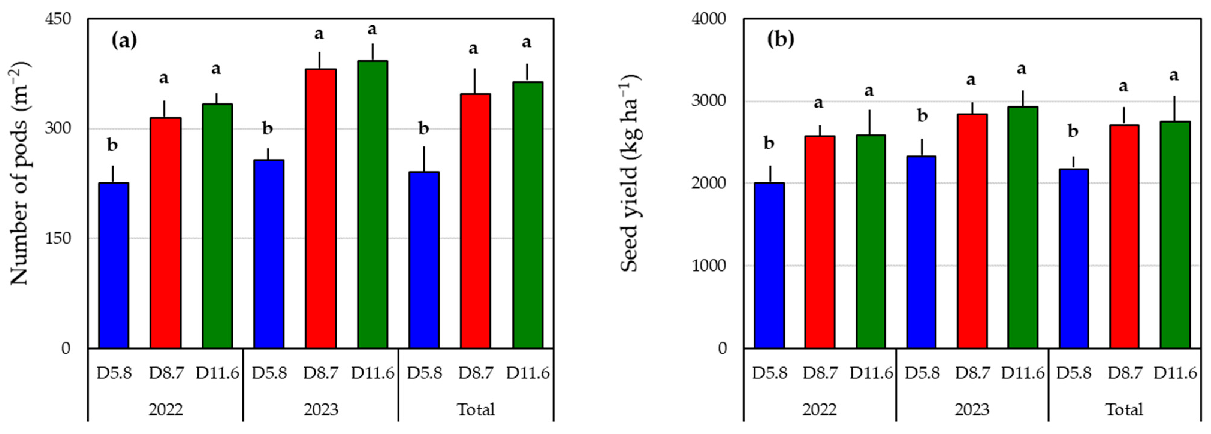
3.3. Seed Yield and Yield Components

ANOVA revealed no interactions between year and planting density in the production of pegs and pods. The planting density appeared to exert a consistent impact on both pegs and pods in 2022 and 2023 (

Table 2. Yield components measured on an individual basis in three plots at different planting densities. Values represent average ± standard error.

		No. of	No. of	No. of	Pod Setting	Pod	100-Seed
Year	Plot	Pegs	Pods	Fertile Pods	Rate (%)	Fertility (%)	Weight (g)
	D5.8	155.0 ± 3.7 a	91.7 ± 3.3 a	52.1 ± 2.7 a	59.5 ± 2.6 a	56.6 ± 1.5 b	47.3 ± 1.2
2022	D8.7	117.2 ± 5.7 b	59.8 ± 3.2 b	40.5 ± 2.2 b	52.0 ± 3.0 b	67.8 ± 0.8 a	48.6 ± 1.1
	D11.6	87.8 ± 4.0 c	41.3 ± 2.3 c	28.8 ± 1.7 c	48.0 ± 3.2 c	69.8 ± 1.7 a	47.6 ± 1.7
	D5.8	147.8 ± 7.6 a	94.7 ± 1.8 a	58.5 ± 2.6 a	65.7 ± 3.2 a	61.8 ± 2.5 b	52.3 ± 1.8
2023	D8.7	112.9 ± 5.7 b	66.3 ± 2.4 b	48.9 ± 3.1 b	59.3 ± 1.6 b	734. ± 2.5 a	52.8 ± 2.0
	D11.6	93.3 ± 3.9 c	54.6 ± 2.6 c	39.7 ± 2.2 c	59.1 ± 2.8 b	72.6 ± 1.4 a	53.4 ± 2.8
	D5.8	151.4 ± 4.2 a	93.2 ± 1.9 a	55.3 ± 1.9 a	62.6 ± 2.1 a	59.2 ± 1.5 b	49.8 ± 1.2
Total	D8.7	115.0 ± 4.0 b	63.0 ± 2.1 b	44.7 ± 2.0 b	55.7 ± 1.8 b	70.6 ± 1.4 a	50.7 ± 1.2
	D11.6	90.6 ± 2.8 c	48.0 ± 2.2 c	34.3 ± 1.8 c	53.5 ± 2.4 c	71.2 ± 1.1 a	50.5 ± 1.7
ANOVA	Year	*	**	**	**	**	**
	Density	**	**	**	**	**	ns
Year × Density		ns	ns	ns	ns	ns	ns

Values followed by different letters within columns of same year are significantly different at p = 0.05 according to Bonferroni post hoc comparison test. ns = not-significant, * = significant at p = 0.05, ** = significant at p = 0.01.

). As planting density increased by the order of 5.8, 8.7, and 11.6, the number of pegs and pods produced per plant significantly decreased at harvest time. The average number of pegs and total pods per plant at D11.6 were 90.6 ± 2.8 and 48.0 ± 2.2 over the two years, respectively, which represented approximately 60% and 50% of those at D5.8 (151.4 ± 4.2 and 93.2 ± 1.9, respectively). The pod setting rate was also strongly influenced by planting density, being significantly higher, in the order of D5.8 (62.6 ± 2.1%), D8.7 (55.7 ± 1.8%), and D11.6 (53.5 ± 2.4%). The D5.8 plants produced significantly more fertile pods than those in the other plots, while pod fertility was relatively higher in D8.7 (70.6 ± 1.4%) and D11.6 (71.2 ± 1.1%) compared to D5.8 (59.2 ± 1.5%). There was no effect of planting density on 100-seed weight, which averaged from 49.8 ± 1.2 g (D5.8) to 50.7 ± 1.2 g (D8.7) over the two years (Table 2).

The number of fertile pods produced per square meter at D8.7 and D11.6 was significantly higher than at D5.8 in both 2022 and 2023 (Figure 3a). The average number of fertile pods at D8.7 and D11.6 was 347.5 ± 25.7 pods per square meter and 362.9 ± 15.3 pods per square meter over the two years, respectively, both of which are approximately 1.5 times greater than the average at D5.8 (241.1 ± 22.2 pods per square meter). Plant pod productivity was lower in plots with higher planting density; however, the number of fertile pods per area was compensated by the number of plants, resulting in a tendency for higher pod counts in the densely planted plots. Consequently, seed yields were also significantly greater at D8.7 and D11.6 compared to D5.8 (Figure 3b). The average seed yield over the two years at D8.7 and D11.6 reached 2709 ± 76 kg ha⁻¹ and 2754 ± 82 kg ha⁻¹, respectively, both of which are approximately 1.3 times the yield at D5.8 (2169 ± 38 kg ha⁻¹).

4. Discussion

The growth of individual plants varies with planting density, with those grown at lower densities generally exhibiting greater biomass [22,23,24,25]. This phenomenon occurs because each plant can access more resources, such as light and soil nutrients, in a less crowded environment compared to a denser one [16,26,27]. Previous studies on peanuts have also confirmed that a wider row or plant spacing results in larger plant size [18,28,29,30]. Although this study did not specify plant size at harvest, our previous research on the same set of peanut plants as this study, namely Tachimasari grown at varying planting densities ranging from 5.8 plants m⁻² to 11.7 plants m⁻², indicated that plant size decreased as density increased [18].

Planting density significantly affects plant size, which ultimately determines the number of flowers produced. Increased spacing has been shown to promote the development of more primary and secondary branches in statice (Limonium sinuatum) [25], safflower (Carthamus tinctorius) [31], and potatoes [32], resulting in a higher final flower count per plant. A similar trend of larger plants at lower densities producing more branches and flowers was also reported in Tachimasari [18]. Due to their indeterminate growth habit, peanuts in sparser environments can continue to develop branches and differentiate flower buds until late in the growth stage. Well-branched, larger plants in D5.8 were estimated to produce 75 more flowers than smaller plants in D11.6 over the growing season (K in Table 1). The flexible variation in flower number with planting density observed in the Argentine procumbent-type variety [17] was also noted in the Japanese erect-type variety. Furthermore, planting density significantly influences flowering patterns. For instance, in rice, narrowing the row arrangement at transplanting decreased the days to panicle emergence [33,34], potentially leading to earlier flowering. Similar effects of reduced days to flowering due to increased planting density have been observed in crops such as tomato [16], sunflower [13], canola [15], and wheat [14]. However, a contrasting trend of delayed flowering under dense conditions was reported for some crops in a review by Postma et al. [27]. In Tachimasari, the effect of planting density on the days to the onset of flowering was not different largely, with plants in plots of varying densities entering the flowering phase on nearly the same date. This highlights the characteristics of peanuts as a neutral plant that primarily initiates flower bud formation principally in response to accumulated temperature and the number of mature leaves, rather than body size determined by planting density [11,35,36]. Conversely, flowering duration in Tachimasari was greatly influenced by planting density, being shorter under higher density conditions. Canola [37], maize [38], and the ephemeral wild herb Cardamine hirsute [39] exhibited a similar relationship between planting density and flowering duration, with plants in high-density stands terminating flowering significantly earlier. The mechanism by which these plants terminate flowering earlier under high-density conditions is not well understood; however, it is likely that in peanuts, with their indeterminate growth habit, competition with surrounding plants in high-density stands hinders branch development in the later growth stage, resulting in the earlier termination of flower bud formation compared to low-density stands [25,37].

The flowers that contribute to peanut production in the Tokachi region are those that have bloomed by approximately August 10. The cumulative number of flowers per plant on August 10 in D5.8, estimated using the Gompertzian function (Figure 2), averaged 162 flowers per plant on average over the two-year period, which accounted for less than 60% of the expected final cumulative flower count. In D8.7 and D11.6, where the peak flowering period had been advanced, 160 and 143 flowers per plant had bloomed by this date, corresponding to approximately 70% of the anticipated final cumulative flower count. Despite the higher flower productivity of the D5.8 plants, the cumulative number of flowers as of August 10 showed only slight variation among the three experimental plots. This resulted in a greater number of flowers per area in the plots with higher planting densities, with 1420 and 1600 flowers m⁻² in D8.7 and D11.6, respectively, compared to 930 flowers m⁻² in D5.8, on August 10.

Higher pod fertility observed at D8.7 and D11.6 may be attributed to the high-density planting, which induces earlier flowering. This phenomenon can help reduce the likelihood of frost damage and the occurrence of unfruitful flowers [9,10,11,17,18]. Additionally, it indicates fewer immature pods, which are more susceptible to rot and can interfere with post-harvest drying operations, at D8.7 and D11.6 compared to D5.8 [10]. Conversely, the pod setting rate decreased as the planting density increased. The abscission of flowers and fruits is believed to occur when the source size is small relative to the sink size, resulting in insufficient nutrient resources being supplied to the reproductive parts [34,40]. It is posited that the Tachimasari, which exhibited a smaller body size in the densely planted plots, could not allocate adequate resources to reproduction during the later growth stages. Consequently, the lower pod setting rate may also contribute to the reduced number of immature pods in these densely planted plots.

Density is a critical regulatory factor that influences the yields of grains and legumes, as productivity is determined by the performance of individual plants and the number of plants per unit area. Peanut plants, particularly procumbent varieties, exhibit a greater pod set as planting density decreases [18,30]. A similar trend was observed in the erect variety Tachimasari, where the number of pods produced by a plant under conventional planting density conditions in the Tokachi region (D5.8) was 1.5 to 2 times greater than that produced under 1.5 to 2 times denser conditions (D8.7 and D11.6), respectively. However, regarding fertile pods, which significantly contribute to yield, the number produced by the D5.8 plants was only 1.2 times and 1.6 times greater than that produced by the D8.7 and D11.6 plants, respectively. Although prolonged flowering in D5.8 increased the total number of pods, it did not necessarily result in higher seed production. Consequently, seed yields were higher in D8.7 and D11.6, where the increased planting density compensated for the lower individual plant performance, compared to D5.8.

5. Conclusions

The erect-type peanut variety Tachimasari exhibited a change in its growth pattern in response to varying planting densities. In environments with higher planting densities, the plants tended to terminate flowering earlier, which resulted in a reduction in ineffective flowers and immature pods. Although individual productivity decreased, the yields at densities of 8.7 and 11.6 plants m⁻² were approximately 1.5 times higher than those at the conventional density of 5.8 plants m⁻². This study found that yield could be enhanced by planting at a higher density compared to conventional conditions and by advancing the flowering period. Although there was no significant difference in yield, a planting density of 8.7 plants m⁻² is considered the optimal choice among the conditions established in this study, particularly when factoring in the cost of seeds for sowing.

References

1. FAOSTAT. Available online: https://www.fao.org/faostat/en/#data/QCL (accessed on 2 July 2024).
2. Official Statistics of Japan. Available online: https://www.e-stat.go.jp/en/stat-search/files?page=1&layout=datalist&toukei=00500215&tstat=000001013427&cycle=0&tclass1=000001032288&tclass2=000001034728&tclass3val=0 (accessed on 24 June 2024).
3. Nojima, N. Economic globalization and management strategies for the peanut processing industry. J. Comput. Soc. Sci. 2012, 10, 11–24. [Google Scholar]
4. Akimoto, M.; Sato, K.; Kumada, F.; Tsujimoto, H.; Kobayashi, N.; Hirato, S.; Tanaka, I. Basic study for the appropriate cultivation method of groundnut (Arachis hypogaea L.) in the Tokachi region II. Selection of the suitable varieties for the production in the Tokachi region. Res. Bull. Obihiro Univ. 2018, 39, 15–23. [Google Scholar]
5. Akimoto, M.; Nakata, S.; Kumada, F.; Tsujimoto, H.; Kobayashi, N.; Hirato, S.; Tanaka, I. Basic study for the appropriate cultivation method of groundnut (Arachis hypogaea L.) in the Tokachi region. Res. Bull. Obihiro Univ. 2017, 38, 13–24. [Google Scholar]
6. Takahashi, Y.; Takeuchi, S.; Kamekura, H.; Saito, S.; Ishii, R.; Ishida, Y.; Nagasawa, J.; Katsura, H. On the new peanut variety “Nakateyutaka”. Bull. Chiba Agric. Exp. Stn. 1981, 22, 57–69. [Google Scholar]
7. Takeuchi, S.; Kamekura, H.; Saito, S.; Ishii, R.; Ishida, Y. On the new peanut variety “Tachimasari”. Bull. Chiba Agric. Exp. Stn. 1975, 16, 135–146. [Google Scholar]
8. Suzuki, K.; Nakanishi, T.; Takahashi, Y.; Matsuda, T.; Iwata, Y.; Suzuki, S.; Ishii, R.; Kajiro, M.; Katsura, H.; Yashiki, T. On ’Satonoka’. a new variety of peanut (Arachis hypogaea L.). Bull. Chiba Agric. Exp. Stn. 1997, 38, 55–66. [Google Scholar]
9. Liew, X.Y.; Sinniah, U.R.; Yusoff, M.M.; Witty, U.A. Flowering pattern and seed development in ideterminate peanut cv. ‘Margenta’ and its influence on seed quality. Seed Sci. Technol. 2021, 49, 45–62. [Google Scholar] [CrossRef]
10. Stalker, H.T. Peanut (Arachis hypogaea L). Field Crops Res. 1997, 53, 205–217. [Google Scholar] [CrossRef]
11. Cattan, P.; Fleury, A. Flower production and growth in groundnut plants. Eur. J. Agron. 1998, 8, 13–27. [Google Scholar] [CrossRef]
12. Jonishi, T.; Fujii, Y.; Nakamura, C.; Omichi, M. Effect of sowing date on growth and yield of peanuts (Arachis hypogaea L.) in Hokkaido. Res. Bull. Takushoku Jr. Univ. 2023, 3, 1–8. [Google Scholar] [CrossRef]
13. Demir, İ. Inter and intra row competition effects on growth and yield components of sunflower (Helianthus annuus L.) under rainfed conditions. J. Anim. Plant Sci. 2020, 30, 147–153. [Google Scholar]
14. Geleta, B.; Atak, M.; Baenziger, P.S.; Nelson, L.A.; Baltenesperger, D.D.; Eskridge, K.M.; Shipman, M.J.; Shelton, D.R. Seeding rate and genotype effect on agronomic performance and end-use quality of winter wheat. Crop Sci. 2002, 42, 827–832. [Google Scholar] [CrossRef]
15. Harker, K.N.; O’Donovan, J.T.; Smith, E.G.; Johnson, E.N.; Peng, G.; Willenborg, C.J.; Gulden, R.H.; Mohr, R.; Gill, K.S.; Grenkow, L.A. Seed size and seeding rate effects on canola emergence, development, yield and seed weight. Can. J. Plant Sci. 2015, 95, 1–8. [Google Scholar] [CrossRef]
16. Ismail, S.M.; Mousa, M.A.A. Optimizing tomato productivity and water use efficiency using water regimes, plant density and row spacing under arid land conditions. Irrig. Drain. 2014, 63, 640–650. [Google Scholar] [CrossRef]
17. Haro, R.J.; Carrega, W.C.; Otegui, M.E. Row spacing and growth habit in peanut crops: Effects on seed yield determination across environments. Field Crops Res. 2022, 275, 108363. [Google Scholar] [CrossRef]
18. Sato, S.; Ishiyama, S.; Tanaka, I.; Akimoto, M. Study on the optimal planting density for the cultivation of peanut in Tokachi Region. Jpn. J. Crop Sci. 2024, 93, 122–131. [Google Scholar] [CrossRef]
19. Domínguez-May, R.; Gasca-Leyva, E.; Robledo, D. Harvesting time optimization and risk analysis for the mariculture of Kappaphycus alvarezii (Rhodophyta). Rev. Aquac. 2017, 9, 227–237. [Google Scholar] [CrossRef]
20. Tjørve, K.M.C.; Tjørve, E. The use of Gompertz models in growth analyses, and new Gompertz-model approach: An addition to the Unified-Richards family. PLoS ONE 2017, 12, e0178691. [Google Scholar] [CrossRef]
21. Oshima, K.; Hofuku, I.; Inagawa, A. Two-step cumulative curve and modified Gompertz curve. Jpn. J. Ind. Appl. Math. 1994, 4, 259–274. [Google Scholar] [CrossRef]
22. Isobe, K.; Sato, R.; Sakamoto, S.; Arai, T.; Miyamoto, M.; Higo, M.; Torigoe, Y. Studies on optimum planting density of quinoa (Chenopodium quinoa Willd.) Variety NL-6 considering efficiency for light energy utilization, matter production and yield. Jpn. J. Crop Sci. 2015, 84, 369–377. [Google Scholar] [CrossRef]
23. Jain, R.; Singh, M.K.; Swaroop, K.; Reddy, M.V.; Janakiram, T.; Kumar, P.; Pinder, R. Optimization of spacing and nitrogen dose for growth and flowering of statice (Limonium sinuatum). Indian J. Agric. Sci. 2018, 88, 1108–1114. [Google Scholar] [CrossRef]
24. Bezu, T.; Kassa, N. Planting density and corm size effects on flower yield and quality of cut-freesia (Freesia hybrid) in Ethiopia. J. Appl. Hortic. 2014, 16, 76–79. [Google Scholar] [CrossRef]
25. Barišić, N.; Stojković, B.; Tarasjev, A. Plastic responses to light intensity and planting density in three Lamium species. Plant Syst. Evol. 2006, 262, 25–36. [Google Scholar] [CrossRef]
26. Donald, C.M. Competition among crop and pasture plants. Adv. Agron. 1963, 15, 1–118. [Google Scholar] [CrossRef]
27. Postma, J.A.; Hecht, V.L.; Hikosaka, K.; Nord, E.A.; Pons, T.L.; Poorter, H. Dividing the pie: A quantitative review on plant density responses. Plant Cell Environ. 2021, 44, 1072–1094. [Google Scholar] [CrossRef]
28. Minh, T.X.; Thanh, N.C.; Thin, T.H.; Tieng, N.T.; Giang, N.T.H. Effects of plant density and row spacing on yield and yield components of peanut (Arachis hypogaea L.) on the coastal sandy land area in Nghe An Province, Vietnam. Indian J. Agric. Res. 2021, 55, 468–472. [Google Scholar] [CrossRef]
29. Kharel, P.; Devkota, P.; Macdonald, G.E.; Tillman, B.L.; Mulvaney, M.J. Influence of planting date, row spacing, and reduced herbicide inputs on peanut canopy and sicklepod growth. Agron. J. 2022, 114, 717–726. [Google Scholar] [CrossRef]
30. Cordeiro, C.F.D.S.; Pilon, C.; Echer, F.R.; Albas, R.; Tubbs, R.S.; Harris, G.H.; Rosolem, C.A. Adjusting peanut plant density and potassium fertilization for different production environments. Agron. J. 2023, 115, 817–832. [Google Scholar] [CrossRef]
31. Steberl, K.; Hartung, J.; Munz, S.; Graeff-Hönninger, S. Effect of row spacing, sowing density, and harvest time on floret yield and yield components of two safflower cultivars grown in southwestern Germany. Agronomy 2020, 10, 664. [Google Scholar] [CrossRef]
32. Almekinders, C.J.M. Effect of plant density on the inflorescence production of stems and the distribution of flower production in potato. Potato Res. 1993, 36, 97–105. [Google Scholar] [CrossRef]
33. Hayashi, S. Growth, grain yield and grain quality of sparsely planted rice (Oryza sativa L.) cultivar “Nanatsuboshi” in Hokkaido. Jpn. J. Crop Sci. 2017, 86, 129–138. [Google Scholar] [CrossRef]
34. Hu, Q.; Jiang, W.Q.; Qiu, S.; Xing, Z.P.; Hu, Y.J.; Guo, B.W.; Liu, G.D.; Gao, H.; Zhang, H.C.; Wei, H.Y. Effect of wide-narrow row arrangement in mechanical pot-seedling transplanting and plant density on yield formation and grain quality of japonica rice. J. Integr. Agric. 2020, 19, 1197–1214. [Google Scholar] [CrossRef]
35. Takeuchi, S.; Ashiya, O.; Kamekura, H. On the flowering and fruiting habits of peanut “Chiba Handachi”. Bull. Chiba Agric. Exp. Stn. 1964, 5, 113–121. [Google Scholar]
36. Inoue, Y. Studies on the flowering habit in peanut (Arachis hypogaea L.). Jpn. J. Hortic. 1958, 27, 245–248. [Google Scholar] [CrossRef]
37. Gan, Y.; Harker, K.N.; Kutcher, H.R.; Gulden, R.H.; Irvine, B.; May, W.E.; O’Donovan, J.T. Canola seed yield and phenological responses to plant density. Can. J. Plant Sci. 2016, 96, 151–159. [Google Scholar] [CrossRef]
38. Chassaigne-Ricciulli, A.A.; Mendoza-Onofre, L.E.; Córdova-Téllez, L.; Carballo-Carballo, A.; San Vicente-García, F.M.; Dhliwayo, T. Effective seed yield and flowering synchrony of parents of cimmyt three-way-cross tropical maize hybrids. Agriculture 2021, 11, 161. [Google Scholar] [CrossRef]
39. Cao, Y.; Xiao, Y.; Huang, H.; Xu, J.; Hu, W.; Wang, N. Simulated warming shifts the flowering phenology and sexual reproduction of Cardamine hirsuta under different planting densities. Sci. Rep. 2016, 6, 27835. [Google Scholar] [CrossRef]
40. Marcelis, L.F.M.; Heuvelink, E.; Baan Hofman-Eijer, L.R.; Den Bakker, J.; Xue, L.B. Flower and fruit abortion in sweet pepper in relation to source and sink strength. J. Exp. Bot. 2004, 55, 2261–2268. [Google Scholar] [CrossRef]
Figure 1. Daily average temperature and precipitation during the experimental periods in 2022 and 2023.
Agriculture 14 01736 g001
Figure 2. The cumulative number of flowers (a) per plant and (b) per area (m−2) across the days after sowing fitted to the Gompertzian function. A value of 33 DAS corresponded to June 25. Light-colored arrows, solid arrows, and open arrows in graph (a) express IF, PF, and TF, respectively.
Agriculture 14 01736 g002
Figure 3. (a) Number of fertile pods and (b) seed yield in three plots at different planting densities. Values with different letters within same year are significantly different at p = 0.05 according to Bonferroni post hoc comparison test. Vertical bars represent SE.
Agriculture 14 01736 g003