UAV-Based Multispectral Winter Wheat Growth Monitoring with Adaptive Weight Allocation

Abstract

Comprehensive growth index (CGI) more accurately reflects crop growth conditions than single indicators, which is crucial for precision irrigation, fertilization, and yield prediction. However, many current studies overlook the relationships between different growth parameters and their varying contributions to yield, leading to overlapping information and lower accuracy in monitoring crop growth. Therefore, this study focuses on winter wheat and constructs a comprehensive growth monitoring index (CGIac), based on adaptive weight allocation of growth parameters’ contribution to yield, using data such as leaf area index (LAI), soil plant analysis development (SPAD) values, plant height (PH), biomass (BM), and plant water content (PWC). Using UAV data on vegetation indices, feature selection was performed using the Elastic Net. The growth inversion model was then constructed using machine learning methods, including linear regression (LR), random forest (RF), gradient boosting (GB), and support vector regression (SVR). Based on the optimal growth inversion model for winter wheat, spatial distribution of wheat growth in the study area is obtained. The findings demonstrated that CGIac outperforms CGIav (constructed using equal weighting) and CGIcv (built using the coefficient of variation) in yield correlation and prediction accuracy. Specifically, the yield correlation of CGIac improved by up to 0.76 compared to individual indices, while yield prediction accuracy increased by up to 23.14%. Among the evaluated models, the RF model achieved the best performance, with a coefficient of determination (R²) of 0.895 and a root mean square error (RMSE) of 0.0058. A comparison with wheat orthophotos from the same period confirmed that the inversion results were highly consistent with actual growth conditions in the study area. The proposed method significantly improved the accuracy and applicability of winter wheat growth monitoring, overcoming the limitations of single parameters in growth prediction. Additionally, it provided new technological support and innovative solutions for regional crop monitoring and precision farming operations.

1. Introduction

Crop growth monitoring is crucial for evaluating crop health and growth trends. It is key in improving agricultural productivity, optimizing resource allocation, and increasing yield prediction accuracy [1,2,3]. By precisely monitoring crop growth, farmers can gain timely insights into crop development and optimize fertilization, irrigation, and management decisions, providing a basis for yield forecasting and risk assessment. Currently, remote sensing technology, with its wide coverage and high spatiotemporal resolution, has been widely applied in crop monitoring [4,5] and field operations management [6,7,8,9], significantly improving both the efficiency and precision of farmland management.

As satellite technology is limited by overpass times and cloud cover, its application at the field scale is restricted. In contrast, Unmanned Aerial Vehicles (UAVs), known for their efficiency, flexibility, and precision, have been widely used in field crop monitoring and crop zone management, with remarkable results [10]. Numerous scholars, domestically and internationally, have conducted extensive research on crop growth monitoring using UAV data for different crops. For example, Liu et al. [11] constructed a semi-empirical model for the inversion of leaf area index (LAI) in winter wheat to assess wheat growth under different nitrogen levels. Wang et al. [12] combined spectral, textural, and structural information from UAV multispectral imagery with the XGBoost model to estimate walnut leaf SPAD values, achieving high predictive accuracy. Shu et al. [13] utilized digital imagery from UAVs to estimate maize above-ground biomass based on plant height and canopy coverage, proposing a biomass estimation model based on the three-dimensional structure of the maize canopy, which significantly improved estimation accuracy. Pei et al. [14] constructed the comprehensive growth index (CGI) by integrating five indicators with equal weights, namely LAI, plant nitrogen content (PNC), plant water content (PWC), biomass (BM), and SPAD of winter wheat. They established a high-precision CGI inversion model using partial least squares regression. Xu et al. [15] obtained winter wheat BM, plant height (PH), SPAD, and PWC to construct a CGI using the Coefficient of Variation (CV) method. They then developed a growth inversion model of winter wheat based on vegetation indices, using Partial Least Squares Regression (PLSR), Random Forest (RF), and a Genetic Algorithm (GA)-optimized Back Propagation Neural Network (BPNN).

The studies mentioned predominantly used a single parameter to monitor crop growth, lacking an analysis of multiple parameters within the crop canopy spectrum, which limits the model’s accuracy and generalizability. Especially in complex farmland environments, the monitoring results of a single parameter may be difficult to fully reflect the crop growth status, which may affect the effectiveness of management decisions. Although some scholars have attempted to combine multiple parameters to analyze the growth status of crop groups, they often fail to fully consider the correlations between parameters or the specific contribution of individual parameters to group growth and yield formation. This oversight results in information redundancy, thereby reducing the accuracy of monitoring the actual growth status. To address this issue, this paper proposes an adaptive weight assignment method, based on the yield contribution of each individual parameter. This method analyzes the contribution of SPAD, PH, LAI, BM, and PWC to yield at each growth stage of winter wheat. Linear Regression (LR), Random Forest (RF), Support Vector Regression (SVR), and Gradient Boosting (GB) are used to adaptively assign different weights to each indicator, constructing a comprehensive growth monitoring indicator, CGIac. Using UAV multispectral image data, the model input variables were screened through elastic net regression, and the comprehensive growth monitoring indicator was estimated using the four machine learning methods mentioned earlier. The optimal model was selected based on model evaluation metrics and applied to the entire study area. The method proposed in this study can not only solve the limitations of traditional single-indicator monitoring but also effectively utilize multi-parameter information to improve the accuracy and universality of the model. Thus, it provides a more accurate and effective reference for monitoring winter wheat’s growth condition, regional crop production monitoring, and crop management zoning.

2. Materials and Methods

2.1. Overview of the Research Area

The experiment was conducted in Zhenjiang City, Jiangsu Province, China (32°8′13″ N, 119°43′55″ E, elevation about 12 m) from March to June in both 2023 and 2024. The experimental field area is about 41,000 square meters, the area is flat, with an average annual precipitation of 800–1100 mm, and the soil type is yellow-brown soil. The crop under study is winter wheat, with the experimental variety Yangmai No. 15, and the irrigation method is rain-fed. The main planting pattern in the study area is wheat–rice rotation, and wheat is usually sown in November each year and harvested in June of the following year. During the two-year experiment, a total of 99 samples were collected, including 63 samples in 2023 and 36 samples in 2024. The geographical location of the study area and the layout of sampling points are shown in Figure 1.

2.2. Data Acquisition and Pre-Processing

2.2.1. UAV Multispectral Data

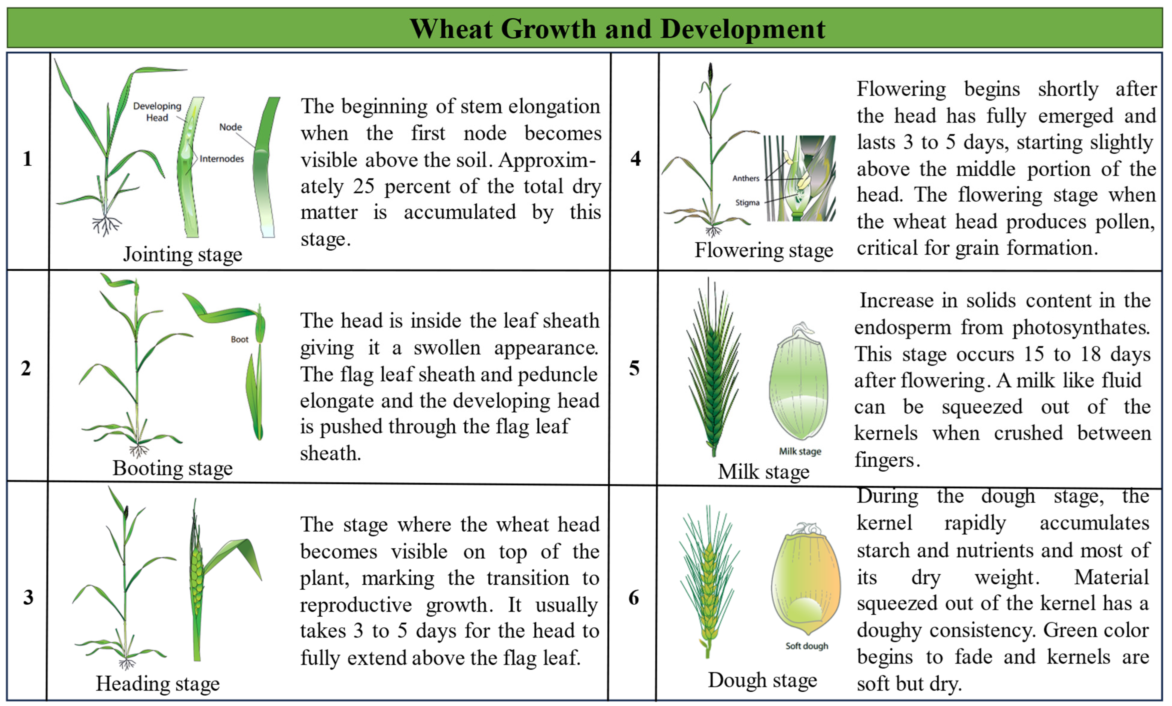
Multispectral data were collected using the DJI P4M UAV (SZ DJI Technology Co., Shenzhen, China) equipped with five multispectral sensors corresponding to Blue (450 ± 16 nm), Green (560 ± 16 nm), Red (650 ± 16 nm), Red-edge (730 ± 16 nm), and NIR (840 ± 26 nm). The data were collected between 10:00 a.m. and 2:00 p.m. under clear and windless conditions. The experiment lasted two years, and each flight could collect visible light and multispectral images simultaneously. The specific growth stages of wheat collected were as follows: jointing (19 March), booting (8 April), heading (14 April), flowering (18 April), milk (9 May), and dough (14 May) in 2023; the corresponding stages in 2024 were jointing (21 March), booting (30 March), heading (10 April), flowering (18 April), milk (8 May), and dough (16 May). To provide a more intuitive understanding of the characteristics of the key growth stages of winter wheat, Figure 2 presents visual illustrations for each growth stage along with corresponding textual descriptions.

Given the large study area and the limited battery life of the UAV, the mission was designed with 80% heading overlap and 75% side overlap at a flight speed of 5.2 m/s. The camera was set to capture images at 2 s intervals. Ten aerial survey points were established within the study area to ensure accurate geometric correction, and reflectance calibration was conducted using a gray gradient panel before each flight. The steps were as follows: First, UAV multispectral data were imported into Pix4D Mapper for image mosaic and geometric correction, using ground control points to generate a dense point cloud and a digital orthophoto. Then, the multispectral images were corrected for reflectance using the gray gradient calibration panel to produce accurate reflectance images. Finally, the regions of interest (ROIs) were defined for each sampling point in ENVI 5.3, and the average reflectance within each ROI was extracted to obtain the reflectance spectra of winter wheat at each sampling point.

2.2.2. Field Data

Field data collection for winter wheat was conducted simultaneously with UAV image acquisition to ensure consistent data gathering. Multiple sampling points were evenly distributed to ensure data accuracy based on the field’s area, as shown in Figure 1. Each sampling point covered an area of 1 m × 1 m, and the position of each point was recorded using a high-precision RTK device.

(1)

Chlorophyll Content Measurement

At each sampling point, 15 wheat plants with uniform growth were randomly selected. Chlorophyll content, expressed as SPAD values, was measured using a SPAD-502 Plus. The second-to-last leaf was measured for the jointing stage, while the fully expanded flag leaf was measured for the booting, heading, flowering, and grain-filling stages. Measurements were taken from the leaf’s upper, middle, and lower parts, avoiding the main stem veins, and the average value was calculated.

(2)

Leaf Area Index Measurement

The SunScan instrument measured the light transmission rate through the crop canopy, allowing for the leaf area index estimation. LAI data were collected from four randomly selected positions below the canopy in each sample, with eight readings taken. The average of these values was used as the LAI for the area. The instrument height was kept consistent during measurement, and the device automatically calculated LAI values.

(3)

Plant Height Measurement

A measuring tape was used to measure the distance from the soil surface to the top of the wheat plant’s leaves or spikes in their natural state, providing the plant height data. Fifteen uniformly growing wheat plants were randomly selected from each plot, and their average height was used as the wheat height for that plot.

(4)

Biomass Measurement

At each sampling point, 15 wheat plants were selected and separated into stems, leaves, and spikes. The samples were then initially dried in an oven at 105 °C for 30 min and then baked at 80 °C for at least 48 h until constant weight. The dry weight was recorded, and biomass was calculated by dividing this value by the sampling area.

(5)

Plant Water Content Measurement

Wheat stems, leaves, and spikes were separated, and both their fresh and dry weights were recorded. PWC was calculated using the following formula [14]:

$$\mathrm{P}\mathrm{W}\mathrm{C}={\displaystyle \frac{\left(\mathrm{p}\mathrm{l}\mathrm{a}\mathrm{n}\mathrm{t} \mathrm{f}\mathrm{r}\mathrm{e}\mathrm{s}\mathrm{h} \mathrm{w}\mathrm{e}\mathrm{i}\mathrm{g}\mathrm{h}\mathrm{t}-\mathrm{p}\mathrm{l}\mathrm{a}\mathrm{n}\mathrm{t} \mathrm{d}\mathrm{r}\mathrm{y} \mathrm{w}\mathrm{e}\mathrm{i}\mathrm{g}\mathrm{h}\mathrm{t}\right)}{\mathrm{p}\mathrm{l}\mathrm{a}\mathrm{n}\mathrm{t} \mathrm{f}\mathrm{r}\mathrm{e}\mathrm{s}\mathrm{h} \mathrm{w}\mathrm{e}\mathrm{i}\mathrm{g}\mathrm{h}\mathrm{t}}}\times 100\%.$$

(1)

(6)

Yield Measurement

After the wheat reached maturity, an area of 1 m² was randomly selected from each plot for harvest, and the number of spikes was recorded. The number of grains per spike and the thousand-kernel weight were measured in the laboratory, and yield data for each plot were calculated.

2.3. Research Methods

2.3.1. Selection of Vegetation Index

Differences in crop biochemical parameters can lead to variations in spectral reflectance characteristics [16,17,18]. The Vegetation Index (VI) is calculated through linear or nonlinear combinations of spectral bands to enhance vegetation features while minimizing interference from soil backgrounds and other factors. This approach allows for a more accurate reflection of vegetation growth status and health levels. Based on a review of the relevant literature, this study constructed 30 commonly used and representative VIs utilizing multispectral data collected from five spectral bands. The VIs and calculation formulas used in this paper are shown in

Table 1. Spectral vegetation indices used in this study.

Vegetation Index	Formula	References
Normalized difference vegetation index (NDVI)	$NDVI=(nir-r)/(nir+r)$	[19,20]
Transformed difference vegetation index (TDVI)	$TDVI=1.5\ast \left(nir-r\right)/\sqrt{{nir}^2+r+0.5}$	[19]
Green normalized difference vegetation index (GNDVI)	$GNDVI(=nir-g)/(nir+g)$	[20,21]
Normalized difference red-edge (NDRE)	$NDRE=(nir-re)/(nir+re)$	[20,22]
Renormalized difference vegetation index (RDVI)	$RDVI=(nir-r)/\left(\sqrt{nir+r}\right)$	[23,24]
Difference vegetation index (DVI)	$DVI=nir-r$	[23,25]
Visible atmospherically resistant index (VARI)	$VARI=(g-r)/(g+r-b)$	[26]
Ratio vegetation index (RVI)	$RVI=r/nir$	[23]
Simple ratio (SR)	$SR=nir/r$	[24,27]
Modified simple ratio (MSR)	$MSR=(nir/r-1)/\left(\sqrt{nir/r+1}\right)$	[24,28]
Enhanced vegetation index (EVI)	$EVI=2.5\ast (nir-r)/(nir+6r-7.5b+1)$	[23]
Enhanced vegetation index 2 (EVI2)	$EVI2=2.5\ast (nir-r)/(1+nir+2.4r)$	[23]
Soil adjusted vegetation index (SAVI)	$SAVI=1.5\ast (nir-r)/(nir+r+0.5)$	[29]
Optimized soil adjusted vegetation index (OSAVI)	$OSAVI=1.16\left(nir-r\right)/(nir+r+0.16)$	[28]
Green soil-adjusted vegetation index (GSAVI)	$GSAVI=1.5\ast (nir-g)/(nir+g+0.5)$	[30]
Green optimized soil-adjusted vegetation index (GOSAVI)	$GOSAVI=(nir-g)/(nir+g+0.16)$	[31]
Modified soil-adjusted vegetation index 2 (MSAVI2)	$MSAVI2=(2nir+1-\sqrt{{\left(2nir+1\right)}^2-8\ast \left(nir-r\right)})/2$	[32]
Green chlorophyll index (GCI)	$GCI=nir/g-1$	[20]
Red-edge chlorophyll index (RECI)	$RECI=nir/re-1$	[33]
Green-red vegetation index (GRVI)	$GRVI=(g-r)/(g+r)$	[34]
Green-blue vegetation index (GBVI)	$GBVI=(g-b)/(g+b)$	[34]
Simplified canopy chlorophyll content index (SCCCI)	$SCCCI=NDRE/NDVI$	[35]
Modified chlorophyll absorption in reflectance index (MCARI)	$MCARI=\left[\left(re-r\right)-0.2\ast \left(re-g\right)\right](re/r)$	[28,34]
Transformed chlorophyll absorption in reflectance index (TCARI)	$TCARI=3\left[\left(re-r\right)-0.2\ast \left(re-g\right)\right](re/r)$	[28,34]
MCARI/OSAVI	MCARI/OSAVI	[28]
TACRI/OSAVI	TACRI/OSAVI	[28]
Wide dynamic range vegetation index (WDRVI)	$WDRVI=(0.12\ast nir-r)/(0.12\ast nir+r)$	[36]
Non-linear index (NLI)	$NLI=({nir}^2-r)/({nir}^2+r)$	[24]
Modified non-linear index (MNLI)	$MNLI={1.5\ast (nir}^2-r)/({nir}^2+r+0.5)$	[24]
Triangular vegetation index (TVI)	$TVI=60\ast \left(nir-g\right)-100\ast \left(r-g\right)$	[37]

Note: $r$, $g$, $b$, $re$, and $nir$ correspond to the reflectivity of red, green, blue, red edge, and near-infrared bands, respectively.

.

2.3.2. Modeling Method

LR is one of the most commonly used methods for regression analysis, which assumes a linear relationship between independent and dependent variables during the modeling process. LR can effectively fit the data and derive regression coefficients by minimizing the sum of squared errors. However, it is limited to capturing linear relationships and performs poorly with complex nonlinear data [38]. On the other hand, RF uses an ensemble learning method, creating multiple decision trees by generating sub-datasets through bootstrapping. This approach is well-suited for capturing complex nonlinear relationships between variables and is highly resistant to overfitting [39]. GB is another method that trains multiple models in sequence, improving prediction by correcting the errors made by previous models. GB demonstrates predictive solid power, especially when modeling nonlinear data [40]. SVR is based on Support Vector Machines and aims to maximize the margin while finding the optimal regression function. It is particularly effective for high-dimensional data modeling and performs well with small sample sizes [41]. To provide a more intuitive understanding of the performance differences among the four models, Figure 3 shows radar charts of the four models in terms of model complexity, training time, data scale, interpretability, and noise robustness.

2.3.3. Comprehensive Growth Index (CGI)

(1)

CGI construction based on the equal-weight method

The construction of the comprehensive growth index (CGIav) using the equal-weight method assigns equal weights to various crop growth indicators to evaluate the overall growth status of the crops [14]. The process is as follows: First, growth parameters such as LAI, PH, and SPAD are normalized using the Min-Max Scaling method [42]. Then, the equal weight $w_i={\displaystyle \frac{1}{n}}$ is assigned to each standardized indicator, where n represents the number of selected growth indicators. Finally, the standardized values are multiplied by their respective weights and summed to obtain CGIav, as shown in the following formula:

$${\overline{X}}_i={\displaystyle \frac{X_i-\min \left(X_i\right)}{\max \left(X_i\right)-\min \left(X_i\right)}},$$

(2)

$${CGI}_{\mathrm{a}\mathrm{v}}=\sum _{i=1}^n{w}_i\times {\overline{X}}_i,$$

(3)

where ${\overline{X}}_i$ represents the normalized value of the i-th growth indicator and $\mathrm{m}\mathrm{a}\mathrm{x}\left(X_i\right)$ and ${\mathrm{m}\mathrm{i}\mathrm{n}(X}_i)$ are the maximum and minimum values in the i-th indicator, respectively. This study’s selected indicators include PH, LAI, BM, SPAD, and PWC.

(2)

CGI construction based on the coefficient of variation method

Xu et al. [15], recognizing the varying importance of different crop parameters in CGI, developed CGIcv using the coefficient of variation (CV) method, achieving significant results. Since then, this method has been widely applied in constructing CGI. The coefficient of variation method determines the weight of each evaluation index based on the degree of variation in the values of the indices, and the calculation is not affected by the scale of the data. The larger the coefficient of variation, the more informative the index, and the greater the weight assigned to it; conversely, a smaller coefficient of variation results in a smaller weight. The calculation formulas are as follows:

$$V_i={\displaystyle \frac{{\sigma }_i}{{\overline{x}}_i}},$$

(4)

$$W_i={\displaystyle \frac{V_i}{\sum _{i=1}^n{V}_i}},$$

(5)

where $V_i$ is the coefficient of variation for the i-th index, ${\sigma }_i$ is the standard deviation of the i-th index, ${\overline{x}}_i$ is the mean value of the i-th index, and $W_i$ is the weight assigned to the i-th index.

Based on field-measured data and the coefficient of variation method, the CGIcv for winter wheat was constructed. The specific approach was as follows: First, the weights for the five indices (PH, LAI, BM, SPAD, and PWC) were calculated using Equations (4) and (5); then, each index was normalized according to Equation (2). Finally, the weighted sum of all standardized indices yielded CGIcv, as described by the formula:

$${CGI}_{CV}=\sum _{i=1}^5{W}_i{\overline{X}}_i.$$

(6)

(3)

CGI construction based on the contribution of single indicators to yield

Accurately capturing crop growth information in modern agriculture is vital for yield forecasting and effective management. Remote sensing-based crop growth monitoring typically depends on single indicators such as the LAI, PH, or BM. However, these single metrics do not provide a complete picture of crop growth. Crop growth is influenced by numerous physiological and structural parameters, with different contributions to yield depending on the growth stage. Therefore, integrating multiple indicators and fully accounting for their yield contributions is essential for improving monitoring precision. An adaptive weight allocation method based on the yield contributions of growth indicators is proposed to capture crop growth information and predict yield. This approach provides a comprehensive and dynamic evaluation of crop growth and optimizes its application in crop growth monitoring.

(1)

Principle of Construction

The core principle of the method is to construct CGIac by dynamically assigning weights to various growth indicators (e.g., PH, LAI, BM, SPAD, and PWC) at different growth stages based on their contribution to yield. Specifically, crop yields are affected not just by a single parameter at a given growth stage, but by a combination of several parameters throughout the growth cycle. The model uses data from multiple growth stages and several growth parameters, and regression analysis is employed to determine the contribution of each parameter at different stages to yield formation. Based on these contributions, the CGIac is constructed.

(2)

Data Pre-processing and Feature Matrix Construction

Before constructing CGIac, key structural and physiological parameters at different growth stages must be collected. For example, data for winter wheat at the jointing, booting, heading, flowering, milk, and dough stages include PH, LAI, BM, SPAD, and PWC. These data are organized into a matrix form, resulting in the growth feature matrix X:

$$X=\left[\begin{array}{cccc}{x}_{11}& x_{12}& \cdots & x_{1j}\\ x_{21}& x_{22}& \cdots & x_{2j}\\ ⋮& ⋮& \ddots & ⋮\\ x_{i1}& x_{i2}& \cdots & x_{ij}\end{array}\right],$$

(7)

where $x_{ij}$ represents the value of the j-th growth parameter at the i-th growth stage. This matrix contains data from i growth stages and j different parameters.

(3)

Calculation of the weight matrix

To appropriately allocate the weights of each growth parameter, it is necessary to adaptively assign weights based on each parameter’s contribution to yield. First, the mapping relationship between the growth parameters and yield for each growth stage is calculated using linear regression (LR) or nonlinear regression models (RF, GB, SVR). For each growth parameter $x_{ij}$ at a specific growth stage, its contribution to yield Y can be estimated using the following regression model:

$$Y=f\left(x_{11},x_{12},\cdots ,x_{ij}\right).$$

(8)

The contribution rate of each parameter can be obtained through training and validation of the model. These contribution rates are then represented as a weight matrix $W$ for the different parameters at each growth stage.

(4)

Calculation of the CGIac

To eliminate the effect of magnitude between different parameters, it is first necessary to normalize each parameter. In this study, the Min-Max Scaling method was applied for normalization, as shown in Equation (2). Using the weight matrix $W$ and the normalized growth feature matrix $X$, the comprehensive growth monitoring index CGIac can be calculated. This process is achieved through matrix multiplication:

$$\begin{gathered} CG{I}_{ac}=X\cdot W^{\mathrm{T}}=\left[G_1,G_2,\dots ,G_m\right]= \\ \left[\begin{array}{cccc}{x}_{11}& x_{12}& \cdots & x_{1j}\\ x_{21}& x_{22}& \cdots & x_{2j}\\ ⋮& ⋮& \ddots & ⋮\\ x_{i1}& x_{i2}& \cdots & x_{ij}\end{array}\right]\cdot {\left[\begin{array}{cccc}{w}_{11}& w_{12}& \cdots & w_{1j}\\ w_{21}& w_{22}& \cdots & w_{2j}\\ ⋮& ⋮& \ddots & ⋮\\ w_{i1}& w_{i2}& \cdots & w_{ij}\end{array}\right]}^{\mathrm{T}}. \end{gathered}$$

(9)

The matrix multiplication calculates the comprehensive index for each growth stage based on the contributions of different growth parameters. The result is a comprehensive growth index vector $G_1,G_2,\dots ,G_m$, where each $G_i$ represents the comprehensive growth monitoring index for the i-th growth stage. This index reflects the overall crop growth performance at each stage. Considering the contribution of different parameters to yield allows for a more accurate assessment of crop growth.

2.3.4. Evaluation Metrics

In this study, data from 2023 were used as the training set, while data from 2024 served as the test set to ensure the accuracy and reliability of model training and evaluation. After training, the model’s predictions were compared with the actual values from the test set to evaluate performance and prediction accuracy. The model was assessed on the validation set using the Coefficient of Determination (R²) and Root Mean Square Error (RMSE). The closer the R² value is to 1, the stronger the model can explain the target variable, indicating a higher consistency between predicted and actual values. A smaller RMSE value reflects a minor deviation between predicted and actual values, indicating a lower model error and higher prediction accuracy [14,15,43].

3. Results

3.1. Construction of CGIac

In this study, CGIac was constructed based on the varying contribution of individual growth parameters to yield across different growth stages.

Table 2. Construction of CGIac at different growth stages across multiple models.

Model	Growth Stage	CGIac
LR	Jointing	G1 = 0.271758 × BM + 0.304704 × LAI + 0.104303 × PH + 0.02197 × SPAD + 0.297265 × PWC
	Booting	G2 = 0.034661 × BM + 0.433267 × LAI + 0.006892 × PH + 0.253023 × SPAD + 0.272156 × PWC
	Heading	G3 = 0.011324 × BM + 0.489689 × LAI + 0.236703 × PH + 0.099299 × SPAD + 0.162987 × PWC
	Flowering	G4 = −0.0766 × BM + 0.277624 × LAI + 0.440874 × PH + 0.066658 × SPAD + 0.138243 × PWC
	Milk	G5 = −0.30049 × BM + 0.324447 × LAI + 0.250528 × PH − 0.06709 × SPAD − 0.05745 × PWC
	Dough	G6 = −0.18787 × BM + 0.441084 × LAI + 0.135365 × PH + 0.00168 × SPAD − 0.234 × PWC
RF	Jointing	G1 = 0.17298 × BM + 0.341312 × LAI + 0.259386 × PH + 0.123208 × SPAD + 0.103113 × PWC
	Booting	G2 = 0.014361 × BM + 0.829011 × LAI + 0.018984 × PH + 0.046781 × SPAD + 0.090864 × PWC
	Heading	G3 = 0.041499 × BM + 0.602172 × LAI + 0.209805 × PH + 0.062957 × SPAD + 0.083567 × PWC
	Flowering	G4 = 0.058259 × BM + 0.088018 × LAI + 0.747809 × PH + 0.052486 × SPAD + 0.053429 × PWC
	Milk	G5 = 0.080248 × BM + 0.406717 × LAI + 0.188087 × PH + 0.098313 × SPAD + 0.226635 × PWC
	Dough	G6 = 0.065111 × BM + 0.721612 × LAI + 0.080778 × PH + 0.049925 × SPAD + 0.082573 × PWC
GB	Jointing	G1 = 0.213924 × BM + 0.354581 × LAI + 0.171247 × PH + 0.164739 × SPAD + 0.095509 × PWC
	Booting	G2 = 0.010774 × BM + 0.816524 × LAI + 0.020577 × PH + 0.045704 × SPAD + 0.106421 × PWC
	Heading	G3 = 0.032358 × BM + 0.722393 × LAI + 0.099169 × PH + 0.084201 × SPAD + 0.061879 × PWC
	Flowering	G4 = 0.057654 × BM + 0.097934 × LAI + 0.739065 × PH + 0.06869 × SPAD + 0.036656 × PWC
	Milk	G5 = 0.07444 × BM + 0.461609 × LAI + 0.139829 × PH + 0.102316 × SPAD + 0.221806 × PWC
	Dough	G6 = 0.079261 × BM + 0.702568 × LAI + 0.079209 × PH + 0.036209 × SPAD + 0.102752 × PWC
SVR	Jointing	G1 = 0.29722 × BM + 0.21063 × LAI + 0.113377 × PH + 0.070007 × SPAD + 0.308767 × PWC
	Booting	G2 = 0.126434 × BM + 0.285509 × LAI + 0.212022 × PH + 0.164219 × SPAD + 0.211816 × PWC
	Heading	G3 = 0.153201 × BM + 0.357273 × LAI + 0.206744 × PH + 0.092045 × SPAD + 0.190736 × PWC
	Flowering	G4 = 0.13485 × BM + 0.222092 × LAI + 0.406385 × PH + 0.107272 × SPAD + 0.129401 × PWC
	Milk	G5 = 0.292152 × BM + 0.230943 × LAI + 0.273961 × PH + 0.078397 × SPAD + 0.124547 × PWC
	Dough	G6 = 0.415469 × BM + 0.322669 × LAI + 0.120148 × PH + 0.072594 × SPAD + 0.069119 × PWC

presents the CGIac developed for different growth stages using the LR, RF, GB, and SVR models. There were notable differences in the weight distribution of SPAD, LAI, PH, BM, and PWC across these stages and models.

During the booting and heading stages, LAI contributed significantly to yield. In the RF model, the weight of LAI during the booting stage was 0.829011, while in the GB model, it was 0.722393. At the heading stage, LAI’s weight was 0.602172 in the RF model and 0.722393 in the GB model. However, LAI’s weight decreased as the growth progressed to the flowering stage. For example, in the LR model, LAI’s weight dropped from 0.489689 at the heading stage to 0.277624 at the flowering stage. In summary, LAI had the highest contribution during the booting and heading stages, particularly in the RF and GB models.

SPAD weights also varied across the models. At the jointing stage, SPAD’s weight was 0.02197 in the LR model but 0.123208 in the RF model. At the booting stage, SPAD’s weight was 0.253023 in the LR model and 0.046781 in the RF model, while at the heading stage, SPAD’s weight was 0.099299 in the LR model and 0.062957 in the RF model. These results suggest that SPAD plays a more important role during earlier growth stages, with the LR model being particularly sensitive to SPAD variations.

The contribution of PH and BM to yield also varied across the growth stages. At the flowering stage, PH reached its highest weight (0.440874) in the LR model. However, its weight decreased during the milk stage and dropped to 0.135365 at the dough stage. Conversely, BM’s weight increased during the later growth stages, especially in the SVR model, where BM’s weight at the dough stage was 0.415469, compared to just 0.126434 at the flowering stage. This suggests that while PH is critical during earlier stages, BM becomes more influential as the crop matures, particularly in the SVR model.

PWC’s weight fluctuated across models and growth stages. During the booting stage, PWC’s weight was 0.272156 in the LR model and 0.211816 in the SVR model. However, at the dough stage, PWC’s weight was relatively low across most models, reaching just 0.069119 in the SVR model and even turning negative in the LR model (−0.234). PWC showed variable importance depending on the stage, with its influence diminishing by the dough stage.

In summary, the weight allocation of growth parameters varied significantly across growth stages and models. The RF and GB models gave higher weights to LAI during the booting and heading stages, while the SVR model assigned more weight to BM during the dough stage. In contrast, the LR model was more responsive to SPAD and PH during the earlier growth stages.

3.2. Performance Analysis of CGIac in Crop Yield

3.2.1. Correlation Analysis Between CGIac and Yield

To analyze the relationship between the CGIac and wheat yield, Pearson correlation analysis was conducted for both individual growth indicators (BM, LAI, PH, SPAD, PWC) and CGIac with yield data. Figure 4 shows the correlations between CGIac and yield for different models in 2023 (a, b, c, and d) and 2024 (e, f, g, and h). The analysis below uses the 2023 data as an example.

In the correlation analysis of individual growth indicators, LAI, PH, and PWC exhibited higher correlations with yield during several growth stages. For instance, the LR model’s correlation coefficients for LAI, PH, and PWC during the heading stage were 0.88, 0.80, and 0.75, respectively. Conversely, BM and SPAD showed weaker correlations in most growth stages, particularly during the heading stage, where the correlation coefficient for BM was −0.60 and for SPAD was just 0.2. Compared to individual growth indicators, CGIac demonstrated a substantial improvement in yield correlation across all models. For example, in the LR model, the correlation for CGIac during the flowering stage was 0.92, a 24.32% increase over LAI’s 0.74. During the heading stage, the correlation for CGIac reached 0.94, a 6.8% increase from LAI’s 0.88. The correlation between CGIac and yield also showed notable improvements in other models. CGIac’s correlation during the flowering stage in the RF model was 0.86, a 16.2% increase over LAI’s 0.74. In the GB model, CGIac’s correlation increased from 0.74 (LAI) to 0.87 during the flowering stage, a 17.56% improvement.

Among the models, the LR model performed best in capturing the relationship between CGIac and yield, particularly during the flowering stage, where the correlation reached 0.92, significantly higher than LAI’s 0.74. This demonstrates the LR model’s ability to effectively capture the combined effects of multiple growth indicators on yield. The RF and GB models also performed well across various growth stages. For instance, in the GB model, the correlation for CGIac during the heading stage was 0.91. In contrast, the RF model reached 0.93, showing that these models can effectively handle complex multi-dimensional data and use growth indicators for accurate yield prediction. However, the SVR model performed better in earlier stages but experienced a decline in later stages. For example, in the heading stage, the correlation for CGIac in the SVR model was 0.93, but it decreased to 0.51 and 0.44 during the milk and dough stages, respectively.

To visually demonstrate the sensitivity distribution of CGIac constructed through different machine learning models and individual growth indicators on yield, Figure 5 presents a violin plot showing the sensitivity analysis of the correlation between different CGIac and individual indicators on yield. The results indicate that CGIac consistently exhibits a compact and stable high correlation across all models and years, with correlation coefficients concentrated between 0.8 and 1.0, showing minimal fluctuation. Taking the 2023 RF model as an example, the correlation of CGIac is close to 1.0, suggesting that this comprehensive index effectively integrates information from individual growth indicators to more accurately predict crop yield. This consistently high correlation proves the validity of CGIac’s adaptive weighting mechanism, where the allocation of weights to each growth indicator is reasonable, allowing the comprehensive index to stably reflect crop growth across different years and models.

LAI and PH are the individual indicators most closely correlated with yield, with correlation coefficients generally ranging between 0.5 and 0.7. However, their sensitivity shows significant variation. The violin plots reveal a wide range of distribution for these indicators across different years and models, with large extremes. For example, the correlation range of PH in the 2023 SVR model varies from 0.4 to 0.8, indicating high median values but substantial changes depending on the environment and model. The correlation of LAI in the 2024 RF model fluctuates even more, with coefficients ranging from 0.3 to 0.7, indicating that its influence on yield is unstable. PWC (Plant Water Content) shows large fluctuations in sensitivity across different years and models. In the 2023 RF model, PWC’s correlation coefficients are concentrated between 0.4 and 0.8, indicating that water conditions significantly impacted yield that year. However, in the 2024 LR model, PWC’s correlation weakens, with coefficients fluctuating between 0.0 and 0.5, showing a decline in its relevance. SPAD and BM performed less consistently compared to other indicators. The violin plots show that their correlation distributions are more scattered, with generally lower correlation coefficients.

The sensitivity analysis of individual growth indicators (LAI, SPAD, PH, BM, and PWC) deepens the understanding of CGIac’s adaptive weighting process. The results from the violin plots show that CGIac demonstrates high stability and correlation across all models and years, while the performance of individual indicators varies depending on the year, model, and environmental conditions. Therefore, reasonably adjusting the weights of each indicator ensures that CGIac maintains its efficiency and reliability in yield prediction across different growth stages and environmental conditions. This process not only optimizes model performance under varying conditions but also provides valuable guidance for field management, helping to address the challenges of complex and changing agricultural environments.

3.2.2. Comparative Analysis of the Correlation Between Different CGI and Crop Yield

To further investigate the correlation between various CGI and crop yield, we compared the indices constructed using the equal weight method (CGIav), the coefficient of variation method (CGIcv), and the yield contribution rate method (CGIac). Since the RF model’s weight distribution for parameters (such as LAI, PH, and SPAD) aligns well with real-world crop management practices, it demonstrates excellent generalization, effectively handling noise and outliers in the data. Thus, we selected the CGIac constructed with the RF model for this analysis. Pearson correlation coefficients were used to evaluate the relationship between individual growth indicators (BM, LAI, PH, SPAD, PWC), the three comprehensive indices, and yield. Figure 6 displays the correlation heatmaps across different years and methods.

The experimental results show that in both 2023 and 2024, LAI had the highest correlation with yield among the individual indicators, peaking during the heading stage with values of 0.88 in 2023 and 0.79 in 2024. LAI consistently demonstrated a strong positive correlation with yield across multiple growth stages in both years, indicating its significant influence on yield. In contrast, BM (biomass) and SPAD (relative chlorophyll content) showed relatively weak correlations. For example, BM’s correlation during the heading stage 2023 was −0.60, while SPAD’s was only 0.2. This may be due to the limited role of BM and SPAD in the later stages of crop growth, particularly as biomass accumulation does not directly represent the yield formation process.

Compared to individual growth indicators, CGIac showed a significant improvement in correlation with yield across different growth stages and years. For example, in 2023, CGIac achieved a correlation of 0.86 during the flowering stage, a 16.2% increase compared to LAI’s 0.74. In 2024, CGIac’s correlation during the flowering stage was 0.84, which was 21.7% higher than LAI’s 0.69. CGIav and CGIcv also improved their correlations with yield, but to a lesser extent. In 2023, CGIav’s correlation during the flowering stage was 0.83, an improvement of 12.16% over LAI’s 0.74. CGIcv had a correlation of 0.80 during the flowering stage, an 8.1% increase compared to LAI’s 0.74. However, CGIcv outperformed CGIav during the booting, heading, and dough stages, though it slightly underperformed CGIav during the flowering and milk stages. Further analysis revealed that CGIcv generally outperformed CGIav.

In conclusion, CGIac consistently displayed higher correlations across growth stages, models, and years, confirming its effectiveness for crop growth monitoring. These results demonstrate the superiority of using an adaptive weight allocation method based on yield contribution for crop monitoring, as it better captures the dynamic relationship between growth indicators and yield compared to equal-weight and coefficient of variation methods.

3.2.3. Evaluation of the Accuracy Variations in Yield Prediction with CGIac

To further evaluate the effectiveness of CGIac in yield prediction, we integrated CGIac, CGIav, and CGIcv into the prediction models and examined the changes in accuracy.

Table 3. Comparison of yield prediction accuracy of winter wheat with different CGI at each growth stage.

Growth Stages	Model	Without CGI		CGIac		CGIav		CGIcv
		R2	RMSE (t/ha)	R2	RMSE (t/ha)	R2	RMSE (t/ha)	R2	RMSE (t/ha)
Jointing	LR	0.370	0.0593	0.377	0.0587	0.370	0.0593	0.375	0.0589
	RF	0.379	0.0586	0.433	0.0535	0.337	0.0625	0.448	0.052
	GB	0.460	0.0508	0.478	0.0492	0.360	0.0603	0.478	0.0492
	SVR	0.366	0.0597	0.360	0.0603	0.366	0.0597	0.368	0.0595
Booting	LR	0.643	0.0336	0.643	0.0336	0.643	0.0336	0.644	0.0336
	RF	0.613	0.0365	0.622	0.0356	0.603	0.0374	0.605	0.0372
	GB	0.604	0.0373	0.623	0.0355	0.626	0.0352	0.619	0.0359
	SVR	0.499	0.0472	0.527	0.0446	0.497	0.0474	0.503	0.0468
Heading	LR	0.573	0.0402	0.573	0.0402	0.573	0.0402	0.575	0.0400
	RF	0.523	0.0450	0.541	0.0433	0.477	0.0493	0.474	0.0495
	GB	0.522	0.0451	0.530	0.0443	0.499	0.0472	0.532	0.0441
	SVR	0.380	0.0584	0.396	0.0569	0.376	0.0588	0.376	0.0588
Flowering	LR	0.757	0.0229	0.757	0.0229	0.757	0.0229	0.755	0.0231
	RF	0.756	0.0230	0.780	0.0207	0.762	0.0224	0.757	0.0229
	GB	0.755	0.0231	0.772	0.0215	0.768	0.0219	0.736	0.0249
	SVR	0.571	0.0404	0.586	0.0390	0.573	0.0402	0.607	0.037
Milk	LR	0.380	0.0584	0.468	0.0501	0.341	0.0621	0.268	0.069
	RF	0.588	0.0389	0.637	0.0342	0.560	0.0415	0.426	0.0541
	GB	0.584	0.0392	0.551	0.0423	0.602	0.0375	0.239	0.0717
	SVR	0.363	0.0600	0.411	0.0555	0.384	0.0580	0.235	0.0721
Dough	LR	0.544	0.0429	0.544	0.0429	0.544	0.0429	0.546	0.0428
	RF	0.600	0.0377	0.589	0.0387	0.594	0.0382	0.575	0.0400
	GB	0.574	0.0402	0.545	0.0429	0.557	0.0417	0.507	0.0464
	SVR	0.362	0.0601	0.381	0.0584	0.375	0.0589	0.374	0.0590

Note: Bold values indicate improvements over the baseline model.

presents the results, with bolded values indicating improvements over the baseline model (without CGI). Across all models, the addition of CGI features enhanced prediction accuracy, although the magnitude of improvement varied. CGIac produced the largest accuracy gain, with a maximum improvement of 23.14%. CGIcv achieved up to 18.34% improvement, while CGIav led to a maximum increase of 5.7%. Among the models, CGIac showed the most significant impact, especially in the RF and GB models, where it excelled during the milk and jointing stages. For example, in the RF model, the R² increased from 0.588 to 0.637 during the milk stage after adding CGIac, with the RMSE decreasing from 0.0389 to 0.0342. Similarly, the GB model achieved an R² of 0.602 and an RMSE of 0.0375 after adding CGIcv during the milk stage, demonstrating strong performance.

The CGIac demonstrated strong robustness in capturing crop growth information, particularly in the RF and GB models. In contrast, CGIav and CGIcv provided less improvement, especially in the LR and SVR models. Overall, CGIac outperformed other features across multiple growth stages and models, offering reliable support for crop yield prediction.

In practical applications, CGIav stands out for its simplicity. By assigning equal weights to all growth indicators, CGIav has the lowest computational complexity, requiring minimal resources, making it a cost-effective option for small farms with limited computing capacity. However, this simplicity comes at the cost of prediction accuracy, especially in environments where crop growth and yield exhibit significant variability. This limits its effectiveness for precision agriculture management.

CGIcv, on the other hand, applies statistical analysis to the variability of growth indicators, assigning weights accordingly. While its computational complexity is slightly higher than that of CGIav, it remains manageable. CGIcv’s advantage lies in its adaptability to different growth stages and indicator variability, making it suitable for situations with high data variability, such as diverse growth conditions across fields. Therefore, CGIcv is more appropriate for medium-sized farms, providing more accurate field operation guidance.

CGIac uses the yield contribution rate method to dynamically allocate weights through regression models, resulting in the highest computational complexity. It not only analyzes the relationships between multiple growth indicators and yield but also handles complex nonlinear relationships. Due to its higher computational requirements, it may need more powerful computing resources. However, this method provides greater prediction accuracy, making it the ideal comprehensive growth index for large-scale precision agriculture management. Despite its higher computational complexity, CGIac can significantly optimize resource allocation and increase yield for large farms that prioritize high-precision predictions and data-driven decision making.

3.3. Construction of CGI Inversion Model

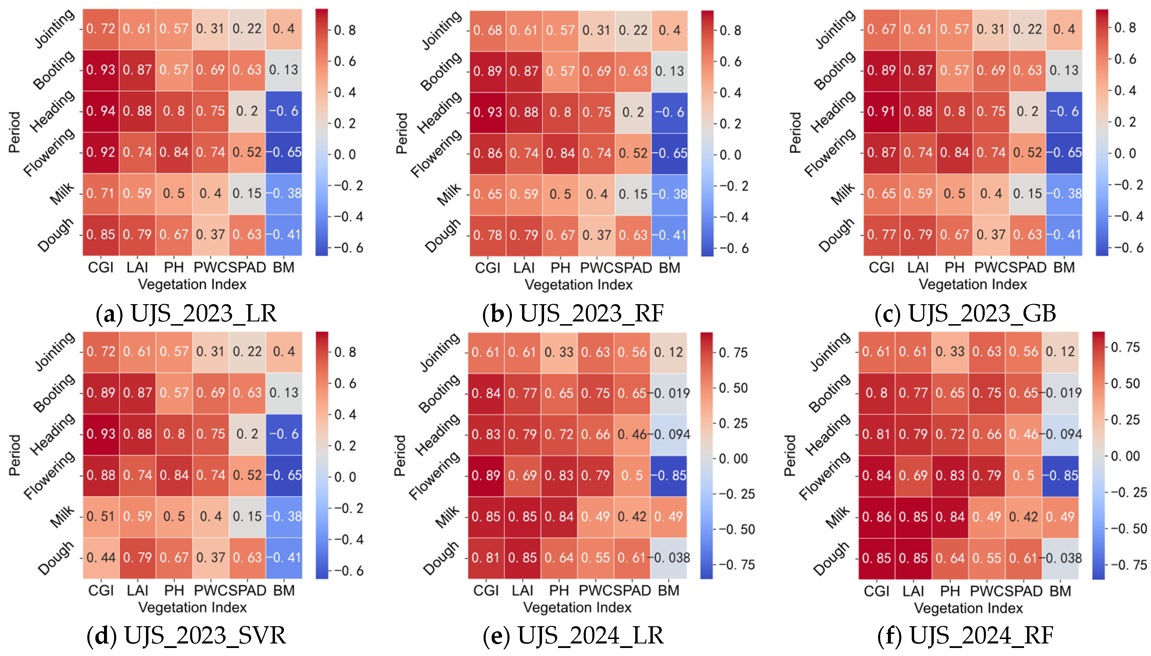
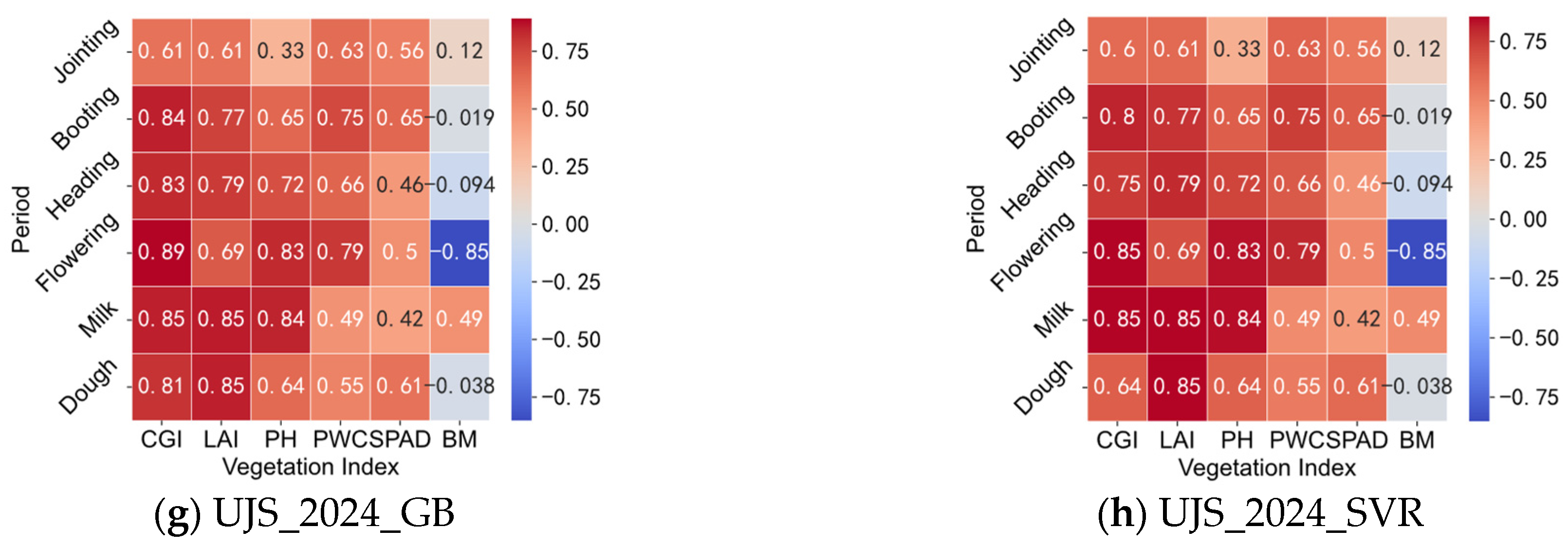
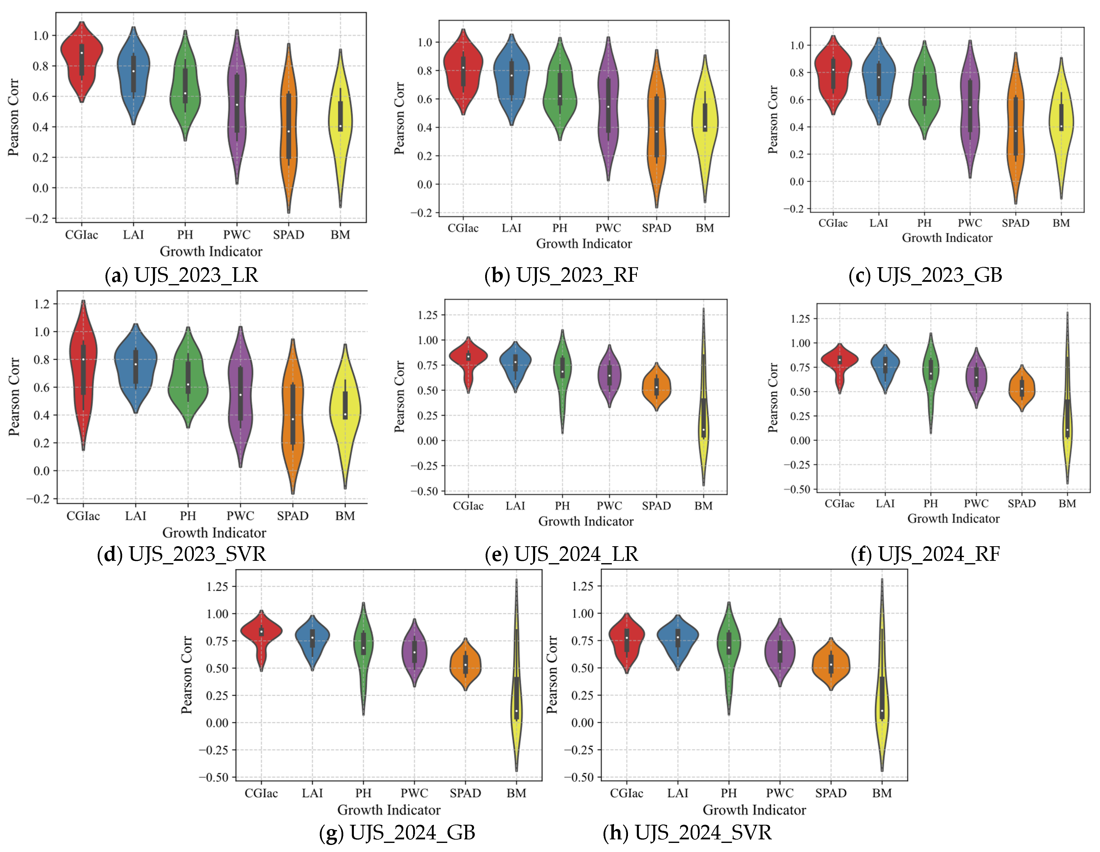
3.3.1. Correlation Analysis Between Vegetation Indices and CGIac

To analyze the relationship between the CGIac and the selected VIs, we used data from 2023 as a case study. First, we conducted a Pearson correlation analysis between CGIac and 30 commonly used VIs, followed by a significance test using p-values.

Table 4. The absolute values of correlation coefficients between vegetation index and CGI at different growth stages.

VI	Jointing	Booting	Heading	Flowering	Milk	Dough
RECI	0.775 **	0.748 **	0.760 **	0.906 **	0.815 **	0.923 **
NDRE	0.761 **	0.743 **	0.757 **	0.908 **	0.828 **	0.919 **
SCCCI	0.739 **	0.736 **	0.753 **	0.873 **	0.826 **	0.904 **
GOSAVI	0.753 **	0.896 **	0.892 **	0.894 **	0.780 **	0.890 **
GCI	0.743 **	0.701 **	0.710 **	0.916 **	0.789 **	0.919 **
GSAVI	0.771 **	0.911 **	0.910 **	0.864 **	0.752 **	0.860 **
OSAVI	0.762 **	0.883 **	0.887 **	0.861 **	0.718 **	0.852 **
GNDVI	0.716 **	0.676 **	0.686 **	0.910 **	0.806 **	0.905 **
MSAVI2	0.774 **	0.904 **	0.906 **	0.845 **	0.707 **	0.822 **
RDVI	0.772 **	0.899 **	0.902 **	0.848 **	0.712 **	0.837 **
EVI	0.776 **	0.903 **	0.908 **	0.837 **	0.711 **	0.841 **
MNLI	0.781 **	0.90 **	0.905 **	0.844 **	0.710 **	0.841 **
SAVI	0.767 **	0.900 **	0.904 **	0.841 **	0.706 **	0.824 **
SR	0.734 **	0.690 **	0.689 **	0.889 **	0.718 **	0.897 **
EVI2	0.771 **	0.903 **	0.905 **	0.840 **	0.705 **	0.821 **
NLI	0.716 **	0.786 **	0.806 **	0.873 **	0.719 **	0.865 **
MSR	0.725 **	0.675 **	0.674 **	0.887 **	0.722 **	0.896 **
TDVI	0.767 **	0.903 **	0.907 **	0.831 **	0.697 **	0.797 **
DVI	0.771 **	0.907 **	0.907 **	0.824 **	0.688 **	0.768 **
WDRVI	0.703 **	0.648 **	0.651 **	0.880 **	0.722 **	0.895 **
TVI	0.749 **	0.902 **	0.904 **	0.815 **	0.668 **	0.747 **
NDVI	0.684 **	0.628 **	0.630 **	0.872 **	0.714 **	0.867 **
VARI	0.612 **	0.602 **	0.585 **	0.765 **	0.396 *	0.766 **
MCARI	0.512 **	0.725 **	0.738 **	0.664 **	0.453 **	0.662 **
GRVI	0.468 **	0.460 **	0.360 *	0.679 **	0.302	0.719 **
MCAR/IOSAVI	0.381 *	0.628 **	0.643 **	0.565 **	0.253	0.313
TCARI/OSAVI	0.568 **	0.621 **	0.613 **	0.759 **	0.685 **	0.893 **
TCARI	0.568 **	0.682 **	0.671 **	0.777 **	0.685 **	0.918 **
GBVI	0.550 **	0.682 **	0.775 **	0.734 **	0.740 **	0.805 **
RVI	0.679 **	0.624 **	0.626 **	0.871 **	0.711 **	0.852 **

Note: * indicates significant at the 0.05 level, ** indicates significant at the 0.01 level.

represents the correlation between each VI and CGIac at different growth stages. The results showed that most VIs exhibited significant correlations with CGIac, passing the significance test, except for GRVI during the milk stage and MCAR and IOSAVI during the milk and dough stages.

The experimental results demonstrate that many VIs strongly correlated with CGIac at different growth stages, particularly RECI, NDRE, SCCCI, and GOSAVI, all with correlations exceeding 0.7 from the jointing stage to the dough stage. RECI consistently showed a correlation higher than 0.75 across all growth stages, peaking during the dough stage (r = 0.923). NDRE had its highest correlation during the flowering stage (r = 0.908), while GOSAVI showed very high correlations during the booting stage (r = 0.896), heading stage (r = 0.892), and flowering stage (r = 0.894). GSAVI and OSAVI also demonstrated significant correlations during the booting and heading stages. For example, GSAVI had correlations of 0.911 at the booting stage and 0.910 at the heading stage, while OSAVI showed correlations of 0.883 and 0.887 during these stages, respectively. These findings suggest that these indices can accurately reflect crop growth conditions during the early reproductive stages and have high applicability for growth monitoring.

Conversely, GRVI and MCAR/IOSAVI exhibited weaker correlations during all growth stages, particularly during the milk and dough stages, where they did not pass the significance test. For instance, GRVI correlated 0.360 during the heading stage and only 0.302 during the milk stage. Similarly, VARI had a low correlation during the milk stage, with a value of just 0.396, indicating its limited ability to monitor crop growth during this period.

Generally, the flowering stage exhibited the strongest correlations between multiple VIs and CGIac, with several indices achieving correlations above 0.8. For instance, NDRE (r = 0.908), GCI (r = 0.916), and GNDVI (r = 0.910) all showed very high correlations during this stage. Although some indices, such as RECI, NDRE, and SCCCI, maintained high correlations during the milk stage, others, like VARI, MCARI, and GRVI, showed a significant drop in correlation, with some failing the significance test.

3.3.2. Selection of Input Features

VIs are typically generated through linear or nonlinear calculations of multiple single bands and often exhibit strong multicollinearity, leading to instability in regression models [44]. Feature selection can effectively remove redundant information, reduce model complexity, and improve the stability and accuracy of prediction results. Elastic Net, an embedded feature selection method, combines the strengths of Ridge Regression and Lasso Regression, making it particularly suitable for linear regression problems where features are highly correlated or where the number of features exceeds the number of samples [45]. By applying L1 and L2 regularization to the regression coefficients, Elastic Net overcomes Lasso’s tendency to over-select variables in certain situations while addressing Ridge’s limitations in eliminating irrelevant variables. The regularization expression for Elastic Net is as follows:

$$L\left(\beta \right)=\underset{\beta }{\min }{\displaystyle \frac{1}{2n}}{‖X_i^T\beta -y_i‖}_2^2+\lambda \left[\alpha {‖\beta ‖}_1+(1-\alpha ){‖\beta ‖}_2^2\right],$$

(10)

where $X_i$ is the feature vector of the i-th sample, $y_i$ is the target value (CGIac) of the i-th sample, $\beta$ is the coefficient for the feature weights, $\lambda$ is the regularization strength parameter controlling the degree of regularization with a range of $\lambda \in (0,+\infty )$, and $\alpha$ is the weight between L1 regularization (Lasso) and L2 regularization (Ridge), with a range of $\alpha \in \left[0,1\right]$. When $\alpha =1$, Elastic Net reduces to Lasso Regression; when $\alpha =0$, it reduces to Ridge Regression. The model helps in selecting relevant features while reducing redundancy. In this experiment, we set α to [0.1, 0.2, 0.3, 0.5, 0.7, 0.9, 0.95, 1]. The parameter λ controls the strength of regularization, where larger values correspond to stronger regularization. We use “np.logspace(−4, 0, 50)” to generate 50 values for λ, logarithmically spaced between 10⁻⁴ (0.0001) and 10⁰ (1). The optimal values of the parameters α and λ for each growth period are summarized in

Table 5. The optimal values of elastic network parameters α and λ at each growth stage.

Growth Stages	λ (log10)	α
Jointing	−4	0.95
Booting	−3.428	1.0
Heading	−3.674	1.0
Flowering	−3.837	0.9
Milk	−2.937	1.0
Dough	−1.798	0.1

.

The model helps in selecting relevant features while reducing redundancy.

Table 6. Results of feature weight coefficients based on the elastic network model.

VI	Jointing	Booting	Heading	Flowering	Milk	Dough
DVI	0.2513	0.0000	0.0000	0.1197	0.0191	0.0000
EVI2	0.0000	0.0000	0.0000	0.0000	0.0137	0.0000
EVI	0.0000	0.0000	0.0000	0.0000	0.0160	0.0000
GBVI	−0.1370	0.0000	0.1892	0.1895	−0.0705	−0.0866
GCI	−0.3909	0.0000	−0.1293	0.0212	0.0284	0.0751
GNDVI	0.1826	0.0000	−0.8979	0.0582	0.0500	0.0609
GOSAVI	0.0057	0.0000	0.0000	0.0000	0.0333	0.0255
GRVI	0.1198	0.0000	0.0608	−0.1715	0.0000	0.0000
GSAVI	0.0567	0.0000	0.0000	0.0000	0.0293	0.0000
MCARI/OSAVI	−0.0058	0.0000	0.0000	0.0000	0.0000	0.0000
MCARI	−0.0173	0.0000	0.0000	0.0000	0.0000	0.0000
MNLI	0.5396	1.0156	0.0000	0.2467	0.0233	0.0000
MSAVI2	0.0000	0.0000	1.0549	0.0434	0.0148	0.0000
MSR	0.2019	0.0000	0.0000	0.0000	0.0006	0.0469
NDRE	0.0000	0.0000	0.0000	0.1745	0.0814	0.0585
NDVI	0.0000	0.0000	0.0000	0.0000	0.0000	0.0223
NLI	−0.3420	0.0000	0.0000	−0.1883	0.0000	0.0137
OSAVI	−0.3324	0.0000	0.0000	0.0000	0.0027	0.0000
RDVI	0.0000	0.0000	0.0000	0.0000	0.0096	0.0000
RECI	0.1256	0.0000	0.0000	0.1635	0.0597	0.0641
RVI	0.0000	0.0335	0.0000	0.0000	0.0000	−0.0086
SAVI	−0.1239	0.0000	0.0000	0.0000	0.0096	0.0000
SCCCI	−0.0186	0.2110	0.9070	0.2833	0.1112	0.0556
SR	0.3274	0.0000	0.0000	0.0112	0.0000	0.0529
TCARI/OSAVI	0.0000	0.3374	0.0000	−0.0456	−0.0236	−0.0561
TCARI	0.1684	0.0000	0.0000	−0.2001	−0.0345	−0.1043
TDVI	0.0000	0.0000	0.0000	0.0000	0.0145	0.0000
TVI	0.1003	0.0000	0.0000	0.1035	0.0121	0.0000
VARI	0.0351	0.0000	0.0000	−0.2165	0.0000	0.0000
WDRVI	0.0788	0.0000	0.0000	0.0000	0.0035	0.0483

presents the feature weight coefficients produced by the Elastic Net model. Each VI’s weight at different growth stages reflects its contribution to the target variable, CGIac. A weight coefficient of 0 indicates that the feature is unimportant, while larger absolute values indicate more significant importance in predicting the results. The analysis of feature selection and weight coefficients for different growth stages is as follows: at the jointing stage, 21 features were selected, with MNLI (0.5396), SR (0.3274), and TCARI (0.1684) contributing the most, indicating their important role in predicting crop growth. Some features, such as GCI, OSAVI, and NLI, showed negative contributions, likely because they did not accurately capture crop growth characteristics at this stage. Only four features were selected during the booting stage, with MNLI having the highest weight (1.0156), followed by RVI and SCCCI, which also significantly contributed to yield prediction. At the flowering stage, 13 features were selected, with SCCCI (0.2833) and MNLI (0.2467) contributing the most, showing their effectiveness in monitoring canopy structure and photosynthetic changes. During the milk stage, 18 features were selected, with NDRE (0.0814), RECI (0.0597), and SCCCI (0.1112) being crucial in monitoring nitrogen utilization and photosynthesis. During the dough stage, MNLI and SCCCI remained the most important features out of the 13 selected, demonstrating their critical role in monitoring crop growth during the later stages as physiological stability was achieved.

From the above analysis, the Elastic Net model successfully selected features closely related to crop growth and development stages while reducing redundant information through effective feature selection.

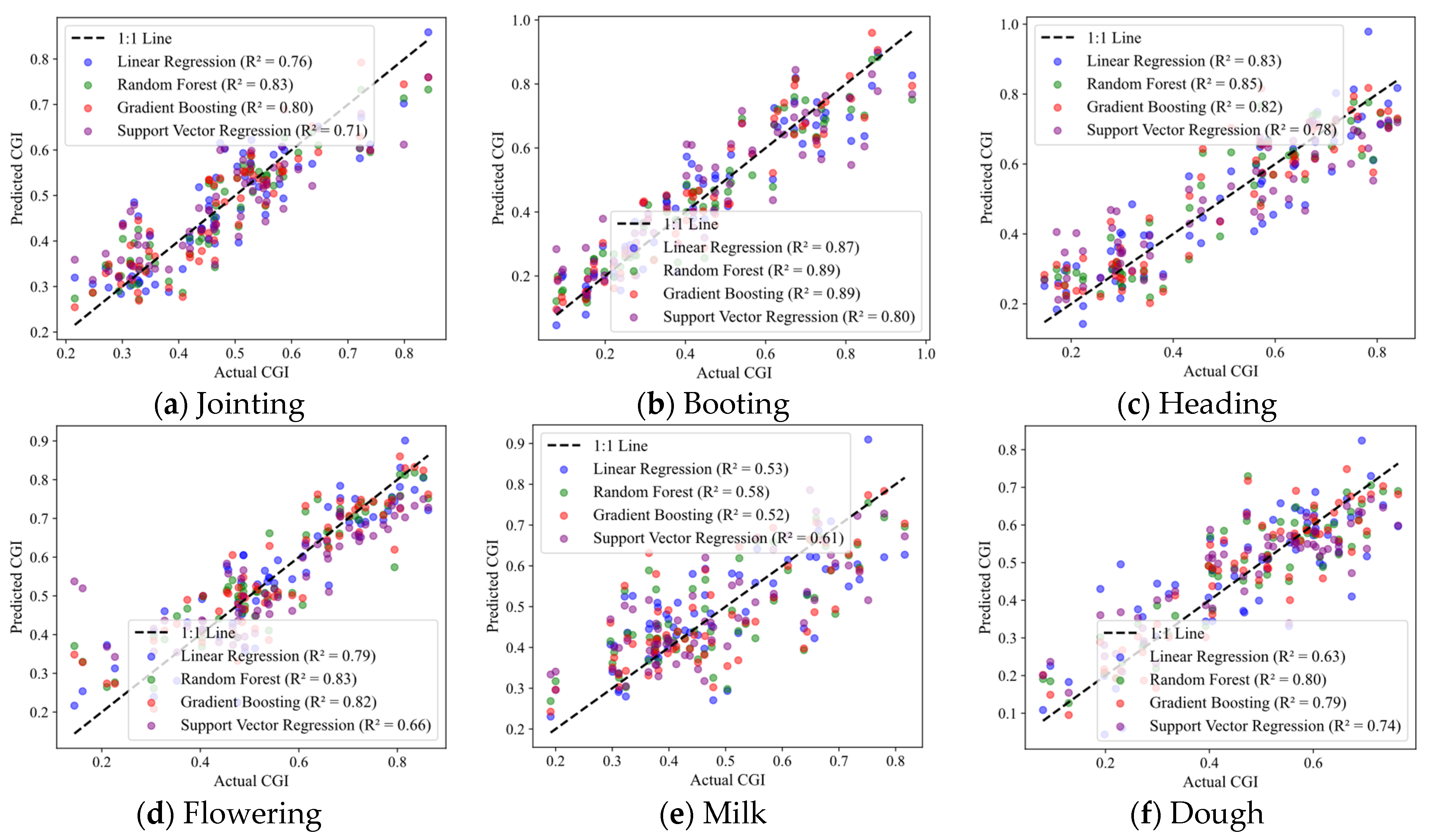
3.3.3. Results of the CGIac Inversion Model

Based on the above feature selection results, winter wheat CGIac inversion models were constructed for different growth stages using linear regression (LR) and nonlinear regression models (RF, GB, and SVR). First, the selected feature data were subjected to 10-fold cross-validation [46], with all samples randomly divided into 80% for the training set and 20% for the test set. The accuracy of the inversion models is shown in

Table 7. Accuracy analysis of CGI inversion at different growth stages.

Growth Stages	LR		RF		GB		SVR
	R2	RMSE	R2	RMSE	R2	RMSE	R2	RMSE
Jointing	0.759	0.0045	0.827	0.0032	0.803	0.0037	0.710	0.0054
Booting	0.869	0.0072	0.895	0.0058	0.891	0.0060	0.802	0.0109
Heading	0.830	0.0074	0.851	0.0066	0.823	0.0078	0.784	0.0094
Flowering	0.794	0.0063	0.831	0.0052	0.816	0.0056	0.663	0.0104
Milk	0.533	0.0103	0.581	0.0092	0.522	0.0105	0.613	0.0085
Dough	0.627	0.0111	0.801	0.0059	0.793	0.0062	0.738	0.0078

Note: Bold values denote best results.

, where the bolded values represent the best results. Figure 7 presents the corresponding inversion results for the comprehensive growth index of winter wheat at different growth stages.

Generally, the results indicate significant variation in inversion accuracy across the models and growth stages. RF delivered the best performance in most stages, achieving R² values of 0.827 and 0.895 in the jointing and booting stages, respectively, with low RMSE values. GB followed closely in terms of inversion accuracy, with the highest R² of 0.891 during the booting stage, closely approaching the precision of RF. In contrast, LR showed clear limitations when managing complex crop growth data, especially during the milk and dough stages, where the R² was as low as 0.533. The SVR model also performed poorly in the flowering and milk stages, with a lowest R² of 0.613. To provide a more intuitive visualization of the inversion results for different algorithms at each growth stage, Figure 7 shows the specific inversion results for the comprehensive growth monitoring index of winter wheat. In the figure, the points in the scatter plots for GB and RF models are closest to the diagonal, indicating higher prediction accuracy, with R² values approaching 1. In contrast, the scatterplots for LR and SVR show larger dispersion, reflecting lower R² values.

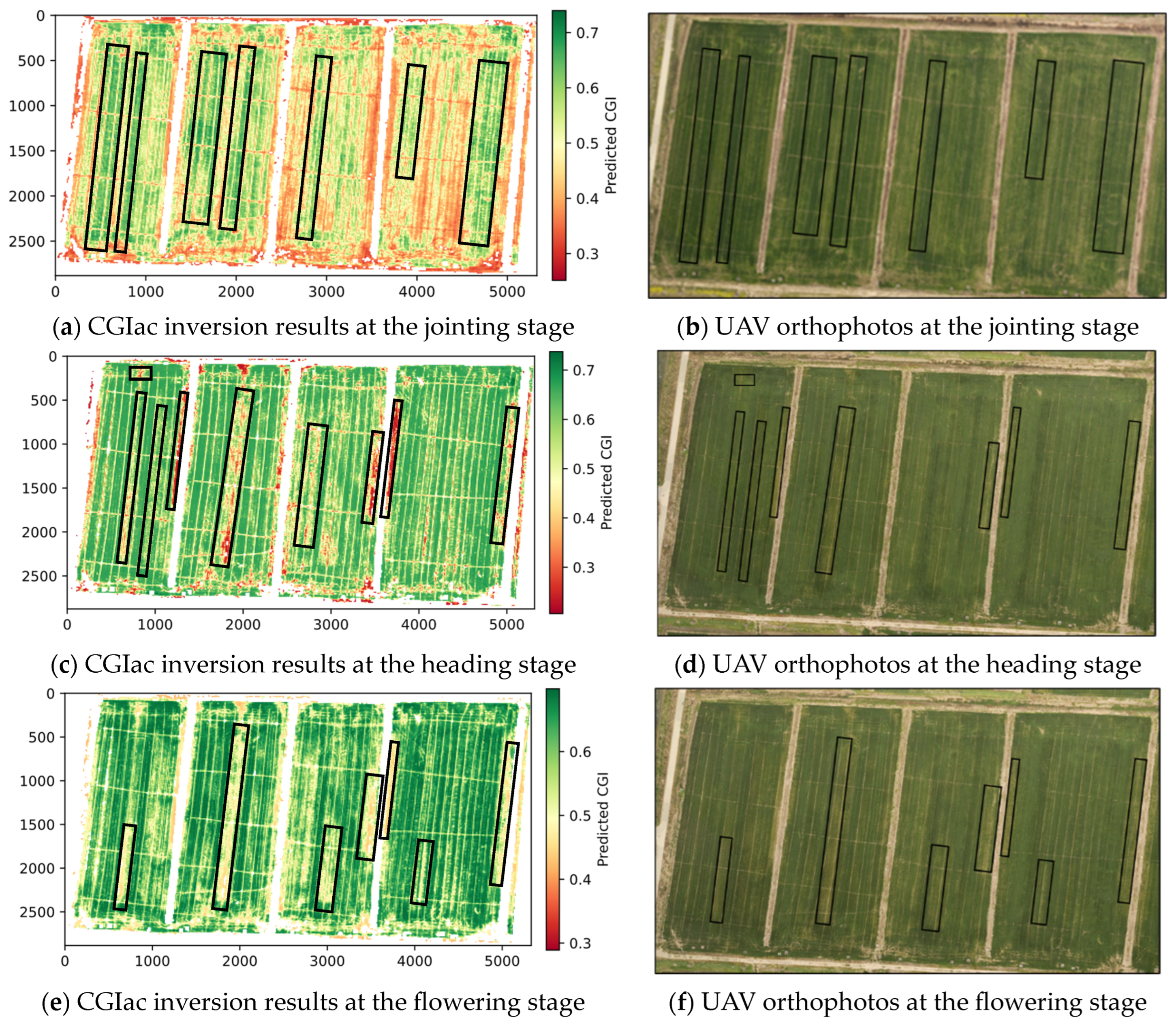
3.4. Application of the Optimal Inversion Model in Regional Growth Monitoring

Using the trained RF-based CGIac inversion model, we applied it to analyze winter wheat growth distribution across the entire study area, excluding the effects of ridges and roads. The result provided the growth distribution of winter wheat in the study region (see Figure 8). Figure 8a,c,e show the crop growth distribution during the jointing, heading, and flowering stages, respectively. The darker green areas represent regions of better growth, primarily located in the central parts of the fields or continuously cultivated areas. In contrast, the poorer growth areas (red or yellow) are mostly found along the field edges.

The analysis shows that areas with poorer growth were more prevalent during the jointing stage (Figure 8a), particularly at the field edges. By the heading stage (Figure 8c) and flowering stages (Figure 8e), as the crops matured, the overall growth conditions improved, with an increase in green areas and a reduction in red and yellow areas. This indicates that the growth of winter wheat improved steadily across different growth stages, although some regions remained growth limited.

A comparison with the orthophotos acquired at each growth stage (Figure 8b,d,f) reveals differences in growth conditions within the fields. The regions highlighted by rectangles indicate areas with substantial growth variability. The textures in these regions are consistent with the growth distribution observed in the inversion maps, where areas with poorer growth exhibit lighter or more uneven textures in the orthophotos.

The comparison between the inversion results and orthophotos indicates a high level of consistency, demonstrating that the CGIac inversion model accurately reflects winter wheat growth conditions. This model is particularly effective in identifying areas with significant growth variability during critical growth stages, providing valuable insights into field management.

4. Discussion

The focus of this study is to propose a novel method for constructing a CGI for winter wheat. This method combines various growth indicators, representing morphology, physiology, biochemistry, and yield potential, and evaluates their contribution to yield formation. The new comprehensive growth index, CGIac, is developed by applying an adaptive weighting method. Results demonstrate that LAI consistently contributes significantly to yield formation across all models, especially during the booting and heading stages [47]. LAI, a key agronomic parameter, is closely tied to wheat photosynthesis and transpiration and is widely used as a critical indicator of wheat growth and yield [48]. Starting from the heading stage, the weight of PH increases steadily, peaking at the flowering stage. PH is a critical indicator of crop structure, effectively reflecting crop growth [49]. During the flowering stage, the rapid increase in PH indicates vigorous wheat growth, which supports yield accumulation; however, during the later stages (dough stage), PH’s weight becomes negative. PWC directly reflects the crop’s water status, particularly during the jointing and booting stages, when sufficient water is vital for growth [50], leading to higher PWC weights during these periods. As the crop reaches maturity, excess or insufficient water can negatively affect yield, explaining why PWC’s weight declines or becomes negative in later stages. Furthermore, our analysis shows that the weight allocation of LAI, PH, and SPAD in the RF model is consistent with practical field management and crop growth knowledge.

Compared to individual growth indicators, the comprehensive growth index contains more detailed information about crop conditions and provides improved information representation [51]. To evaluate CGIac’s potential in winter wheat growth monitoring, we examined the impact of CGIac and individual growth parameters on yield correlation and prediction accuracy. The results showed that CGIac had stronger correlations with yield than any single growth indicator. A comparison of yield prediction accuracy with and without CGI features revealed that adding CGI significantly improved model performance to varying degrees. The inclusion of CGIac led to the highest increase in accuracy, up to 23.14%, followed by CGIcv and CGIav. That could be because CGIcv, constructed using the coefficient of variation method, can better allocate weights among growth indicators, especially when substantial differences exist. By contrast, CGIac integrates multiple individual indicators and considers each one’s contribution to yield, allowing it to capture the complex interactions between crop physiology and environmental conditions, thus improving model accuracy in predicting growth. Additionally, RF and GB models fully utilized the complex nonlinear relationships among different parameters, enhancing the models’ sensitivity to yield variations.

Analyzing the correlation between CGIac and VIs, we found that CGIac had a significant correlation with most VIs, consistent with previous research [14,15]. The flowering stage exhibited the highest correlations overall, with several VIs showing correlations greater than 0.8. This indicates that the flowering stage is a critical period for crop growth and yield prediction [43,52], because the VIs during this stage reflect crop physiological conditions and growth changes, forming significant linear relationships with CGIac. Although most indices still showed high correlations during the milk stage, some exhibited declines. This may be because these indices performed well in the early or middle growth stages (e.g., jointing and the booting stage) but could not accurately capture the crucial physiological changes during later growth stages, leading to reduced correlations. To enhance training speed, the Elastic Net method was used for feature selection, followed by inversion of CGIac using LR, RF, GB, and SVR models. The RF model performed best, with R² values consistently exceeding 0.8, particularly during the jointing stage (R² = 0.827) and booting stage (R² = 0.895), with RMSE values of 0.0032 and 0.0058, respectively. This is likely because the RF model excels at handling complex nonlinear relationships and effectively manages feature interactions in multi-feature datasets, reducing overfitting through its voting mechanism and ensuring model stability [53]. The GB model performed similarly to RF during most growth stages, especially during the booting stage (R² = 0.891), indicating strong performance. This success may be due to GB’s ability to iteratively optimize prediction errors, allowing it to manage nonlinear relationships effectively. However, its slower learning speed and tendency to overfit were reflected in its performance during the milk and dough stages. While LR performed adequately during early growth stages (e.g., jointing and booting), its accuracy dropped significantly during the milk and dough stages, as it struggled to handle nonlinear features, with R² dropping to 0.533 and RMSE increasing to 0.0103. The milk stage, representing a transitional phase between rapid growth and maturity, involves complex growth patterns that LR’s linear assumptions could not address effectively, resulting in poor prediction accuracy. Although SVR can handle nonlinear data, its performance in high-dimensional feature spaces was unstable, particularly during the flowering and milk stages, with R² values of 0.663 and 0.613, respectively. The kernel function in SVR may not have been sufficient to capture crop growth patterns effectively in complex datasets, revealing its limitations in handling detailed growth features.

Applying the optimal RF inversion model to winter wheat planting areas revealed significant growth variability during the jointing stage. This may be because the jointing stage marks the onset of rapid growth in wheat, making it particularly sensitive to environmental factors such as soil moisture, nutrient distribution, and sunlight. Additionally, the broadcast fertilization method led to uneven soil conditions, resulting in visible differences in wheat growth. As growth progressed, genetic traits became more influential, reducing growth variability during the heading and flowering stages. However, differences in soil fertility and terrain continued to cause variations in wheat growth in certain areas. Furthermore, comparing the orthophotos of winter wheat from the same period confirmed that the actual growth patterns closely matched the inversion results.

5. Conclusions

This paper comprehensively analyzes parameters that reflect the growth status of winter wheat, including SPAD, PH, LAI, BM, and PWC. Based on the differences in the contribution rates of individual growth parameters to yield, adaptive weight allocation was applied to each growth indicator, and a novel comprehensive growth index (CGIac) was proposed. This study first compares the correlations between CGIac (constructed with adaptive weights), CGIav (constructed with equal weights), CGIcv (constructed with the coefficient of variation method), and both individual growth parameters on yield. Then, these indices were added to four yield prediction models to evaluate the changes in prediction accuracy with and without CGI features. Finally, CGIac was inverted using spectral VIs, enabling the successful monitoring of winter wheat growth in the region. The conclusions are as follows:

The comparative analysis of the correlations between the three comprehensive growth indices (CGIac, CGIav, and CGIcv) and individual growth parameters with yield showed that the CGIac showed significantly higher correlations with yield than individual indicators, with most cases exhibiting highly significant correlations. Moreover, CGIac exhibited stronger correlations with yield compared to CGIcv and CGIav.

The analysis of incorporating CGI features into four yield prediction models revealed an improvement in prediction accuracy across all models. CGIac provided the most notable improvement, especially during critical growth stages like the flowering and milk stages, where it notably enhanced the performance of the RF and GB models. In contrast, the comprehensive indices CGIcv and CGIav, developed using the coefficient of variation and equal weight methods, showed suboptimal predictive performance in some growth stages.

The analysis of CGIac inversion results using the spectral vegetation index revealed that the RF model performed the best, particularly during the booting stage, with an R² value of 0.895 and an RMSE of 0.0058. The optimal inversion model, RF, was then applied to monitor winter wheat growth at the regional scale. A comparative analysis between the inversion results and the orthophotos of winter wheat growth during the same period showed a high level of consistency. This demonstrates that the inversion model can effectively reflect the growth status of winter wheat in the study area, providing valuable references for winter wheat field management.

References

1. Karmakar, P.; Teng, S.W.; Murshed, M.; Pang, S.; Li, Y.; Lin, H. Crop monitoring by multimodal remote sensing: A review. Remote Sens. Appl. Soc. Environ. 2024, 33, 101093. [Google Scholar] [CrossRef]
2. Wu, B.; Zhang, M.; Zeng, H.; Tian, F.; Potgieter, A.B.; Qin, X.; Yan, N.; Chang, S.; Zhao, Y.; Dong, Q.; et al. Challenges and Opportunities in Remote Sensing-Based Crop Monitoring: A Review. Natl. Sci. Rev. 2023, 10, nwac290. [Google Scholar] [CrossRef] [PubMed]
3. Wei, Z.; Fang, W. UV-NDVI for real-time crop health monitoring in vertical farms. Smart Agric. Technol. 2024, 8, 100462. [Google Scholar] [CrossRef]
4. Zhu, W.; Feng, Z.; Dai, S.; Zhang, P.; Wei, X. Using UAV multispectral remote sensing with appropriate spatial resolution and machine learning to monitor wheat scab. Agriculture 2022, 12, 1785. [Google Scholar] [CrossRef]
5. Ahmed, S.; Xin, H.; Faheem, M.; Qiu, B. Stability analysis of a sprayer uav with a liquid tank with different outer shapes and inner structures. Agriculture 2022, 12, 379. [Google Scholar] [CrossRef]
6. Ahmed, S.; Qiu, B.; Ahmad, F.; Kong, C.W.; Xin, H. A state-of-the-art analysis of obstacle avoidance methods from the perspective of an agricultural sprayer UAV’s operation scenario. Agronomy 2021, 11, 1069. [Google Scholar] [CrossRef]
7. Ahmed, S.; Qiu, B.; Kong, C.W.; Xin, H.; Ahmad, F.; Lin, J. A data-driven dynamic obstacle avoidance method for liquid-carrying plant protection UAVs. Agronomy 2022, 12, 873. [Google Scholar] [CrossRef]
8. Zhang, S.; Qiu, B.; Xue, X.; Sun, T.; Gu, W.; Zhou, F.; Sun, X. Effects of crop protection unmanned aerial system flight speed, height on effective spraying width, droplet deposition and penetration rate, and control effect analysis on wheat aphids, powdery mildew, and head blight. Appl. Sci. 2021, 11, 712. [Google Scholar] [CrossRef]
9. Memon, M.S.; Chen, S.; Niu, Y.; Zhou, W.; Elsherbiny, O.; Liang, R.; Du, Z.; Guo, X. Evaluating the Efficacy of Sentinel-2B and Landsat-8 for Estimating and Mapping Wheat Straw Cover in Rice–Wheat Fields. Agronomy 2023, 13, 2691. [Google Scholar] [CrossRef]
10. Olson, D.; Anderson, J. Review on unmanned aerial vehicles, remote sensors, imagery processing, and their applications in agriculture. Agron. J. 2021, 113, 971–992. [Google Scholar] [CrossRef]
11. Liu, X.; Wu, L.; Chen, L.; Ma, Y.; Li, T.; Wu, T. LAI inversion and growth evaluation of winter wheat using semi-empirical and semi-mechanistic modeling. Trans. Chin. Soc. Agric. Eng. 2024, 40, 162–170. [Google Scholar]
12. Wang, R.; Tuerxun, N.; Zheng, J. Improved estimation of SPAD values in walnut leaves by combining spectral, texture, and structural information from UAV-based multispectral image. Sci. Hortic. 2024, 328, 112940. [Google Scholar] [CrossRef]
13. Shu, M.; Li, Q.; Ghafoor, A.; Zhu, J.; Li, B.; Ma, Y. Using the plant height and canopy coverage to estimation maize aboveground biomass with UAV digital images. Eur. J. Agron. 2023, 151, 126957. [Google Scholar] [CrossRef]
14. Pei, H.; Feng, H.; Li, C.; Jin, X.; Li, Z.; Yang, G. Remote sensing monitoring of winter wheat growth with UAV based on comprehensive index. Trans. Chin. Soc. Agric. Eng. 2017, 33, 74–82. [Google Scholar]
15. Xu, Y.; Cheng, Q.; Wei, X.; Yang, B.; Xia, S.; Rui, T.; Zhang, S. Monitoring of winter wheat growth under UAV using variation coefficient method and optimized neural network. Trans. Chin. Soc. Agric. Eng. 2021, 37, 71–80. [Google Scholar]
16. El-Hendawy, S.; Al-Suhaibani, N.; Al-Ashkar, I.; Alotaibi, M.; Tahir, M.U.; Solieman, T.; Hassan, W.M. Combining genetic analysis and multivariate modeling to evaluate spectral reflectance indices as indirect selection tools in wheat breeding under water deficit stress conditions. Remote Sens. 2020, 12, 1480. [Google Scholar] [CrossRef]
17. Liu, H.; Zhang, F.; Zhang, L.; Lin, Y.; Wang, S.; Xie, Y. UNVI-based time series for vegetation discrimination using separability analysis and random forest classification. Remote Sens. 2020, 12, 529. [Google Scholar] [CrossRef]
18. Ouaadi, N.; Jarlan, L.; Ezzahar, J.; Zribi, M.; Khabba, S.; Bouras, E.; Bousbih, S.; Frison, P.L. Monitoring of wheat crops using the backscattering coefficient and the interferometric coherence derived from Sentinel-1 in semi-arid areas. Remote Sens. Environ. 2020, 251, 112050. [Google Scholar] [CrossRef]
19. Bannari, A.; Asalhi, H.; Teillet, P.M. Transformed difference vegetation index (TDVI) for vegetation cover mapping. In Proceedings of the IEEE International Geoscience and Remote Sensing Symposium, Toronto, ON, Canada, 24–28 June 2002; pp. 3053–3055. [Google Scholar] [CrossRef]
20. Burns, B.W.; Green, V.S.; Hashem, A.A.; Massey, J.H.; Shew, A.M.; Adviento-Borbe, M.A.A.; Milad, M. Determining nitrogen deficiencies for maize using various remote sensing indices. Precis. Agric. 2022, 23, 791–811. [Google Scholar] [CrossRef]
21. Gitelson, A.A.; Gritz, Y.; Merzlyak, M.N. Relationships between leaf chlorophyll content and spectral reflectance and algorithms for non-destructive chlorophyll assessment in higher plant leaves. J. Plant Physiol. 2003, 160, 271–282. [Google Scholar] [CrossRef]
22. Yan, K.; Gao, S.; Chi, H.; Qi, J.; Song, W.; Tong, Y.; Mu, X.; Yan, G. Evaluation of the vegetation-index-based dimidiate pixel model for fractional vegetation cover estimation. IEEE Trans. Geosci. Remote Sens. 2021, 60, 4400514. [Google Scholar] [CrossRef]
23. Sewiko, R.; Sagala, H.A.M.U. The use of drone and visible atmospherically resistant index (VARI) algorithm implementation in mangrove ecosystem health’s monitoring. Asian J. Aquat. Sci. 2022, 5, 322–329. [Google Scholar] [CrossRef]
24. Gitelson, A.A.; Viña, A.; Ciganda, V.; Rundquist, D.C.; Arkebauer, T.J. Remote estimation of canopy chlorophyll content in crops. Geophys. Res. Lett. 2005, 32, L08403. [Google Scholar] [CrossRef]
25. Liu, Y.; Sun, L.; Liu, B.; Wu, Y.; Ma, J.; Zhang, W.; Wang, B.; Chen, Z. Estimation of Winter Wheat Yield using multiple temporal vegetation indices derived from UAV-Based multispectral and hyperspectral imagery. Remote Sens. 2023, 15, 4800. [Google Scholar] [CrossRef]
26. Raper, T.B.; Varco, J.J. Canopy-scale wavelength and vegetative index sensitivities to cotton growth parameters and nitrogen status. Precis. Agric. 2015, 16, 62–76. [Google Scholar] [CrossRef]
27. Gitelson, A.A. Wide dynamic range vegetation index for remote quantification of biophysical characteristics of vegetation. J. Plant Physiol. 2004, 161, 165–173. [Google Scholar] [CrossRef]
28. Gamon, J.A.; Field, C.B.; Goulden, M.L.; Griffin, K.L.; Hartley, A.E.; Joel, G.; Penuelas, J.; Valentini, R. Relationships between NDVI, canopy structure, and photosynthesis in three Californian vegetation types. Ecol. Appl. 1995, 5, 28–41. [Google Scholar] [CrossRef]
29. Wu, C.; Niu, Z.; Tang, Q.; Huang, W. Estimating chlorophyll content from hyperspectral vegetation indices: Modeling and validation. Agric. For. Meteorol. 2008, 148, 1230–1241. [Google Scholar] [CrossRef]
30. Huete, A.R. A soil-adjusted vegetation index (SAVI). Remote Sens. Environ. 1988, 25, 295–309. [Google Scholar] [CrossRef]
31. Gong, P.; Pu, R.; Biging, G.S.; Larrieu, M.R. Estimation of forest leaf area index using vegetation indices derived from Hyperion hyperspectral data. IEEE Trans. Geosci. Remote Sens. 2003, 41, 1355–1362. [Google Scholar] [CrossRef]
32. Broge, N.H.; Leblanc, E. Comparing prediction power and stability of broadband and hyperspectral vegetation indices for estimation of green leaf area index and canopy chlorophyll density. Remote Sens. Environ. 2001, 76, 156–172. [Google Scholar] [CrossRef]
33. Tucker, C.J. Red and photographic infrared linear combinations for monitoring vegetation. Remote Sens. Environ. 1979, 8, 127–150. [Google Scholar] [CrossRef]
34. Ren, H.; Zhou, G. Determination of green aboveground biomass in desert steppe using litter-soil-adjusted vegetation index. Eur. J. Remote Sens. 2014, 47, 611–625. [Google Scholar] [CrossRef]
35. Sripada, R.P.; Heiniger, R.W.; White, J.G.; Meijer, A.D. Aerial color infrared photography for determining early in-season nitrogen requirements in corn. Agron. J. 2006, 98, 968–977. [Google Scholar] [CrossRef]
36. Mehrotra, S.; Kumar, A.; Roy, A. Classifying Pinus roxburghii Using an Innovative Training Approach of Fuzzy Models While Handling Heterogeneity Within Class in Western Himalayan Forests. J. Indian. Soc. Remote Sens. 2024, 52, 1269–1283. [Google Scholar] [CrossRef]
37. Gitelson, A.A.; Merzlyak, M.N. Remote estimation of chlorophyll content in higher plant leaves. Int. J. Remote Sens. 1997, 18, 2691–2697. [Google Scholar] [CrossRef]
38. Kim, Y.S. Comparison of the decision tree, artificial neural network, and linear regression methods based on the number and types of independent variables and sample size. Expert Syst. Appl. 2008, 34, 1227–1234. [Google Scholar] [CrossRef]
39. Belgiu, M.; Drăguţ, L. Random forest in remote sensing: A review of applications and future directions. ISPRS J. Photogramm. Remote Sens. 2016, 114, 24–31. [Google Scholar] [CrossRef]
40. Bentéjac, C.; Csörgő, A.; Martínez-Muñoz, G. A comparative analysis of gradient boosting algorithms. Artif. Intell. 2021, 54, 1937–1967. [Google Scholar] [CrossRef]
41. Awad, M.; Khanna, R.; Awad, M.; Khanna, R. Support vector regression. In Efficient Learning Machines; Springer: Berlin/Heidelberg, Germany, 2015; pp. 67–80. [Google Scholar] [CrossRef]
42. Patro, S.; Sahu, K.K. Normalization: A preprocessing stage. arXiv 2015, arXiv:1503.06462. [Google Scholar] [CrossRef]
43. Tao, H.; Xu, L.; Feng, H.; Yang, G.; Miao, M.; Lin, B. Monitoring of winter wheat growth based on UAV hyperspectral growth index. Trans. Chin. Soc. Agric. Mach. 2020, 51, 180–191. [Google Scholar] [CrossRef]
44. Zhang, H.; Shao, W.; Qiu, S.; Wang, J.; Wei, Z. Collaborative analysis on the marked ages of rice wines by electronic tongue and nose based on different feature data sets. Sensors 2020, 20, 1065. [Google Scholar] [CrossRef] [PubMed]
45. Zou, H.; Hastie, T. Regularization and variable selection via the elastic net. J. R. Stat. Soc. Ser. B 2005, 67, 301–320. [Google Scholar] [CrossRef]
46. Stone, M. Cross-validation: A review. Stat. J. Theor. Appl. Stat. 1978, 9, 127–139. [Google Scholar] [CrossRef]
47. Zhou, K.; Zhou, T.; Ding, F.; Ding, D.; Wu, W.; Yao, Z.; Liu, T.; Huo, Z.; Sun, C. Wheat LAI Estimation in Main Growth Period Based on UAV Images. J. Agric. Sci. Technol. 2021, 23, 89–97. Available online: https://www.nkdb.net/EN/10.13304/j.nykjdb.2019.0515 (accessed on 12 September 2024).
48. Brisco, B.; Brown, R.J.; Hirose, T.; McNairn, H.; Staenz, K. Precision Agriculture and the Role of Remote Sensing: A Review. Can. J. Remote Sens. 1998, 24, 315–327. [Google Scholar] [CrossRef]
49. Tilly, N.; Hoffmeister, D.; Cao, Q.; Huang, S.; Lenz-Wiedemann, V.; Miao, Y.; Bareth, G. Multitemporal crop surface models: Accurate plant height measurement and biomass estimation with terrestrial laser scanning in paddy rice. J. Appl. Remote Sens. 2014, 8, 083671. [Google Scholar] [CrossRef]
50. Quemada, C.; Pérez-Escudero, J.M.; Gonzalo, R.; Ederra, I.; Santesteban, L.G.; Torres, N.; Iriarte, J.C. Remote Sensing for Plant Water Content Monitoring: A Review. Remote Sens. 2021, 13, 2088. [Google Scholar] [CrossRef]
51. Tang, Y.; Zhou, Y.; Cheng, M.; Sun, C. Comprehensive Growth Index (CGI): A Comprehensive Indicator from UAV-Observed Data for Winter Wheat Growth Status Monitoring. Agronomy 2023, 13, 2883. [Google Scholar] [CrossRef]
52. Prasad, N.R.; Patel, N.R.; Danodia, A. Crop Yield Prediction in Cotton for Regional Level Using Random Forest Approach. Spat. Inf. Res. 2021, 29, 195–206. [Google Scholar] [CrossRef]
53. Biau, G. Analysis of a Random Forests Model. J. Mach. Learn. Res. 2012, 13, 1063–1095. [Google Scholar]
Figure 1. Study area in Zhenjiang City, Jiangsu Province. (a) the spatial distribution of sampling points in 2023; (b) the spatial distribution of sampling points in 2024.
Agriculture 14 01900 g001
Figure 2. Description of the growth and development of wheat at different growth stages.
Agriculture 14 01900 g002
Figure 3. Performance comparison of models.
Agriculture 14 01900 g003
Figure 4. Correlation between CGIac and yield constructed with different machine learning methods at different growth stages. (ad) show the correlation results between CGIac and yield for different models in 2023; (eh) show the correlation results between CGIac and yield for different models in 2024.
Agriculture 14 01900 g004aAgriculture 14 01900 g004b
Figure 5. Violin plots of sensitivity analysis of CGIac constructed by different machine learning methods and each single indicator in terms of yield correlation. (ad) denote the results of different CGIacs with the single indicator in 2023; (eh) denote the results of different CGIacs with the single indicator in 2024.
Agriculture 14 01900 g005
Figure 6. Comparison of the correlation between CGI and yield, constructed using the equal weight method (CGIav), the coefficient of variation method (CGIcv), and the yield contribution method (CGIac), respectively. (ac) show the correlation with yield based on the three methods in 2023, respectively. Similarly, (df) depict the correlation with yield in 2024 using the same methods, respectively.
Agriculture 14 01900 g006
Figure 7. The inversion results of CGIac for winter wheat at different growth stages.
Agriculture 14 01900 g007
Figure 8. Regional growth inversion of winter wheat at different growth stages. (a,c,e) show the inversion results of growth areas for the jointing, heading, and flowering stages, respectively, with (b,d,f) corresponding to the UAV orthophotos for the same stages.
Agriculture 14 01900 g008