Abstract
Considering the problems of high tillage resistance and high energy consumption in existing subsoiling shovels, the contour-fitting curve characteristics of the front paw toes of mole crickets were applied to the structural design of subsoiling shovels using bionic principles. Combined with the structure of an existing subsoiling shovel, three types of bionic subsoiling shovels were designed using bionic principles, aiming to reduce tillage resistance and energy consumption. In order to investigate their tillage effect, the microparameters of the red soil in South China were calibrated using EDEM 2020, and a corresponding discrete element soil model was established. The simulation conducted on the subsoiling process using both common and bionic subsoiling shovels, and the disturbance of the red soil by common and bionic subsoiling shovels, as well as the tillage resistance and kinetic energy experienced by subsoiling shovels, were studied. The results demonstrated that, compared with the common subsoiling shovel, the bionic subsoiling shovel 1 experienced a 5.31% reduction in tillage force, with a 4.01% reduction in tillage force at the shovel tip, a 7.15% reduction in tillage force at the shovel handle, and a 6.33% reduction in energy consumption. The bionic subsoiling shovel 2 experienced a 9.25% reduction in tillage force, with an 11.43% reduction in tillage force at the tip, a 5.49% reduction in tillage force at the handle, and a 10.58% reduction in energy consumption. The bionic subsoiling shovel 3 experienced a 6.55% reduction in tillage force, with a 5.87% reduction in tillage force at the tip and a 7.72% reduction in tillage force at the handle. Further verification has shown that the bionic subsoiling shovel has better resistance reduction and energy reduction effects.
1. Introduction
Arable land is vital for crop growth and human survival. However, due to population growth and rapid rural urbanization, the availability of arable land is shrinking. The frequent action of traditional machines and long-term unreasonable tillage methods also lead to the deterioration of soil structure and performance; the middle and deep soil is continuously compacted and evolves into a solid plow pan, which not only reduces soil fertility and permeability, but seriously affects soil quality, crop yield, and quality and overall agricultural productivity. To ensure the sustainable development of agriculture, it is urgent to maintain the quantity and quality of cultivated land.
There is soil erosion and water erosion in the topsoil layer due to long-term traditional tillage operations. This results in the loss of a large amount of water and organic matter in the soil, making the tillage layer shallower [1]. The repeated passage of tractors and agricultural implements often results in soil compaction. Soil compaction results in a decrease in porosity between soil aggregates [2]. Soil compaction can limit the growth and development of crop roots, affecting the growth status of crops [3]. Statistics reveal substantial economic losses due to soil compaction, with estimates indicating annual crop production losses of up to USD 1 billion in the United States and USD 144 million in a single agricultural region in Australia [4,5]. China is also facing this challenge, with 66% of farmland having thin plow layers and 26% of locations having excessive soil bulk density [6]. The agricultural mechanization rate in Heilongjiang Province, China is at a relatively high level nationwide. The increase in the weight and strength of agricultural machinery has led to an increase in soil compaction and a decrease in soil productivity in Heilongjiang Province’s farmland [7].
In this context, the international community has proposed conservation tillage based on the principle of no or minimum tillage. Subsoiling technology is one of the four key technologies of conservation tillage. It employs subsoiling shovels to break up the soil, disrupting the compacted subsoil layer and enhancing the depth of tillage without inverting the soil. Subsoiling technology helps to restore soil vitality, improves soil structure, and enhances soil water retention capacity, thereby enhancing arable land quality and overall productivity.
Subsoiling operations are currently widely recognized as an effective method to mitigate soil compaction issues [8]. However, the subsoiling device generally has disadvantages such as high tillage resistance and high energy consumption during the operation. The subsoiling shovel, as the pivotal component of the subsoiling implement, is also the main source of resistance in subsoiling operations. Hence, optimizing the subsoiling shovel’s structure to reduce resistance and energy consumption has become a crucial area of research [9,10].
Decreasing tillage resistance not only enhances the efficiency of subsoiling operations but also lowers the energy consumption of the implement and wear of machinery [11]. Currently, resistance reduction methods for subsoiling devices primarily involve vibration, coating, and structural approaches. Structural resistance reduction optimizes the subsoiling shovel design and key parameters of the handle and tip to achieve the goal of reducing resistance [12]. For example, Zhang Xirui et al. [13] developed a slant-handle folding subsoiling shovel that effectively reduces tillage resistance, allows for less ground surface disruption, and enhances soil-loosening efficiency.
The existing organisms in nature have gradually evolved into structures and forms that are highly adapted to the natural environment during the long-term process of survival of the fittest and are almost perfect. Biomimetics is committed to extracting information from organisms and applying it to the optimization of engineering problems. In recent years, with the robust advancement of bionics, numerous scholars have applied engineering bionic technology to the design of the shape of agricultural machinery’s soil contact components, making important contributions to reducing the working resistance of agricultural machinery’s soil contact components. While foreign research on bionics applied to agricultural machinery is relatively scarce, many Chinese scholars have actively explored and implemented bionic approaches to address engineering challenges in agricultural machinery.
Wei Song et al. [14] combined the structure of mole claws with a standard subsoiling device, employing EDEM for simulation and analysis, validated by a soil model test and field tests. The research results indicate that bionic subsoiling implements effectively enhance the plow-pan-soil-crushing capability and improve soil tillage quality. Jianfeng Sun et al. [15] designed a new type of furrow opener inspired by a bear claw structure, establishing an EDEM simulation model to study its interaction with red soil and assess the impact of tillage speed on energy consumption. Their results indicated lower power requirements and specific energy consumption for the bionic furrow opener compared to traditional furrowing blades. Wang et al. [4] utilized the ridge structure from shark scales in the design of a bionic subsoiling shovel, confirming superior performance in rent reduction and energy consumption over ordinary subsoiling shovels through discrete element simulations and field tests.
Currently, the development of subsoiling devices primarily relies on experimental methods, involving field tests and soil-trough tests to analyze the impact of structural and operational parameters on subsoiling energy consumption and effectiveness. While data from these tests are reliable, conducting large-scale, high-precision parameter optimization tests is challenging due to the high costs and seasonal nature of subsoiling operations, which also require substantial manpower and material resources [16]. The invisibility of the test process makes it challenging to observe and collect the actual trajectory and action state of the subsoiling device on the soil structure, as well as physical data of soil particles, hindering in-depth study of the subsoiling device’s consumption reduction mechanism [12]. As computer performance continues to improve, digital simulation technology has rapidly developed, offering an efficient means for parameter optimization analysis [17]. EDEM software, utilizing the discrete element algorithm, excels in simulating the dynamic characteristics of soil particles under stress conditions [18].
This study utilizes the discrete element method based on EDEM to simulate the interaction between the subsoiling shovel and soil. The discrete element method establishes an engineering model of tiny particles, simulating their motion under external forces and capturing changes in their properties kinematically and dynamically. It allows for the formation and breakage of contacts between particulate materials, effectively simulating both microscopic and macroscopic behaviors of particles. During the interaction of soil-touching components of agricultural machinery with soil, particles undergo dynamic rupture and flow; through appropriate contact model and discrete element parameters, this method effectively simulates soil–component interactions, aiding in the optimal design of agricultural machinery [11].
Zhiwei Zeng et al. [19] developed a discrete-element-method-based soil–tool–residue interaction model to explore interactions between various chisel tillage tools, soil, and residue, validating their model through soil tests. Chris Saunders et al. [20] employed the discrete element method to assess skimmer performance in field conditions, predicting tillage and traction forces. Chengguan Hang et al. [21] utilized the discrete element method to construct a soil model and investigate how tine spacing of subsoiling shovels affects soil disturbance. Fang et al. [22] studied and analyzed the interactions between straw, soil, and rotating bodies using the discrete element simulation method. Ying Chen et al. [23] established a discrete element model for the interaction between grouting tools and soil, and used spherical particles with viscous damping to simulate agricultural soil aggregates and their viscous behavior. The model was compared with measured values, with an error of less than 10%. Korn é l Tam á s et al. [24] simulated triaxial compression tests and direct shear tests based on DEM, and compared the results with soil box tests, verifying that DEM can effectively simulate the interaction between deep loose soil and soil. Jiyu Sun et al. [25] used a discrete element model (DEM) to simulate and analyze the interaction between biomimetic deep loosening and ordinary deep loosening (O-S) with soil, providing a basis for the design of a new type of drag-reducing and disturbance-reducing deep loosening. Many studies have shown that using smaller-radius spherical particles to model soil particle models can yield accurate simulation results, but setting the particle radius too small significantly increases computational cost. Wang et al. [26] used 10 mm spherical particles and established a reliable soil model.
This study aims to achieve the following:
- model the bionic subsoiling shovel;
- create a discrete element simulation model of interactions between subsoiling components and soil;
- simulate and compare tillage performance between common and bionic subsoiling shovels.
2. Materials and Methods
2.1. Design of Bionic Subsoiling Shovel
2.1.1. Selection of Bionic Objects
Bionics, as a discipline that studies biological structure and function to solve engineering and technological problems, plays a crucial role in advancing scientific development and technological progress. Soil-dwelling animals, after a long period of evolution, have developed superior abilities to obtain low cutting resistance and excellent soil removal and resistance reduction functions during excavation. This biological inspiration offers valuable insights for designing high-performance agricultural implements. Thus, applying bionic principles from animal paws and toes to the structural design of subsoiling shovels is expected to pave the way for achieving more efficient and low-resistance subsoiling operations.
The mole cricket, an insect order characterized by a cylindrical body ranging from 3 to 5 cm in length, primarily inhabits subterranean environments with loose, moist soil. They possess robust forefeet adept at soil excavation, enabling swift tunneling and burrowing. Many studies have shown that the forepaw toes of mole crickets have a strong ability to cut and break soil [27], and expand the soil while excavating, greatly improving excavation efficiency [28]. Gao et al. [29] utilized the contour curve of the largest claw toe from mole cricket forefeet in the design of excavator bucket teeth.
2.1.2. Optimization Design of Subsoiling Shovel Based on Bionic Structure
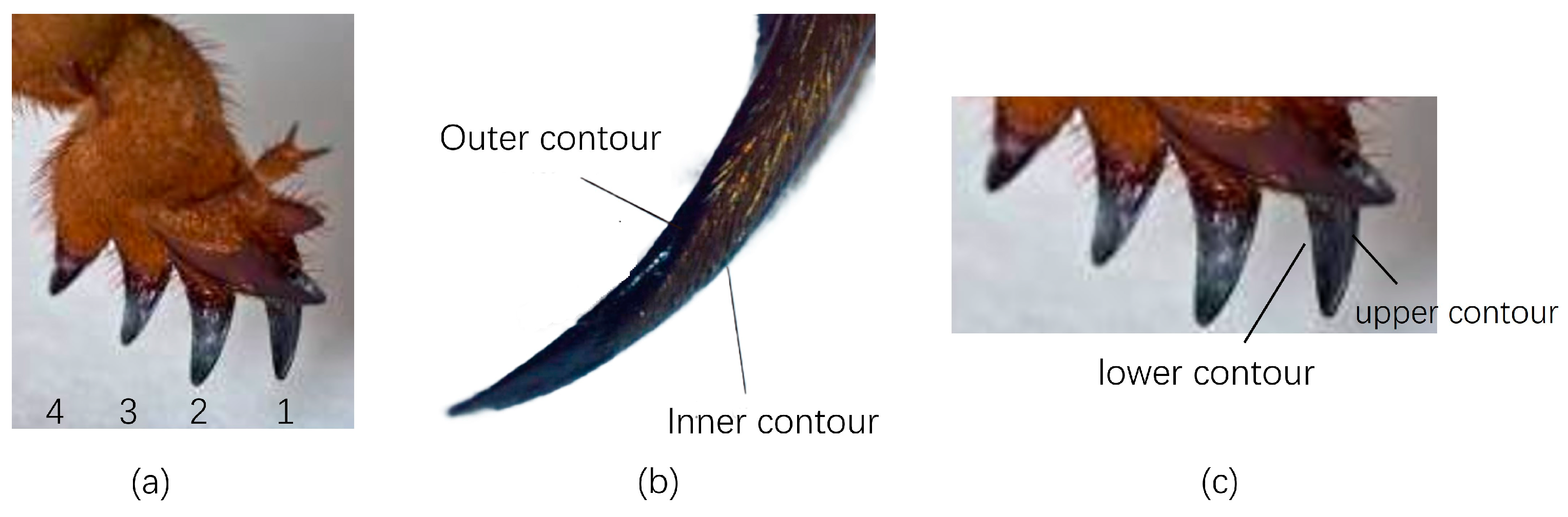
The front foot of the mole cricket has a total of four claw toes, as shown in Figure 1a. This study takes the four toes as the research object, extracts its longitudinal and cross-sectional profiles, as shown in Figure 1b,c, and refers to the structure of a common subsoiling shovel (abbreviated as CS) to design a bionic subsoiling shovel (abbreviated as BS), where toes 1, 2, 3, and 4 correspond to bionic subsoiling shovels 1, 2, 3, and 4, respectively.

Figure 1.
Claw toes and longitudinal and transverse sections of the forefoot of a mole cricket: (a) four toes of the forefoot of a mole cricket; (b) longitudinal section (Gao, 2009) [29]; (c) cross-section.
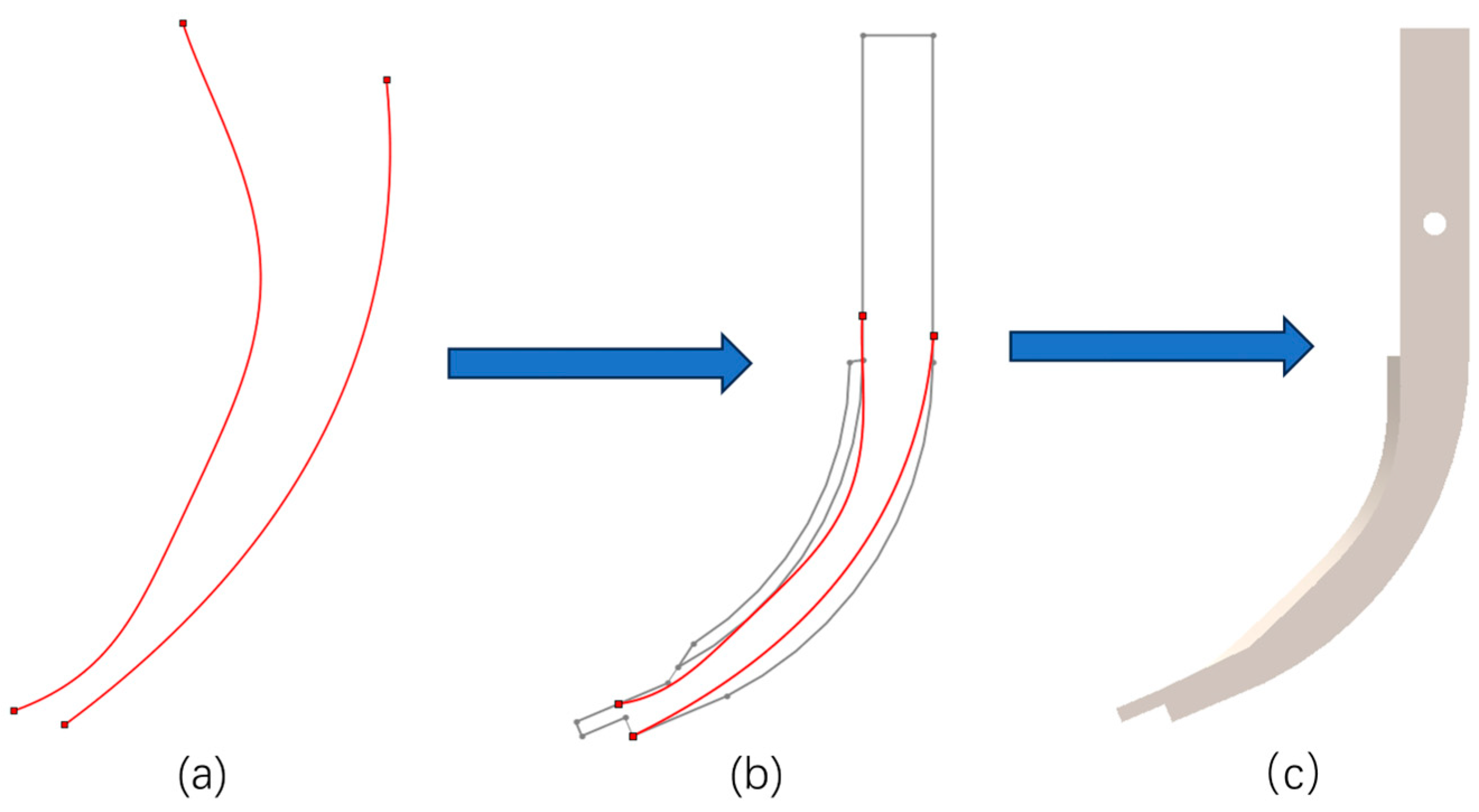
The inner and outer contour function expressions from the longitudinal section of the four toes of the mole cricket forefoot were imported into SolidWorks 2020, as detailed in Table 1 and Table 2 [30,31], to generate sketches of their inner and outer contour curves. For the purpose of comparing the bionic subsoiling shovel with the common subsoiling shovel, these sketches underwent preprocessing in CAD 2020, involving the scaling and rotation of the inner and outer contour curves, respectively. While ensuring that the overall dimensions of the two are approximately the same, the contour curve of the mole cricket claw toe replaced the contour curve of the operating part of the common subsoiling shovel. After processing, it was reintroduced into SolidWorks 2020 for tensile modeling to ultimately obtain the contour curve of the bionic shovel handle. The process of establishing the shovel handle of the bionic subsoiling shovel 1 is shown in Figure 2.

Table 1.
Parameters of polynomial equations for the fitting equations of the inner contour line in the longitudinal section of the claw toes of the anterior foot of the mole cricket.
Table 2.
Parameters of polynomial equations for the fitting equations of the outer contour line in the longitudinal section of the claw toes of the anterior foot of the mole cricket.
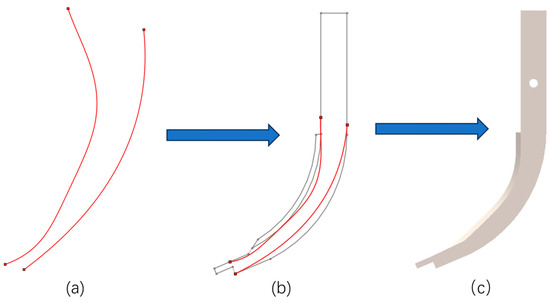
Figure 2.
Process of building the bionic subsoiling shovel 1 shovel handle: (a) contour curve of the anterior toe 1 of the mole cricket; (b) establishment process of the biomimetic subsoiling shovel 1 handle; (c) side view of the bionic subsoiling shovel 1 shovel handle.
As mole crickets primarily use the lower part of their claw toes for digging, which is chiefly responsible for cutting the soil, the lower contour function expressions of the claw toes of the four toes of the mole cricket’s forefeet in cross-section were imported into SolidWorks 2020, as shown in Table 3 [30]. The lower contour curve of the claw toe was symmetrically processed to obtain a sketch of the bionic curve, as shown in Figure 3, and the rest of the process is similar to that of the shovel handle. The front view of the bionic shovel tip is shown in Figure 4.
Table 3.
Parameters of polynomial equations for the fitting equations of the lower contour line in the cross-section of the claw toes of the anterior foot of the mole cricket.
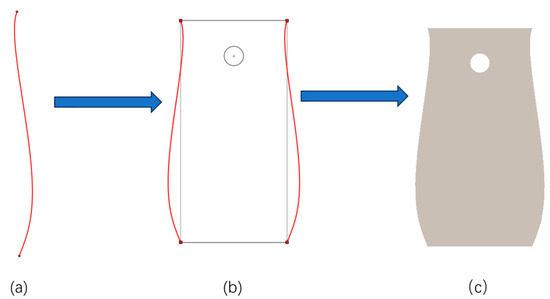
Figure 3.
Process of building the bionic subsoiling shovel 1 shovel tip: (a) lower contour curve of the anterior toe 1 cross-section of the mole cricket; (b) establishment process of the biomimetic subsoiling shovel 1 tip; (c) side view of the bionic subsoiling shovel 1 shovel tip.
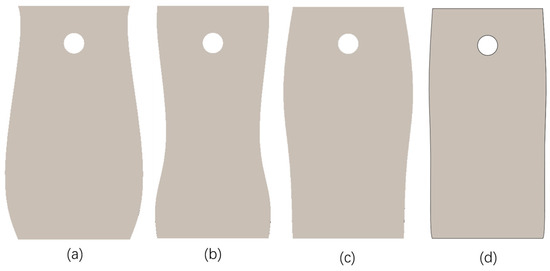
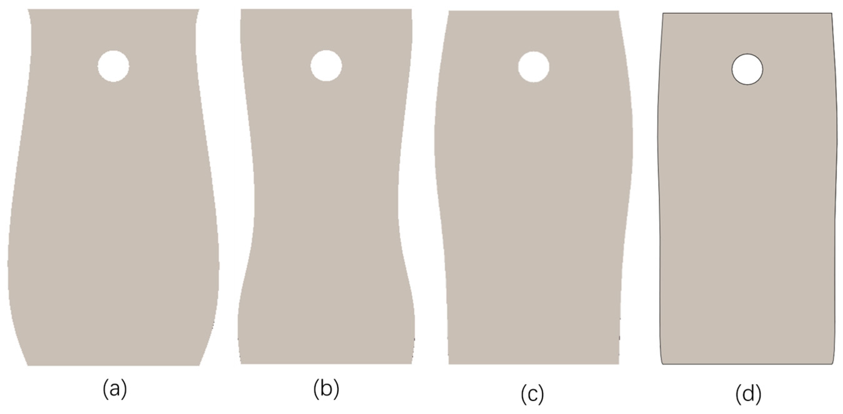
Figure 4.
Front view of common shovel tip and bionic shovel tip: (a) bionic subsoiling shovel 1; (b) bionic subsoiling shovel 2; (c) bionic subsoiling shovel 3; (d) bionic subsoiling shovel 4.
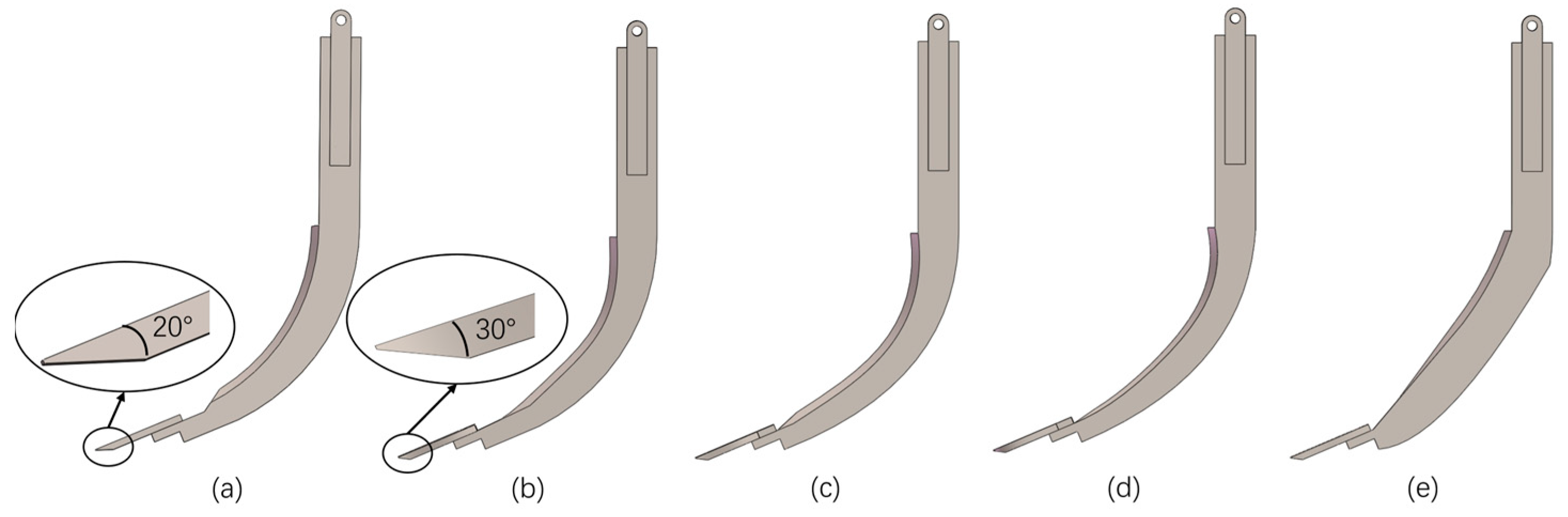
The end chamfer of the shovel tip was optimized from 20° to 30° by combining the tip portion of the claw toe from the mole cricket’s forefoot [18]. Finally, the shovel tip, shovel handle, and connecting parts were assembled to obtain the simplified side view of both the common subsoiling shovel and the bionic subsoiling shovel, as shown in Figure 5.
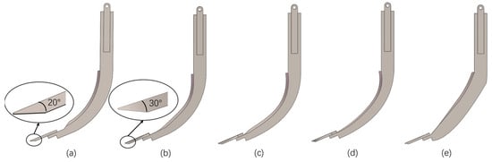
Figure 5.
Side view of common subsoiling shovel and bionic subsoiling shovel: (a) common subsoiling shovel; (b) bionic subsoiling shovel 1; (c) bionic subsoiling shovel 2; (d) bionic subsoiling shovel 3; (e) bionic subsoiling shovel 4.
2.2. Calibration of Discrete Element Simulation Parameters
2.2.1. Discrete Element Modeling
Analyzing the disturbance behavior of subsoiling soil forms the foundation for an in-depth study of the interaction law between the subsoiling shovel and soil. this paper conducts a simulation test on the interaction between the subsoiling shovel and soil using EDEM 2020. To reduce computational cost while ensuring simulation accuracy, this paper sets the minimum radius of the soil particle model to 6 mm spherical particles.
Considering the dimensions of the subsoiling shovel and the simulation calculation volume, the length, width, and height of the soil bin were determined to be 1300 mm × 800 mm × 500 mm, with the material parameters of both the soil bin and the subsoiling shovel set to 65Mn steel. When establishing the soil model, it is necessary to combine experiments and calculations to obtain the microscopic parameters for the discrete element simulation, consider agronomic factors, and comprehensively evaluate soil particle morphology and contact types between particles. Given the differences in the soil characteristics between the plow pan layer and the tillage layer, it was chosen to model the plow pan layer and tillage layer soil separately.
With respect to the red soil in South China, based on the measurement results, the soil moisture content is about 15.9%, and the thickness of the soil tillage layer was found to be between 15 and 20 cm, while the plow pan layer was about 18 cm below the surface. The soil in the tillage layer is relatively loose, with high water content and high viscosity. Therefore, the Hertz–Mindlin with JKR contact model was used, considering the effect of bonding between wet particles on particle movement. This model is suitable for simulating material with obvious bonding and agglomeration due to electrostatic forces and moisture, with a thickness set to 18 cm. The soil in the plow pan layer has low water content, small porosity, and is highly compacted. Therefore, the Hertz–Mindlin with bonding contact model was used. The Hertz–Mindlin with bonding contact model is used to bond adjacent particles, allowing for a certain degree of normal and tangential displacement. The thickness of this layer is set to 12 cm. The thickness of the heart soil layer beneath it is set to 5 cm [11].
2.2.2. Selection of Microscopic Parameters for Discrete Element Simulation
The key to modeling soil is to consider the morphology of soil particles and discrete element simulation parameters. The physical parameters of the discrete element soil model include both material and contact parameters. Material parameters mainly include the density, Poisson’s ratio, and shear modulus of the soil and subsoiling shovel, while contact parameters include the recovery coefficient, static friction coefficient, and dynamic friction coefficient between soil particles and between the soil and subsoiling shovel.
The material parameters of the soil and subsoiling shovel used in this study are public data, and the specific parameters are shown in Table 4 [32]. The contact parameters of the soil are microscopic parameters that need to be calibrated based on their macroscopic characteristics. The microscopic parameters of the soil in the tillage layer are calibrated using a soil-stacking test.
Table 4.
Material parameters of soil and subsoiling shovel.
2.2.3. Calibration of Soil Microparameters in the Tillage Layer
The research group investigated soil samples from the tillage layer of the test field and conducted a soil-stacking test using the funnel method, ultimately obtaining an average value of 36.25° as the true accumulation angle.
Zhai [33] combined literature data and the GEMM-recommended values of the built-in discrete element model database in EDEM to determine the initial range of microparameters of the tillage layer soil model, as shown in Table 5. Through experiments, it was found that soil JKR surface energy (G) had the most significant effect on the soil accumulation angle, followed by soil–soil rolling friction factor (C), soil–soil collision recovery factor (A), and soil–soil static friction factor (B). Conversely, soil–65Mn collision recovery coefficient (D), soil–65Mn static friction factor (E), and soil–65Mn rolling friction factor (F) had no significant effect on the accumulation angle. Therefore, in subsequent tests, parameters D, E, and F, which do not significantly affect the accumulation angle, will be set to intermediate levels within their initial ranges: 0.35, 0.85, and 0.1, respectively. Parameters A, B, C, and G, which do affect the accumulation angle significantly, will be prioritized as the main experimental factors for multi-factor and multi-objective physical parameter calibration and optimization.
Table 5.
Initial range of microparameters of the tillage layer.
2.2.4. Steepest Climb Test
The steepest climb test was designed to identify the vicinity of the optimum value. Based on the initial range of significant parameters A, B, C, and G, divided into 11 data groups with a gradual increase in range, the simulated accumulation angles for each group were recorded, analyzed, and are shown in Table 6. As the contact parameter gradually increased, the relative error values between the simulated and real accumulation angles first decreased and then increased. Among them, the relative error of the accumulation angle corresponding to the contact parameter value at level No. 2 is the smallest, indicating that the optimal value is near level No. 2. To further narrow down the optimal interval, levels No. 1 and No. 3 are selected as the new lower and upper bounds, respectively, for use in subsequent tests.
Table 6.
Steepest climb test design options and results.
2.2.5. Model Regression and Optimization
A four-factor, three-level Box–Behnken test was designed based on soil accumulation angle as the response variable and A, B, C, and G as the test factors. The experimental plan and results are shown in Table 7.
Table 7.
Box–Behnken experimental design program and results.
A quadratic regression model between soil particle accumulation angle and four contact parameters was developed using Design-Expert.13, and the model was analyzed for errors. Its quadratic polynomial equation is the following:
The experimental results of the model were analyzed using regression ANOVA. The results in Table 8 show that the coefficient of determination of the regression model is 0.9622, indicating that the model explains approximately 96.22% of the experimental variance, demonstrating a high fit with the actual data. The coefficient of correction determination is 0.9245, indicating a strong correlation. The coefficient of variation CV is 5.94%, and the misfit term p is 0.1273, more than 0.05, indicating a small proportion of non-normal error in the resulting equation and a good relationship with the regression equation. The experimental precision is 17.545, indicating good model accuracy. In summary, the model is highly reliable and suitable for further analysis. The model P, less than 0.0001, indicates that the accumulation angle regression model is highly significant. Within the given range of experimental factor levels, C, G, and G2 have a significant impact on the accumulation angle, while other factors have no significant impact on the accumulation angle.
Table 8.
Box–Behnken design quadratic regression model analysis of variance.
2.2.6. Analysis of Regression Model Interaction Effects
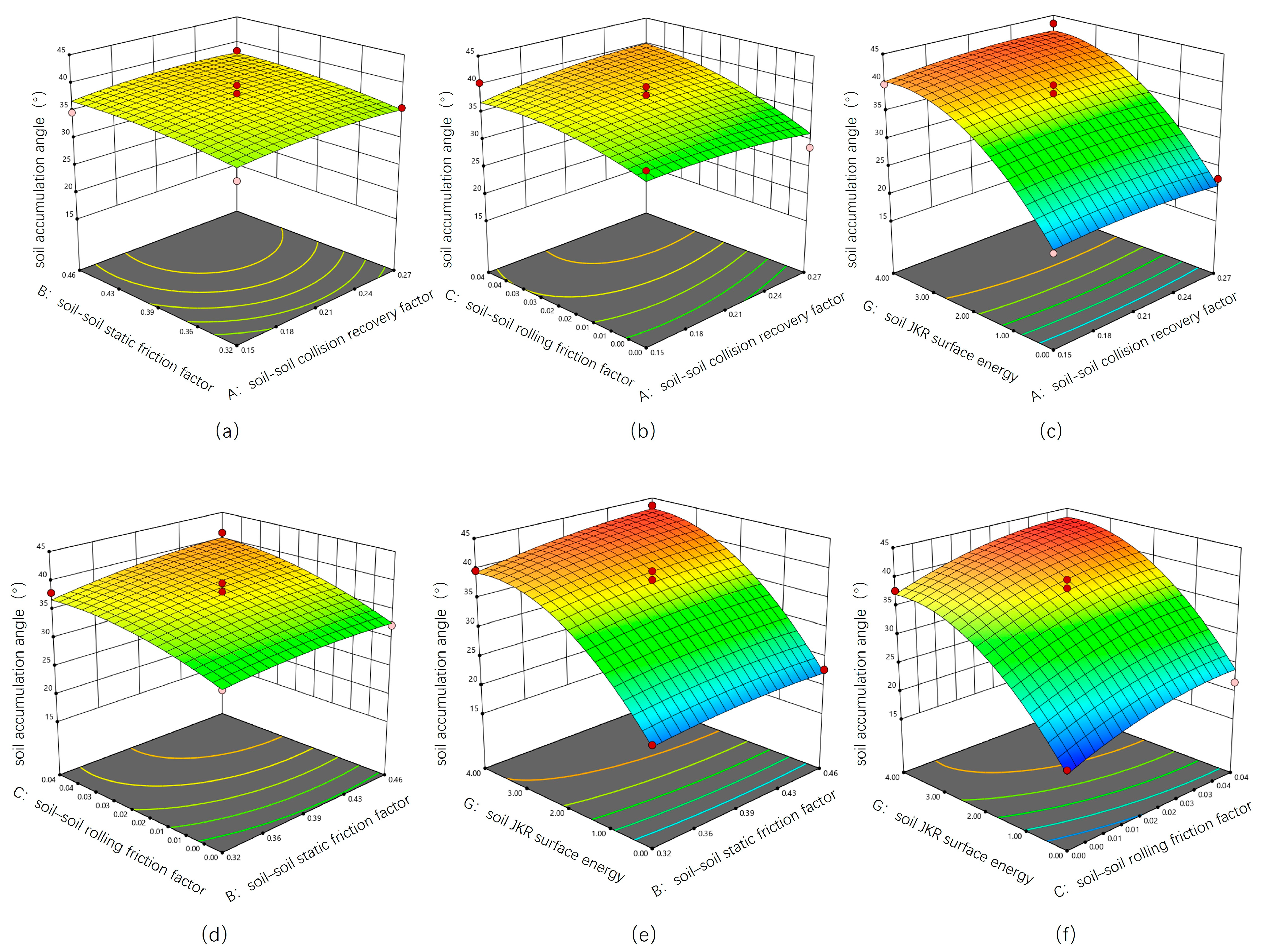
In this experiment, the soil accumulation angle was used as an evaluation index for the parameter calibration of the simulation model, and multiple regression was fitted to the model data using Design-Expert.13. The response surface of the generated interaction terms of various factors is shown in Figure 6.
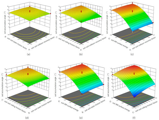
Figure 6.
Effect of interaction on soil accumulation angle: (a) A and B interaction, (b) A and C interaction, (c) A and G interaction, (d) B and C interaction, (e) B and G interaction, (f) C and G interaction.
Through further analysis of the interaction effects among various influencing factors on the response values, it can be observed from Figure 6a that the slope of the response surface does not change significantly, indicating that the changes in soil–soil collision recovery factor-A and soil–soil static friction factor-B have a relatively small impact on the accumulation angle. From Figure 6b, it can be seen that there is a certain change in the slope of the response surface. The response surface curve of soil–soil collision recovery factor-A does not change significantly, while the response surface curve of soil–soil rolling friction factor-C is steeper, indicating that C has a more significant impact on the accumulation angle. From Figure 6c, it can be seen that the slope of the response surface changes significantly, while the response surface curve of A does not change significantly; the response surface curve of soil JKR surface energy-G is steeper, indicating that G has a more significant impact on the accumulation angle. From Figure 6d, it can be seen that there is a certain change in the slope of the response surface, and the response surface curve of B does not change significantly, while the response surface curve of C is steeper, indicating that C has a more significant impact on the accumulation angle. From Figure 6e, it can be seen that the slope of the response surface changes significantly, while the response surface curve of B does not change much, and the response surface curve of G is steeper, indicating that G has a more significant impact on the accumulation angle. From Figure 6f, it can be seen that the slope of the surface changes significantly, indicating that C and G have a more significant impact on the stacking angle. The curvature of the contour lines in the figure is relatively flat, indicating that the interaction between various factors has no significant impact on the accumulation angle.
2.2.7. Parameter Optimization and Simulation Verification
Utilizing Design-Expert software, with a soil accumulation angle of 36.25° as the standard, multi-objective solution was performed on the parameter set of the quadratic regression model function values. A set of data was obtained: a soil–soil collision recovery factor of 0.27, a soil–soil static friction factor of 0.45, a soil–soil rolling friction factor of 0.01, and a soil JKR surface energy of 2.03 J/m3. The corresponding simulated accumulation angle was 36.56°, with a relative error of 0.8552% compared to the actual accumulation angle, indicating that the soil microparameters are basically consistent with the actual ones and can be applied to the dynamic analysis of relevant soil models. Figure 7 shows the comparison between actual and simulated stacking images, indicating that the soil model of the cultivated layer established using the obtained parameter set is accurate and reliable.
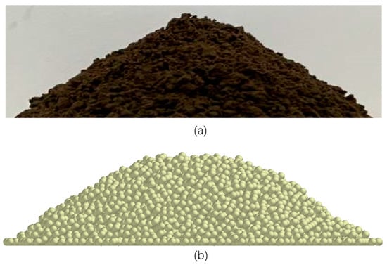
Figure 7.
Comparison of actual and simulated accumulation images: (a) actual accumulation angle image, (b) simulated accumulation angle image.
The relevant parameters of the plow subsoil were obtained from the study of Zhai [33]. The final established two-contact coupled discrete element soil model is shown in Table 9.
Table 9.
Soil model parameters.
2.3. Establishment of the Soil Bin Model
2.3.1. Modeling of the Plow Pan Soil
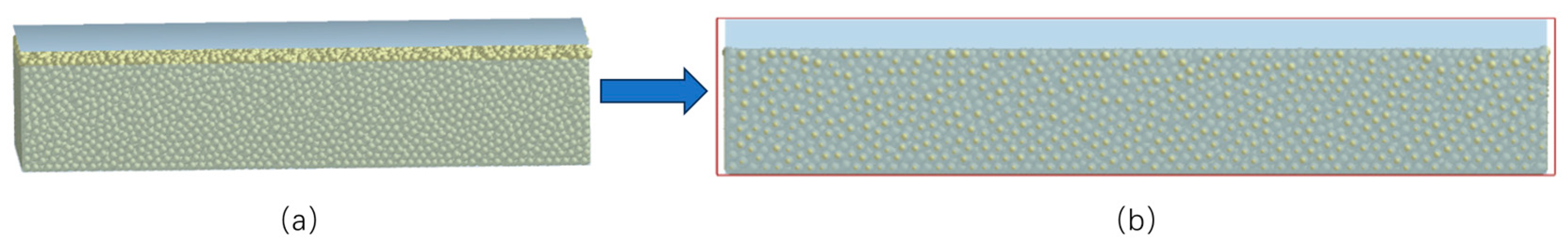
Due to the low moisture content, small porosity, and high degree of slaking in the plow pan soil, strong interparticle forces are present. Therefore, the Hertz–Mindlin model with bonding contacts was selected as the contact model for the plow subsoil. To simulate the plow subsoil more accurately, an extrusion plate was placed at the soil slot entrance. After a thickness of 20 cm is generated in the plow subsoil, the compression plate is controlled to move downwards by 3 cm, moderately compacting the subsoil, as depicted in Figure 8.
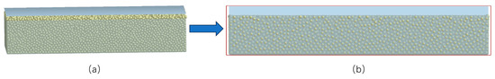
Figure 8.
Modeling of plow subsoil: (a) plow pan soil generation, (b) plow pan soil compression.
2.3.2. Modeling of Tillage Soil
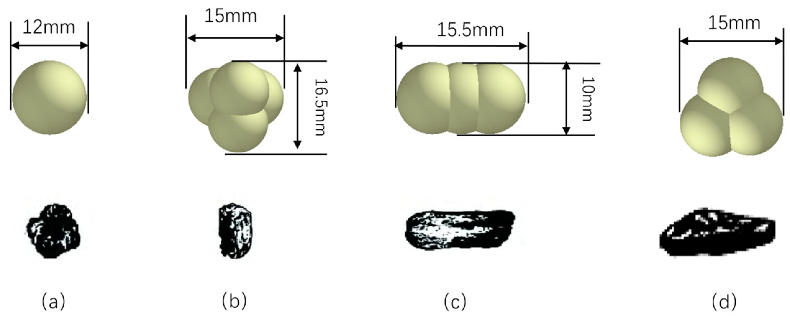
The tillage layer typically refers to the soil layer located 15–20 cm below the surface, characterized by loose texture and higher water content. The Hertz–Mindlin model with JKR contact was selected as the appropriate contact model for the tillage layer soil. Soil particles in the tillage layer often exhibit bulky, strip, flaky, and columnar appearances [34]. The shape of soil particles plays a crucial role in soil modeling. Therefore, in EDEM 2020, single spherical particles, a tetrahedral combination of four spherical particles, a linear combination of three spherical particles, and a triangular combination of three spherical particles were employed to simulate bulky, columnar, strip, and flaky soil particles in the actual tillage layer, depicted in Figure 9.
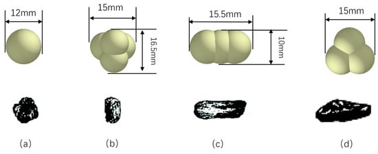
Figure 9.
Actual shape and model of soil particles: (a) bulky soil particles and their models, (b) columnar soil particles and their models, (c) strip soil particles and their models, (d) flaky soil particles and their models.
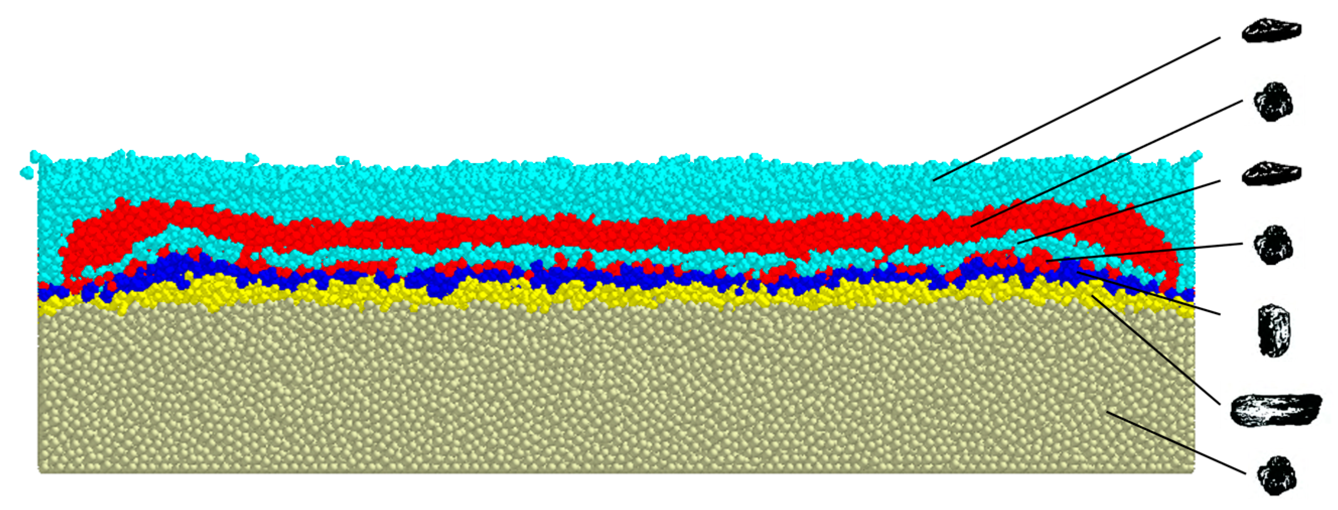
In view of the complexity and differences of the shape of soil particles in the tillage layer, the tillage layer was divided into six layers, and the shape of the particles from the surface to the inside were flaky, bulky, flaky, bulky, column, and strip, and the number of simulated soil particles is set based on the size of the simulated soil tank and the operating speed of the computer. The distribution of the soil particles in each layer is shown in Figure 10.
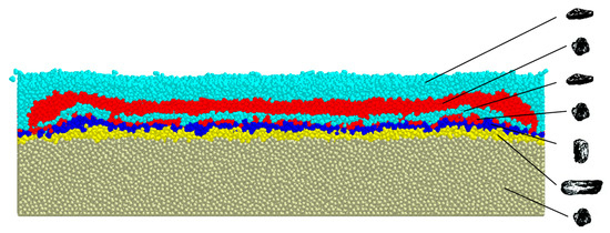
Figure 10.
Soil model.
3. Results and Discussion
3.1. Evaluation Indices of Tillage Performance
Tillage resistance is the main factor causing the increase in energy consumption of subsoiling machines and making it a critical index for evaluating its performance. Resistance data during the subsoiling process could be obtained quantitatively and intuitively using the EDEM post-processor, with its quantitative analysis index being the average value over one cycle. In addition, kinetic energy is also an important index that indirectly reflects the energy consumption of subsoiling machines. Through this method, the kinetic energy of all soil particles including both translational and rotational energies can be calculated, and its quantitative analysis index is also the average value within a cycle.
The motion module in EDEM can achieve simple movements; the geometric models of both the common and bionic subsoiling shovels were imported into EDEM 2020, and set the position relationship between virtual soil bin and subsoiling shovel based on actual working conditions. Based on the operational parameters of existing subsoiling machines, the forward speed of the subsoiling shovel was set at 0.83 m/s, with a plowing depth of 30 cm. Under these conditions, the subsoiling shovel traversed the soil model entirely within 2.1 s. Between 0.5 s and 1.5 s, the subsoiling shovel operated smoothly and continuously through the soil model without encountering boundary interference; therefore, data from 0.5 s to 1.5 s were selected for the study. These tillage performance indices will be analyzed qualitatively and quantitatively below.
3.2. Analysis of Tillage Resistance
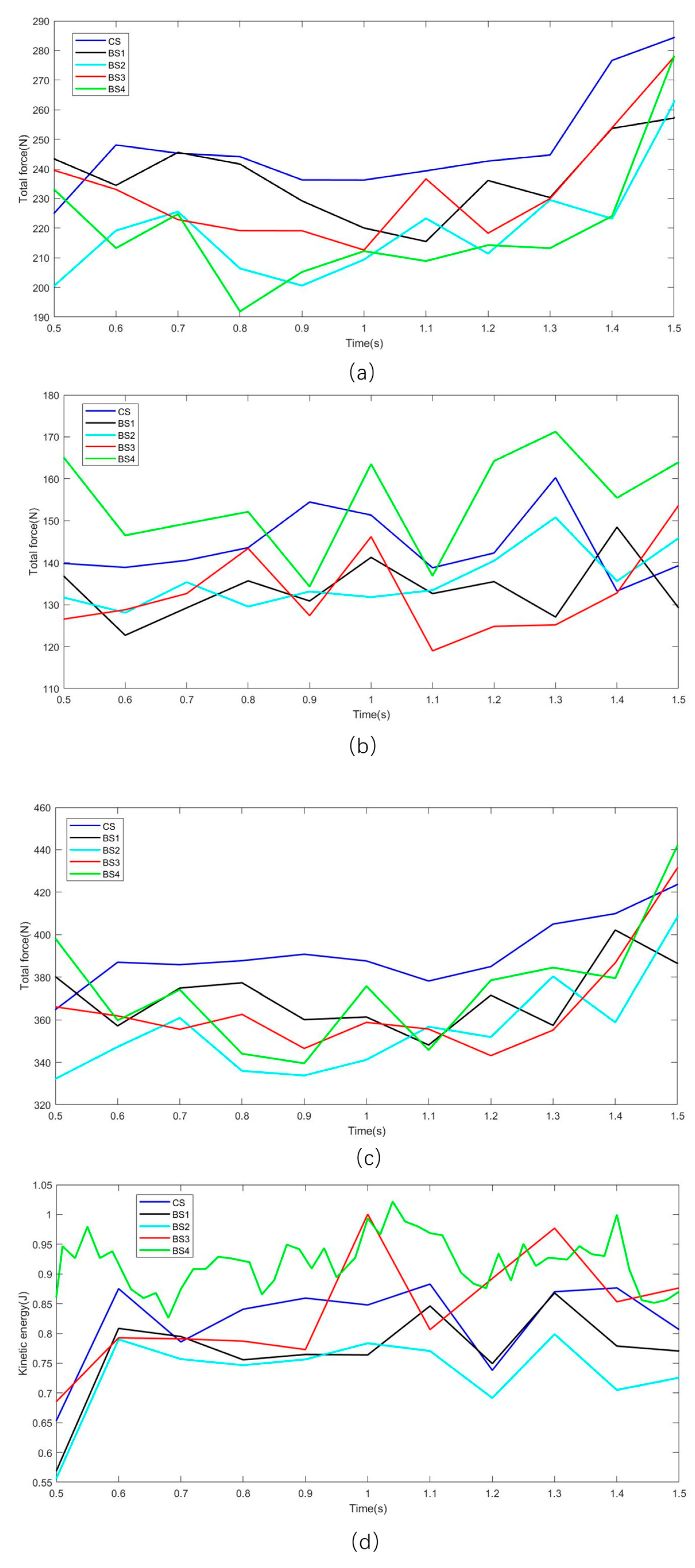
The images of the tillage resistance of soil particles subjected to common subsoiling shovels and bionic subsoiling shovels as a function of time are outputted in the EDEM 2020 post-processing interface, respectively, as shown in Figure 11a–c.
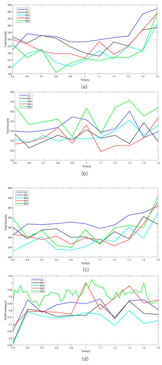
Figure 11.
Tillage performance variation curve: (a) tillage resistance to the shovel tip, (b) tillage resistance to the shovel handle, (c) total tillage resistance to the subsoiling shovel, (d) kinetic energy.
The subsoiling shovel mainly resists the squeezing force and friction force from the soil. From Figure 11, the total tillage resistance curve of the subsoiling shovel is slightly smoother than that of the individual subsoiling components. The tillage resistance curve of the shovel handle fluctuates greatly, which may be due to the fact that the tillage resistance mainly acts on the front shovel surface, and the force area of the shovel handle is large. It can be seen that the tillage resistance experienced by the bionic subsoiling shovel is significantly lower than that of the common subsoiling shovel. Except for the handle of BS4, the tillage resistance experienced by other bionic components are lower than that of the common subsoiling shovel components.
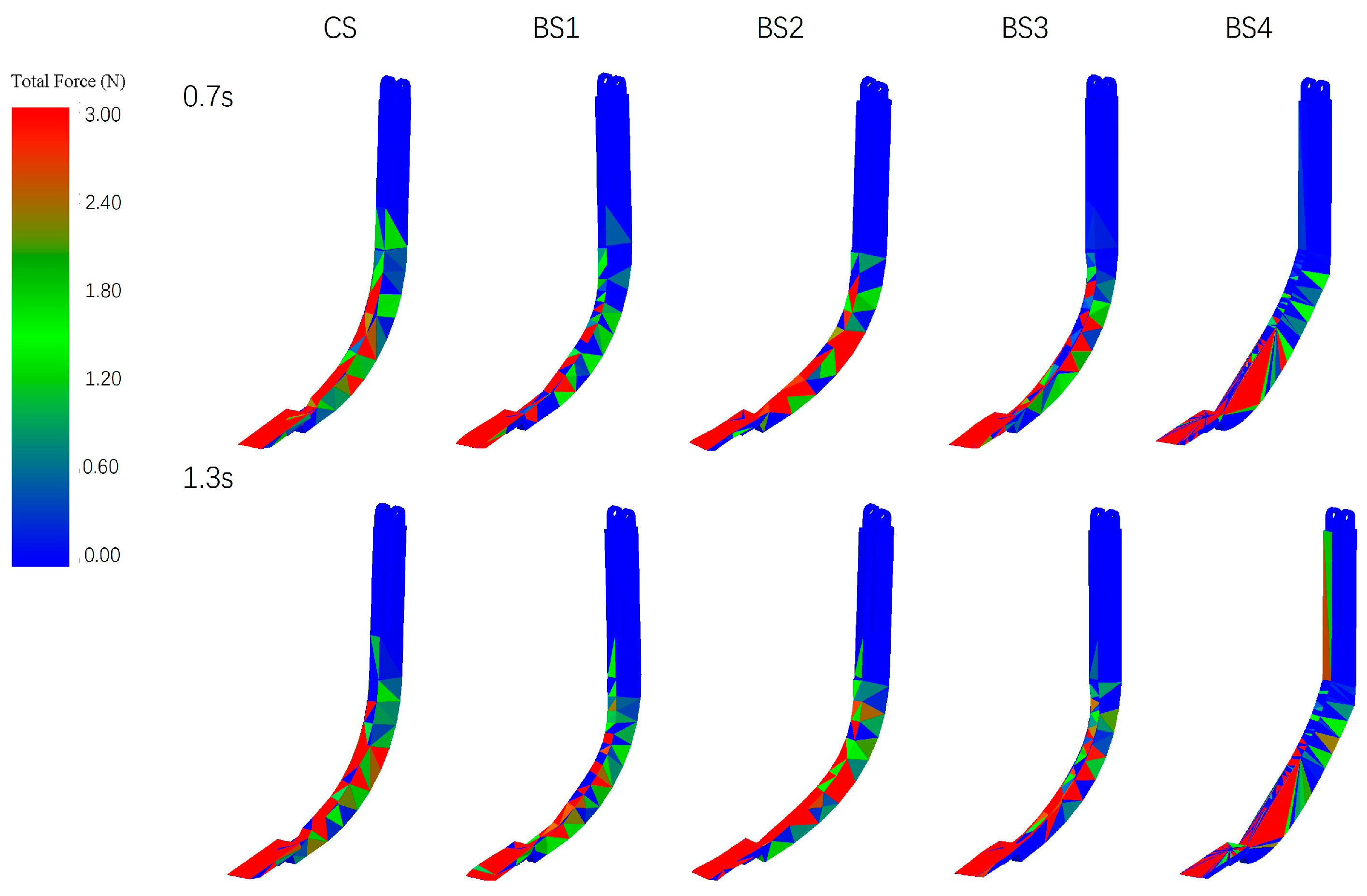
Further visual analysis of the tillage resistance on five types of subsoiling shovels was conducted on the EDEM 2020 post-processing interface. Take the cloud maps of the tillage forces acting on five types of subsoiling shovels at 0.7 s and 1.3 s, respectively, to represent the force situation during stable operation, as shown in Figure 12. The color represents the magnitude of the tillage force acting on the subsoiling shovel, with red representing the maximum force, followed by green, and blue the minimum.

Figure 12.
Visualization of force cloud for common subsoiling shovel and bionic subsoiling shovel.
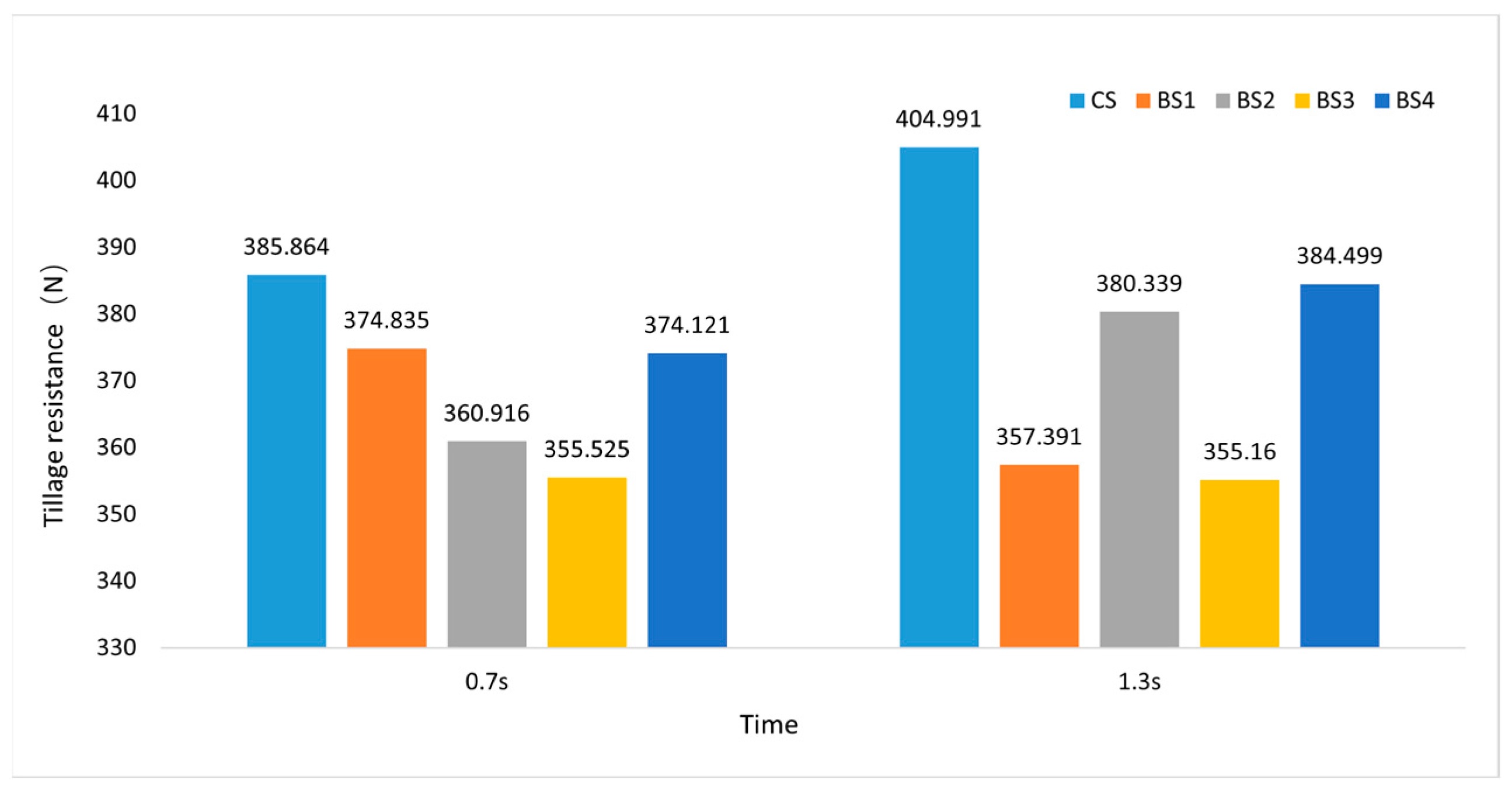
As depicted in Figure 12, the front of the shovel experiences higher forces during stable operation, whether it is a common subsoiling shovel or a bionic subsoiling shovel. Throughout the observation periods, the red area on the bionic shovel’s surface is significantly smaller compared to that on the common shovel, indicating superior resistance reduction performance of the bionic design. Figure 13 illustrates the magnitude of resistance force at two different times, consistent with the visual analysis findings.

Figure 13.
Histogram of tillage resistance to tillage at two times.
For analytical convenience, the average tillage resistance corresponding to each sampling time point in one cycle was calculated, as presented in Table 10. The average total tillage resistance experienced by CS is 391.410 N; the average total tillage resistance experienced by BS1 is 370.610 N, with a drag reduction rate of 5.31%; the average total tillage resistance experienced by BS2 is 355.216 N, with a drag reduction rate of 9.25%; the average total tillage resistance experienced by BS3 is 365.777 N, with a drag reduction rate of 6.55%; the average total tillage resistance experienced by BS4 is 374.704 N, with a drag reduction rate of 2.66%. This indicates that under the same conditions, bionic subsoiling shovels have drag reduction effects, with BS2 having the best drag reduction effect. Combining Figure 11 for analysis, it indicates that the reliability of the experimental analysis is high.
Table 10.
Quantitative analysis of CS and BS tillage performance.
The average tillage resistances experienced by the shovel tip and handle of CS are 247.531 N and 143.879 N, respectively; the average tillage resistances experienced by the shovel tip and handle of BS1 are 237.594 N and 133.594 N, respectively, with drag reduction rates of 4.01% and 7.15%; the average tillage resistances experienced by the shovel tip and handle of BS2 are 219.232 N and 135.985 N, respectively, with drag reduction rates of 11.43% and 5.49%; the average tillage resistances experienced by the tip and handle of BS3 are 233.001 N and 132.769 N, respectively, with drag reduction rates of 5.87% and 7.72%; the average tillage resistances experienced by the tip and handle of BS4 are 219.915 N and 154.789 N, respectively, with drag reduction rates of 8.97% and −7.91%. Except for the increased force on the handle of BS4, the force on all other bionic components is lower than that of CS. The fourth claw toe of the mole cricket’s forefoot is relatively short, and its biological curve characteristics are not as obvious as other claw toes. The curve of the designed BS4 handle is also not as smooth as other shovels, which leads to an increase in its force.
Given that the tip of BS2 demonstrated the most effective resistance reduction, it was combined with the handle of BS3, which had the best resistance reduction effect, to form a bionic subsoiling shovel 5 (BS5). BS5 underwent the same subsoiling simulation, and the average tillage resistance at each sampling time point during stable operation was calculated, as depicted in Table 10.
Although Table 10 illustrates that BS5 has a certain resistance reduction effect, its shovel tip and handle subjected greater forces compared to BS3 and the shovel tip of BS2, and the total resistance it subjected is also the largest among bionic subsoiling shovels.
In summary, although the drag reduction effect of the shovel handles of BS1 and BS3 is slightly better than that of BS2, the tip of BS2 has the best drag reduction effect, and demonstrates the most effective overall resistance reduction. Thus, in terms of resistance reduction, BS2 is preferable, suitable for scenarios with well-conditioned soil and no excessive stones and debris, reducing the loss of the subsoiling shovel while consuming less energy.
3.3. Analysis of Kinetic Energy
The kinetic energy variation of soil particles was obtained, as illustrated in Figure 11d. From Figure 11d, under the action of BS4, the kinetic energy of soil particles is significantly highest; under the action of BS3, the peak kinetic energy of soil particles is greater than that of CS, while under the action of other bionic subsoiling shovels, the kinetic energy of soil particles is significantly lower than that of CS. For the convenience of analysis, the average kinetic energy corresponding to each sampling time point in the stable working stage was calculated, as shown in Table 10. The average soil particle kinetic energies caused by CS, BS1, BS2, BS3, and BS4 are 0.822 J, 0.770 J, 0.735 J, 0.840 J, and 0.931 J, respectively. The energy consumptions of BS1, BS2, BS3, and BS4 are 6.33%, 10.58%, 0.49%, and −14.37% lower than that of CS, respectively. It can be seen that BS1, BS2, and BS3 all have energy reduction effects, and BS1 and BS2 can effectively reduce the energy consumption of deep loosening equipment. Although BS4 exhibits a certain resistance reduction effect, it consumes more energy.
In summary, for energy reduction purposes, BS2 is more effective and better suited for scenarios with more soil stones and high energy consumption, in order to reduce the energy consumption of the subsoiling shovel.
3.4. Analysis of Soil Disturbance
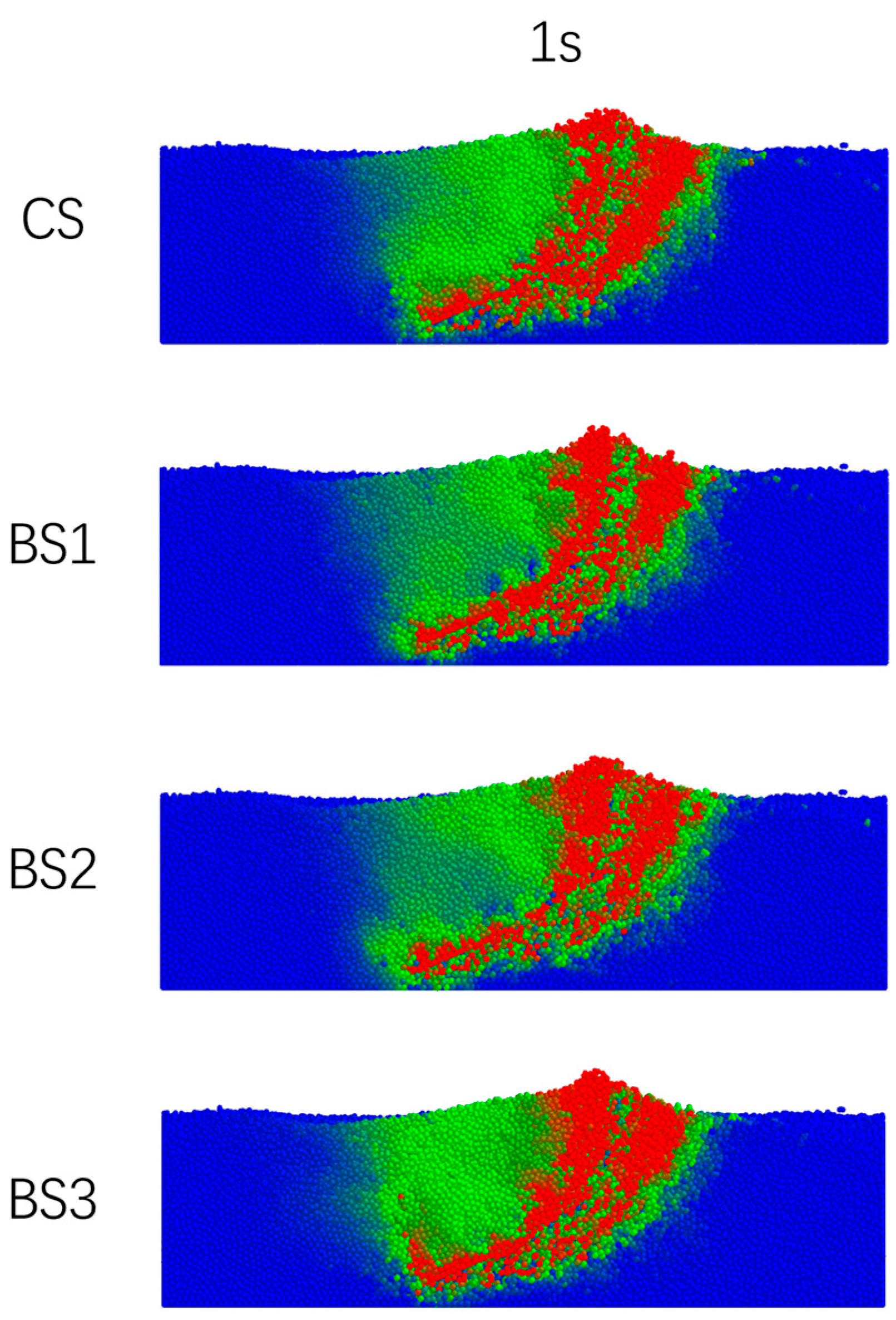
A select velocity cloud diagram of four types of subsoiling shovels disturbing the soil model at 1 s is illustrated in Figure 14. Colors indicate velocity magnitude, with red being the highest, green intermediate, and blue the lowest. In Figure 14, the red area of the soil velocity streamlines for BS1 is smaller than that of CS; BS1 and BS2 exhibit a smaller green area in the soil velocity streamlines compared to CS. Combined with Table 10, it indicates that the reliability of the experimental analysis is high and highlights the energy-saving benefits of BS1 and BS2.

Figure 14.
Velocity cloud diagram.
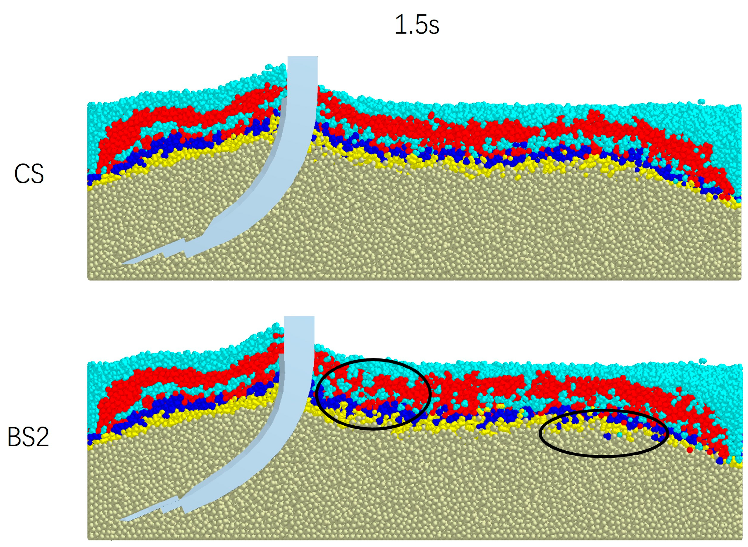
Figure 15 shows the soil model disturbance map at 1.5 s using CS and BS2 with the best drag reduction and energy-saving effects. When the soil particles reach a stable state at the right end of the soil model, it can be seen from the marked part in the figure that under the subsoiling effect of BS2, the particles in the tillage layer are disturbed more severely, and there is a slight exchange of positions between the particles in the tillage layer and the plow layer, indicating that BS2 has better disturbance to the soil.
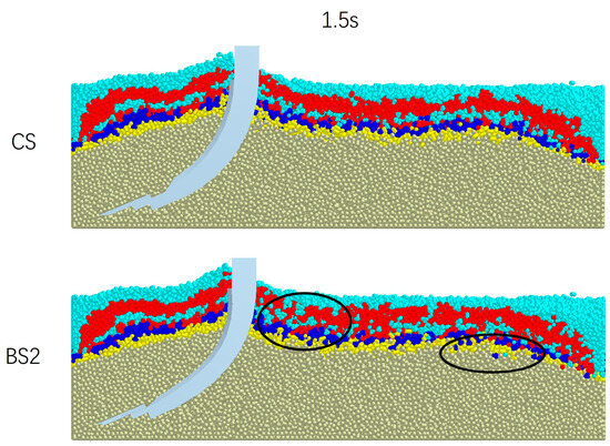
Figure 15.
Visualization of the soil disturbance process.
4. Conclusions
This study took the toes of the mole cricket’s front foot as the biomimetic object, optimized the design of the common subsoiling shovel, adopted the structural biomimetic method to design three biomimetic subsoiling shovels, and calibrated the simulation parameters of red soil in South China, with optimal parameters determined through steepest climbing tests and Design-Expert.13 and using the soil accumulation angle as the response value. This study also conducted discrete element modeling and numerical simulation of soil and subsoiling shovels. When using EDEM 2020 for discrete element soil modeling of red soil, a separate plow pan was made and a soil-modeling method of preset force compression was adopted, which is more in line with the actual structure of red soil.
The subsoiling effect was analyzed using metrics such as average tillage resistance, kinetic energy of soil particles, soil disturbance, and soil particle velocity. The results demonstrated that compared with the common subsoiling shovel, the bionic subsoiling shovel 1 experienced a 5.31% reduction in tillage force, with a 4.01% reduction in tillage force at the shovel tip, a 7.15% reduction in tillage force at the shovel handle, and a 6.33% reduction in energy consumption. The biomimetic subsoiling shovel 2 experienced a 9.25% reduction in tillage force, with an 11.43% reduction in tillage force at the tip, a 5.49% reduction in tillage force at the handle, and a 10.58% reduction in energy consumption. The biomimetic subsoiling shovel 3 experienced a 6.55% reduction in tillage force, with a 5.87% reduction in tillage force at the tip, a 7.72% reduction in tillage force at the handle, and a 0.49% reduction in energy consumption. Further verification has shown that compared to common subsoiling shovels, these three bionic subsoiling shovels have better resistance reduction and energy reduction effects. After comprehensive consideration, it is believed that the bionic subsoiling shovel 2 is the best choice and should continue to be used for research in the future. This conclusion means that in future work, we should conduct more research on bionic designs to reduce tillage resistance.
Author Contributions
Conceptualization, methodology, data curation, writing—review and editing, validation, and formal analysis, L.Z.; conceptualization, methodology, software, data curation, and writing-original draft, X.W.; software, data curation, H.W. and Y.C.; supervision, project administration, and funding acquisition, J.C. All authors have read and agreed to the published version of the manuscript.
Funding
This work was supported by the National Natural Science Foundation of China (Grant No. 32372005).
Institutional Review Board Statement
Not applicable.
Data Availability Statement
All data are presented in this article in the form of figures and tables.
Acknowledgments
We thank editors and anonymous reviewers for providing useful suggestions for improving the quality of papers.
Conflicts of Interest
The authors declare no conflicts of interest.
References
- Xu, X.D.; Jing, P.Y.; Yao, Q.; Chen, W.H.; Meng, H.W.; Li, X.; Qi, J.T.; Peng, H.J. Parameter Optimization and Test for the Pulse-Type Gas Explosion Subsoiler. Agriculture 2024, 14, 1417. [Google Scholar] [CrossRef]
- Yue, L.K.; Wang, Y.; Wang, L.; Yao, S.H.; Cong, C.; Ren, L.D.; Zhang, B. Impacts of soil compaction and historical soybean variety growth on soil macropore structure. Soil Tillage Res. 2021, 214, 105166. [Google Scholar] [CrossRef]
- Schneider, F.; Don, A.; Hennings, I.; Schmittmann, O.; Seidel, S.J. The effect of deep tillage on crop yield—What do we really know? Soil Tillage Res. 2017, 174, 193–204. [Google Scholar] [CrossRef]
- Wang, Y.M.; Li, N.; Ma, Y.H.; Tong, J.; Pfleging, W.; Sun, J. Field experiments evaluating a biomimetic shark-inspired (BioS) subsoiler for tillage resistance reduction. Soil Tillage Res. 2020, 196, 104432. [Google Scholar] [CrossRef]
- Zhou, D.Y.; Hou, P.F.; Xin, Y.L.; Wu, B.G.; Tong, J.; Yu, H.Y.; Qi, J.T.; Zhang, J.S.; Zhang, Q. Resistance and Consumption Reduction Mechanism of Bionic Vibration and Verification of Field Subsoiling Experiment. Appl. Sci. 2021, 11, 10480. [Google Scholar] [CrossRef]
- Long, Z.J.; Wang, Y.F.; Sun, B.R.; Tang, X.Y.; Jin, K.M. Impact of mechanical compaction on crop growth and sustainable agriculture. Front. Agr. Sci. Eng 2024, 11, 243–252. [Google Scholar] [CrossRef]
- Qiu, L.K. Study on the Response of Crop Species and Varieties to Mollisol Compaction. Ph.D. Thesis, Chinese Academy of Agricultural Sciences, Beijing, China, 2019. [Google Scholar]
- Jéssica, F.S.; Miguel, J.R.; Dörthe, H.; Fernanda, M.R.; Frank, E.A. Subsoiling and mechanical hole-drilling tillage effects on soil physical properties and initial growth of eucalyptus after eucalyptus on steeplands. Soil Tillage Res. 2020, 207, 104860. [Google Scholar] [CrossRef]
- Wang, H.B.; Bai, W.B.; Han, W.; Song, J.Q.; Lv, G.H. Effect of subsoiling on soil properties and winter wheat grain yield. Soil Use Manag. 2019, 35, 643–652. [Google Scholar] [CrossRef]
- Zhang, C.X.; Guo, J.; Ma, F.Y.; Yu, F.X.; Hou, Z.H.; Wang, L.H.; Fang, J.Y.; Tang, F.Y. Effects of vertical rotary subsoiling with plastic mulching on soil water availability and potato yield on a semiarid Loess plateau, China. Soil Tillage Res. 2020, 199, 104591. [Google Scholar] [CrossRef]
- Zhang, L.; Zhai, Y.B.; Chen, J.N.; Zhang, Z.E.; Huang, S.Z. Optimization design and performance study of a subsoiler underlying the tea garden subsoiling mechanism based on bionics and EDEM. Soil Tillage Res. 2022, 220, 105375. [Google Scholar] [CrossRef]
- Lu, Y. Design and Experimental Study of Bionic Energy Storage-Profiling Deep Loosening Device. Ph.D. Thesis, Jilin University, Jilin, China, 2023. [Google Scholar]
- Zhang, X.R.; Zeng, W.Q.; Liu, J.X.; Wu, P.; Dong, X.H.; Hu, H.N. Design and experiment of inclined handle folded wing deep loosening shovel for brick red soil based on discrete element method. Trans. Chin. Soc. Agric. Mach 2022, 53, 40–49. [Google Scholar]
- Song, W.; Jiang, X.H.; Li, L.K.; Ren, L.L.; Tong, J. Increasing the width of disturbance of plough pan with bionic inspired subsoilers. Soil Tillage Res. 2022, 220, 105356. [Google Scholar] [CrossRef]
- Sun, J.F.; Chen, H.M.; Wang, Z.M.; Ou, Z.; Yang, Z.; Liu, Z.; Duan, J.L. Study on plowing performance of EDEM low-resistance animal bionic device based on red soil. Soil Tillage Res. 2020, 196, 104336. [Google Scholar] [CrossRef]
- Foldager, F.F.; Munkholm, L.J.; Balling, O.; Serban, R.; Negrut, D.; Heck, R.J.; Green, O. Modeling soil aggregate fracture using the discrete element method. Soil Tillage Res. 2022, 218, 105295. [Google Scholar] [CrossRef]
- Goodwin, C.G.; Medioli, M.A.; Sher, W.; Vlacic, B.L.; Welsh, J.S. Emulation-Based Virtual Laboratories: A Low-Cost Alternative to Physical Experiments in Control Engineering Education. IEEE Trans. Educ. 2011, 54, 48–55. [Google Scholar] [CrossRef]
- Zhang, Y. The Research on Coupling Characteristics, Kinematics Modeling and Bionic Application of Mole Criket (Gryllotalpa orientalis). Ph.D. Thesis, Jilin University, Jilin, China, 2011. [Google Scholar]
- Zeng, Z.W.; Ma, X.; Chen, Y.; Qi, L. Modelling residue incorporation of selected chisel ploughing tools using the discrete element method (DEM). Soil Tillage Res. 2020, 197, 104505. [Google Scholar] [CrossRef]
- Saunders, C.; Ucgul, M.; Godwin, J.R. Discrete element method (DEM) simulation to improve performance of a mouldboard skimmer. Soil Tillage Res. 2021, 205, 104764. [Google Scholar] [CrossRef]
- Hang, C.G.; Gao, X.J.; Yuan, M.C.; Huang, Y.X.; Zhu, R.X. Discrete element simulations and experiments of soil disturbance as affected by the tine spacing of subsoiler. Biosyst. Eng. 2018, 168, 73–82. [Google Scholar] [CrossRef]
- Fang, H.M.; Ji, C.Y.; Ahmed, A.T.; Zhang, Q.Y.; Guo, J. Simulation analysis of straw movement in straw-soil-rotary blade system. Trans. Chin. Soc. Agric. Mach 2016, 47, 60–67. [Google Scholar] [CrossRef]
- Chen, Y.; Munkholm, J.L.; Nyord, T. A discrete element model for soil–sweep interaction in three different soils. Soil Tillage Res. 2013, 126, 34–41. [Google Scholar] [CrossRef]
- Tamás, K.; Jóri, J.I.; Mouazen, M.A. Modelling soil–sweep interaction with discrete element method. Soil Tillage Res. 2013, 134, 223–231. [Google Scholar] [CrossRef]
- Sun, J.Y.; Wang, Y.M.; Ma, Y.H.; Tong, J.; Zhang, Z.J. DEM simulation of bionic subsoilers (tillage depth 40 cm) with drag reduction and lower soil disturbance characteristics. Adv. Eng. Softw. 2018, 119, 30–37. [Google Scholar] [CrossRef]
- Wang, Y.; Zhang, D.; Yang, L.; Cui, T.; Jing, H.; Zhong, X. Modeling the interaction of soil and a vibrating subsoiler using the discrete element method. Comput. Electron. Agric. 2020, 174, 105518. [Google Scholar] [CrossRef]
- Zhang, Y. Biology Coupling Characteristics on Soil-Engaging Components of Mole Crickets. Master’s Thesis, Jilin University, Jilin, China, 2008. [Google Scholar]
- Zhang, S.B. Desing and Analysis of a Biomimetic Excavator Bucket Bioinspired by the Characteristics of Mole Cricket Claw. Master’s Thesis, Tianjin University of Science and Technology, Tianjin, China, 2015. [Google Scholar]
- Gao, H. Characteristic, Function, Mechanics and Bionic Analysis of Oriental Mole Cricket (Gryllotalpa orientalis Burmeister). Ph.D. Thesis, Jilin University, Jilin, China, 2009. [Google Scholar]
- Zhu, H.; Wang, D.W.; He, X.N.; Shang, S.Q.; Zhao, Z.; Wang, H.Q.; Tan, Y.; Shi, Y.X. Study on Plant Crushing and Soil Throwing Performance of Bionic Rotary Blades in Cyperus esculentus Harvesting. Mach 2022, 10, 562. [Google Scholar] [CrossRef]
- Wang, P.F. Study on Resistance Reduction Mechanism Based on Mole Cricket Claw Toe Structure. Master’s Thesis, Tianjin University of Science and Technology, Tianjin, China, 2020. [Google Scholar] [CrossRef]
- Xing, J.J.; Zhang, R.; Wu, P.; Zhang, X.R.; Dong, X.H.; Chen, Y.; Ru, S.F. Parameter Calibration of Discrete Element Simulation Model for Red Soil Particles in Hainan Hot Zone. Trans. Chin. Soc. Agric. Eng. 2020, 36, 158–166. [Google Scholar]
- Zhai, Y.B. Design and Experiment of a Bionic Subsoiling Mechanism for Hilly and Mountainous Farmland Based on DEM. Master’s Thesis, Zhejiang Sci-Tech University, Hangzhou, China, 2023. [Google Scholar] [CrossRef]
- Wang, Y. Simulation Analysis of Structure and Effect of the Subsoiler Based on DEM. Master’s Thesis, Jilin Agricultural University, Changchun, China, 2014. [Google Scholar]


Disclaimer/Publisher’s Note: The statements, opinions and data contained in all publications are solely those of the individual author(s) and contributor(s) and not of MDPI and/or the editor(s). MDPI and/or the editor(s) disclaim responsibility for any injury to people or property resulting from any ideas, methods, instructions or products referred to in the content. |
© 2024 by the authors. Licensee MDPI, Basel, Switzerland. This article is an open access article distributed under the terms and conditions of the Creative Commons Attribution (CC BY) license (https://creativecommons.org/licenses/by/4.0/).