The More the Better? Reconsidering the Welfare Effect of Crop Insurance Premium Subsidy

Abstract

China has invested substantial financial subsidies to promote the development of crop insurance; however, the insurance demand among farmers remains notably low, resulting in significant welfare loss. Based on a field survey conducted in 2021 in seven major grain-producing counties in Jiangsu Province, this study analyses the relationship between premium subsidy rates and the welfare effects of subsidies through theoretical model derivation and explores the impact of farmer heterogeneity on the results. This study innovatively introduces a power law distribution model to elucidate the distributional characteristics of farmers’ crop insurance demand, demonstrates the significant limitations of the linear demand model in welfare research, and effectively analyzes the welfare effects of China’s current crop insurance premium subsidy policy. The results indicate that: (1) the actual crop insurance demand of farmers aligns more closely with a power law distribution, and its long-tailed characteristics refute the assumption of linear distribution; (2) there exists an inverted “U”-shaped relationship between the subsidy ratio and the welfare effect, and an excessively high subsidy ratio produces substantial unnecessary losses; (3) variations in welfare effects exist among farmers in different regions, risk attitudes, and cultivation scales, but the range of differences between groups is limited.

1. Introduction

Crop insurance is an important mechanism in China to help stabilize food production and protect farmers’ income. However, the recent increase in severe natural disasters has posed significant challenges to the risk-mitigation function of crop insurance and jeopardized the stability of agricultural earnings [1]. The current challenge in crop insurance development lies in enhancing the efficacy of insurance subsidy policies to mitigate the impact of extreme weather events on agricultural operations, which has been the focus of attention of researchers and scholars in recent years [2].

Crop insurance has played a crucial role in the modernization of Chinese agriculture. Compared to other countries with more established crop insurance development, such as the United States, Canada, and Japan, China’s crop insurance subsidy policy system was initiated relatively recently, with the pilot promotion of policy crop insurance beginning only in 2007, and the subsidized varieties limited to five crops. Nevertheless, over the past decade, the Chinese government has continuously improved and standardized the subsidy policy, and the scale of premiums and the depth and breadth of insurance have maintained a substantial growth rate. As of 2020, China’s total crop insurance premium income reached CNY 81.5 billion (the exchange rate between the USD and the CNY on 22 October 2024 is: USD 1 = CNY 7.12), establishing it as the world’s largest agricultural insurance market (data from China Banking and Insurance Regulatory Commission). Currently, the total proportion of premium subsidies for crop insurance by Chinese governments at all levels has stabilized at approximately 80%, effectively contributing to the increased demand for crop insurance, providing 164 million farmers with CNY 4.98 trillion of risk protection in 2023, and significantly reducing the impact of natural disasters on farmers’ agricultural production (data from a press release by the State Council of China).

However, since the outbreak of COVID-19, China’s economic growth has slowed, and the pressure on fiscal revenues and expenditures at all levels has increased sharply under the dual impact of an economic downturn and tax and fee reductions [3]. Nevertheless, studies have shown that increased premium subsidies have had many positive effects on the development of agricultural insurance in China, such as increasing the insurance penetration rate, solving moral hazard, and stabilizing food security [4,5,6,7]. However, the expansion of subsidies has also brought a number of negative effects, in particular the increasing fiscal pressure caused by subsidies, which may limit the Chinese government’s ability to allocate funds, and then lead to risks such as misallocation of resources and increased administrative costs [8,9,10,11]. In addition, China’s subsidy policy has been shown to increase farmers’ income, but also to exacerbate the destruction of the agricultural environment and hinder the green development of agriculture [2,12]. Meanwhile, the actual demand for crop insurance in China remains low due to factors such as farmers’ limited insurance knowledge and unregulated insurance experience [13]. Therefore, an effective evaluation of China’s crop insurance premium subsidy policy and the measurement of the welfare effects generated by the premium subsidy are conducive to the government’s rational planning of financial resources and the optimization of social welfare.

Existing studies have analyzed the welfare effects of crop insurance premium subsidy policies in different ways [14,15]. The study by Ye et al. [16] found that farm households prefer highly subsidized insurance products, and the government can take advantage of this to increase the welfare of the insured by introducing new insurance products while keeping the subsidy level constant. The study by Ramirez and Carpio [17] shows that the effectiveness of subsidies varies widely across groups, with more subsidies going to farmers who already have a lower willingness to pay (WTP). The study by Alizamir et al. [18] shows that increasing the welfare of farm households through premium subsidy policies leads to a higher loss of fiscal resources.

However, most of these studies focus on analyzing optimal premium subsidy policies under different insurance and subsidy models [19,20], ignoring the impact of the accuracy and validity of welfare assessment models on the veracity of welfare findings [21,22,23]. Many studies have been analyzed without sufficiently discussing the assumptions and limitations used in the demand models, even directly assuming that crop insurance demand is linearly distributed [21,24,25,26]. In general, aggregate demand needs to satisfy the assumption of the existence of ‘representative consumers’ for a sexual demand distribution to emerge [27,28]. However, many studies have pointed out the limitations of this strong assumption [29,30,31], especially considering the effect of heterogeneity of farm households on individual demand curves [32,33], and the fact that differences in individual marginal demand inevitably lead to a heterogeneous distribution of aggregate demand curves [28]. In fact, many research data also show that in reality farmers’ crop insurance demand shows a nonlinear distribution [34,35,36]. Therefore, simply treating all farmers as a homogeneous consumer group and linearizing the insurance demand model clearly violates the premise assumptions of the linear demand model. If the wrong demand model is used to measure the subsidy welfare effect, it will undoubtedly lead to bias or even error in the final results. Based on this, this study aims to explore the actual demand status of farmers for crop insurance so that a demand model can be constructed that can truly reflect the distribution of demand in the crop insurance market. At the same time, the study also attempts to clarify the complex relationship between the premium subsidy rate of crop insurance and the welfare effect of the subsidy based on a reasonable insurance demand model, so as to delineate a reasonable interval for the premium subsidy rate. The study analyses the welfare effects of changes in crop insurance premium subsidy rates by constructing two hypothetical models with linear and non-linear demand distributions, thus demonstrating how differences in demand models affect the results of the subsidy welfare effect analysis. To this end, a field survey of farmer demand for new wheat insurance was conducted in seven major grain-producing counties in Jiangsu Province in 2021 to fulfil the research objectives of this study.

Our study makes the following contributions: First, compared to previous crop insurance studies based on linear demand distribution assumptions [21,24,25,26], this paper innovatively introduces the power law distribution model into the analysis of crop insurance demand distribution, which provides a more consistent analytical model of the real demand for crop insurance. At the same time, the study demonstrates the limitations of this linear demand model assumption in researching the impact assessment of crop insurance premium subsidy policies from the theoretical level. Finally, in contrast to the results of the welfare effect analyses of premium subsidies in previous studies [14,15,16,17,18], we find that the relationship between the proportion of crop insurance premium subsidies and the welfare effects of the subsidies is not a simple upward or downward relationship, but an inverted U-shaped relationship in which the proportion of crop insurance premium subsidies first increases and then decreases. This suggests that excessive increases in premium subsidies not only fail to effectively improve farmers’ welfare, but also lead to a large loss of subsidies. In addition, the study identifies an appropriate range of premium subsidy ratios to help policymakers improve the efficiency of crop insurance subsidy policies in the future.

The sections of this study are structured as follows: Section 2 outlines the materials and methods, which mainly reviews the related literature, presents the theoretical model of this study, and the sources and characteristics of the research data; Section 3 shows the results, which presents the empirical results of this study and the related robustness tests and heterogeneity analyses; Section 4 is the discussion; and Section 5 is the conclusion.

2. Materials and Methods

2.1. Theoretical Analysis

This section constructs two hypothetical models of demand distribution, linear and non-linear, based on the market equilibrium model in welfare economics [37,38,39,40]. The study analyses the impact of changes in the proportion of premium subsidies on the welfare of farm households, welfare losses, and further elucidates the welfare effects of subsidies. The study quantifies the welfare effect of premium subsidies by calculating the increase in farmers’ welfare subsequent to the increase in subsidies, minus the increase in welfare losses. Given China’s policy requirement that all farmland must be insured when a farmer opts for insurance, the model assumes that a farmer’s insured area is equivalent to his or her cultivated area. Since the price of crop insurance in China is established by the government with the approval of the insurance company after it is proposed by the insurance company, its price does not fluctuate with market changes as other commodities do; thus, the insurance supply line is horizontal. It is noteworthy that the slope of the supply line does not affect the results of the study, as demonstrated by the outcomes of subsequent studies.

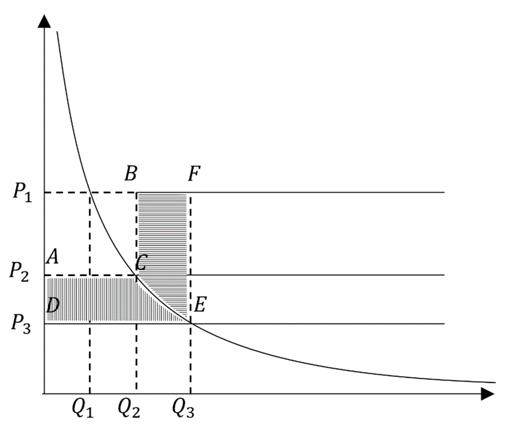
2.1.1. Welfare Analysis Under a Linear but Irrational Demand Model

Initially, this study analyses the impact of the premium subsidy rate on welfare under a linear demand model. In the absence of government subsidy, the price of insurance is higher, at which point the supply curve is assumed to be represented by BI in Figure 1. The intervention of the government subsidy will result in farmers paying less for crop insurance, thus increasing insurance coverage.

In accordance with the linear demand model, it is postulated that the demand curve exhibits a linear relationship with a negative slope, as represented by line AH in Figure 1. The demand function is expressed as:

$$Q=a+bP$$

(1)

In Equation (1), $P$ denotes the premium, $Q$ represents the total area insured at premium $P$, $a$ signifies the intercept term between the demand line and the Y-axis, and $b$ represents the coefficient of the premium $P$. In accordance with the law of demand, we assume that $a>0$ and $b<0$. Let us consider that the market price of insurance without subsidy is $P_1$ and the supply line is BI. The minimum enrollment rate serves as the foundation for the insurer to ensure the operational viability of crop insurance [41]. The demand $Q_2$, which is predicated on the minimum insurance coverage, represents the corresponding insurance demand. Given that the demand for insurance $Q_1$ is substantially lower than the minimum insurance rate, the crop insurance market cannot be established at this juncture. Consequently, government intervention is necessary to provide a subsidy to reduce the premium to $P_2$, resulting in the supply line shifting downward to EF. At this point, the crop insurance market is initially established, and assuming further government subsidization of the premium, the premium level $P_2$ is reduced to $P_3$, with the difference between $P_2$ and $P_3$ being $∆P=P_2-P_3$. When farmers purchase crop insurance at the price level of $P_3$, the additional government subsidy is represented by the shaded area in Figure 1 (DIHE and FEHG). The resulting additional consumer surplus $∆{CS}_1$ is depicted by the FEHG region:

$${∆CS}_1={\displaystyle \frac{(Q_2+Q_3)∆P}{2}}$$

(2)

The additional deadweight loss is depicted by the DEHI region:

$${∆DWL}_1={\displaystyle \frac{\left({2P}_1-P_2-P_3\right)\left(Q_3-Q_2\right)}{2}}$$

(3)

Drawing on Zhu et al.’s [42] study, this study quantifies the welfare effect of additional subsidies by utilizing the net welfare growth of additional farmer benefits minus the deadweight loss of additional subsidies. The formula is as follows:

$$Welafre{effectchange}_1=∆C{S}_1-∆DW{L}_2$$

(4)

Furthermore, this study illustrates the trend of the welfare effect of the additional subsidy more comprehensively by comparing the additional farmers’ welfare with the additional deadweight loss, yielding a ratio of $g_1$. The magnitude of $g_1$ is directly proportional to the impact of the additional subsidy on the level of farmers’ welfare. The specific methodology for the derivation of the linear demand model is as follows:

$$\begin{gathered} g_1={\displaystyle \frac{{∆CS}_1}{{∆DWL}_1}} \\ ={\displaystyle \frac{\left(Q_3+Q_2\right)∆P}{\left({2P}_1-P_2-P_3\right)\left(Q_3-Q_2\right)}} \\ ={\displaystyle \frac{\left(a+b{P}_3+a+b{P}_2\right)∆P}{\left({2P}_1-P_2-P_3\right)\left(a+b{P}_3-a-b{P}_2\right)}} \\ ={\displaystyle \frac{2a-b(∆P-2P_2)}{-2b{P}_1-b(∆P-2P_2)}} \end{gathered}$$

(5)

The ratio $g_1$ is crucial for evaluating whether the additional deadweight loss will exceed the additional gain to the farmer. In $g_1$, the primary distinction between the numerator and denominator lies in the initial term. As the demand for crop insurance $Q_1$ > 0, $g_1$ is consistently greater than 1. This indicates that under the linear demand assumption, the additional deadweight loss does not surpass the welfare gains to the farmer. Consequently, within the linear demand model, the government subsidy will only yield a positive welfare effect. If the welfare gains to farmers from subsidies exceeding the welfare loss is considered as the effective subsidy rate, then a higher subsidy rate corresponds to a greater welfare effect and increased subsidy effectiveness. The sensitivity of welfare gains to changes in subsidies can be further characterized using the first-order derivative of the subsidy rate $g_1$ with respect to premiums. In the simplified $g_1$, only $P_2$ is unknown, and the derivative with respect to $P_2$ can be derived and simplified as:

$$\begin{gathered} {\displaystyle \frac{d{g}_1}{d{P}_2}}={\displaystyle \frac{{\left(2a+2b{P}_2-b∆P\right)}^{\prime }\left(2b{P}_2-2b{P}_1-b∆P\right)}{({2b{P}_2-2b{P}_1-b∆P)}^2}} \\ -{\displaystyle \frac{{\left(2a+2b{P}_2-b∆P\right)\left(2b{P}_2-2b{P}_1-b∆P\right)}^{\prime }}{({2b{P}_2-2b{P}_1-b∆P)}^2}} \\ ={\displaystyle \frac{-4b(a+b{P}_1)}{(-{2b{P}_1+2b{P}_2-b∆P)}^2}} \end{gathered}$$

(6)

According to Equation (6), the denominator $a$ is consistently greater than 0, $b$ in the numerator is negative, and $a+b{P}_1=Q_1$ is also greater than 0; consequently, the ratio $g_1$ increases monotonically with the increase in premiums. This implies that the ratio $g_1$ decreases as the premium subsidy increases. This observation leads to the conclusion that the stimulating effect of premium subsidies on the growth of welfare effects diminishes with increasing subsidies. Therefore, we propose the following hypothesis:

Hypothesis 1:

Given the assumption of linear demand for crop insurance, the magnitude of the welfare effect of the subsidy is positively correlated with the premium subsidy level; however, the subsidy’s stimulative effect on welfare exhibits diminishing returns.

2.1.2. Welfare Analysis Under Non-Linear Real Model

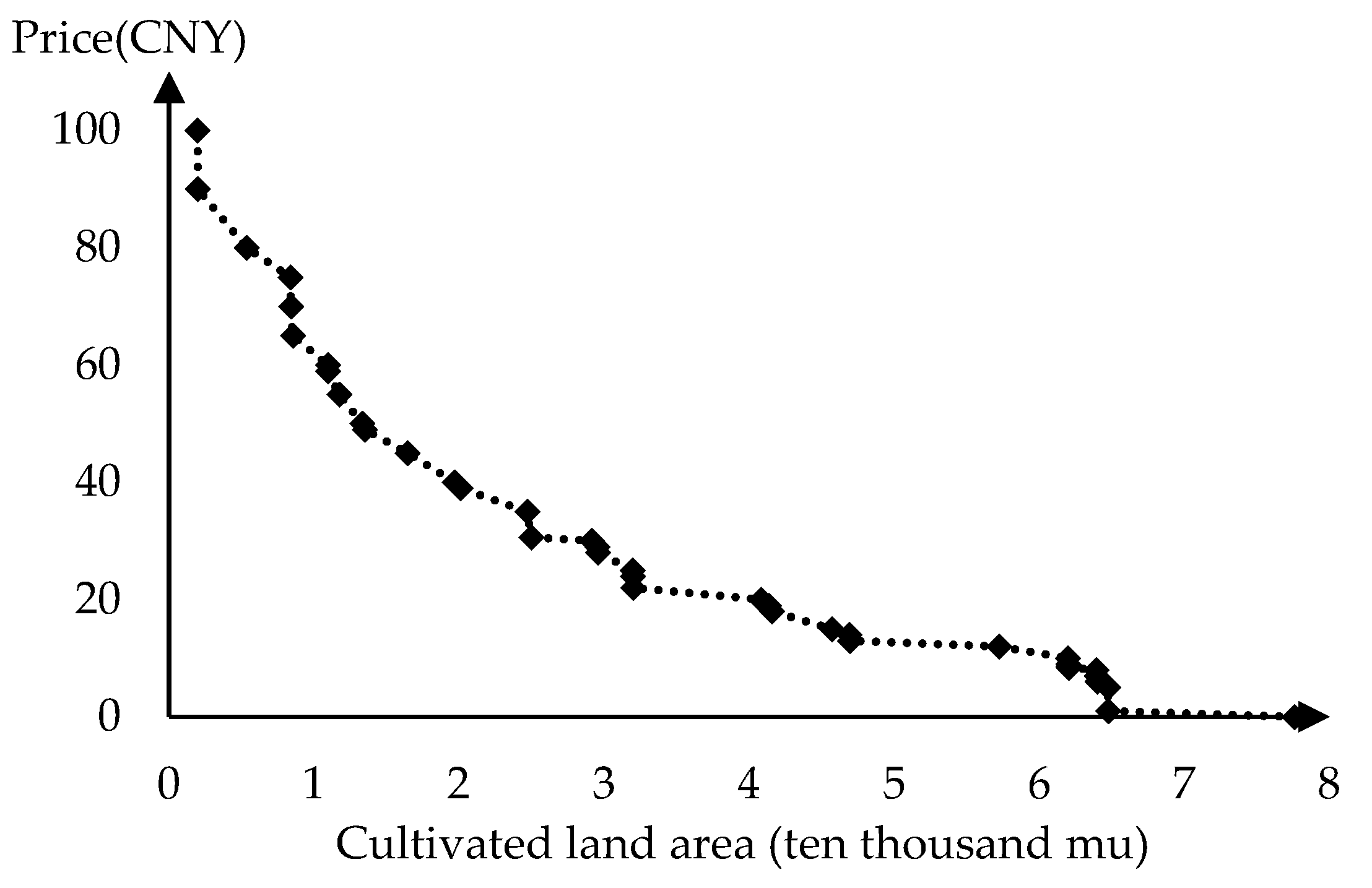
This section draws upon extant literature that has modified the curvature of the demand line in market equilibrium models to analyze welfare changes and constructs a model of insurance demand that utilizes a power law distribution as an assumption to examine the welfare effects of subsidies [39,40]. When crop insurance demand conforms to a power law function, the demand curve can be represented by the demand function illustrated in Figure 2.

As is characteristic of many power law distributions observed in education, wealth, and commodity consumption [43,44], the majority of farmers are unable to afford high premiums and only purchase insurance when prices are low, which elucidates the unsustainability of the commercial crop insurance model [45]. Consequently, this study establishes a power law distribution model to quantify the welfare effect of crop insurance subsidies:

$$Q=a{P}^b$$

(7)

where $P$ denotes the premium and $Q$ denotes the insured acreage at that premium level. Both price and demand are inherently non-negative, which implies that $a$ > 0 and $b$ < 0. Although the traditional power law function corresponds to $a=1$, the insurance market may introduce variables that result in $a\ne 1$. However, the value of $a$ is not important to the results of the study; it only affects the vertical position of the demand curve. When the premium price is $P_1$, the demand $Q_1$ cannot satisfy the minimum insured demand $Q_2$. It is assumed that after a certain level of subsidy, the increased demand satisfies the minimum insured rate, at which point the premium is $P_2$ and the demand is $Q_2$. Assume that a further increase in the subsidy will cause the premium $P_2$ to decrease by $∆P$ to $P_3$, at which point the demand reaches $Q_3$. As illustrated in Figure 2, the additional benefit to the farmer ${∆CS}_2$ is represented by the area of the ACED:

$$\begin{gathered} {∆CS}_2=Q_2∆P+{\int }_{P_3}^{P_2}\left(a{P}^b-Q_2\right)dP \\ ={\displaystyle \frac{a{P_2}^{1+b}-a{P_3}^{1+b}}{1+b}} \end{gathered}$$

(8)

The additional deadweight loss ${∆DWL}_2$ is the area of BCFE:

$$\begin{gathered} {∆DWL}_2=\left(Q_3-Q_2\right)\left(P_1-P_3\right)-{\int }_{P_3}^{P_2}\left(a{P}^b-Q_2\right)dP \\ =\left(a{P_3}^b-a{P_2}^b\right)\left(P_1-P_3\right)-{\displaystyle \frac{a{P_2}^{1+b}-a{P_3}^{1+b}}{1+b}}+a{P_2}^b∆P \end{gathered}$$

(9)

The differential between a farmer’s additional welfare and the additional deadweight loss can be simplified as:

$$\begin{gathered} {Welfare{effectchange}_2=∆DWL}_2-{∆CS}_2 \\ =\left(a{P_3}^b-a{P_2}^b\right)\left(P_1-P_3\right)-{\displaystyle \frac{a{P_2}^{1+b}-a{\left(P_3\right)}^{1+b}}{1+b}}+a{P_2}^b∆P \\ -{\displaystyle \frac{a{P_2}^{1+b}-a{\left(P_2-∆P\right)}^{1+b}}{1+b}} \\ =\left({\displaystyle \frac{1-b}{1+b}}a{P_3}^{1+b}+a{P_3}^b{P}_1\right)-\left({\displaystyle \frac{1-b}{1+b}}a{P_2}^{1+b}+a{P_2}^b{P}_1\right) \end{gathered}$$

(10)

From the simplified Equation (10), the functional form of the two parts before and after is identical; therefore, a new functional form can be established as:

$$f\left(x\right)={\displaystyle \frac{1-b}{1+b}}a{x}^{1+b}+a{P}_1{x}^b$$

(11)

where $b\ne -1$. To determine whether the difference between the new farmers’ welfare and the new deadweight loss is positive or negative, the monotonicity of $f(x)$ must be specified. We let $x>0$ and then make the derivative of $f(x)$ and make $f^{\prime }(x)$ equal to 0. We then obtain the critical point $x^{\ast }={\displaystyle \frac{-b{P}_1}{1-b}}$. We further find the second-order derivative of the function $f(x)$ and bring in the critical point obtained from the first-order derivative. We could obtain:

$$f^{″}(x)=-a\left(b-1\right)b{x}^{b-2}·\left(x-P_1\right)$$

(12)

$$f^{″}\left({\displaystyle \frac{-b{P}_1}{1-b}}\right)=ab\left(1-b\right)b({{\displaystyle \frac{-b{P}_1}{1-b}})}^{b-2}({\displaystyle \frac{-b{P}_1}{1-b}}-P_1)$$

(13)

$$=a(1-b){({\displaystyle \frac{1-b}{-b{P}_1}})}^{1-b}$$

According to Equation (13), the second-order derivative of the function $f\left(x\right)$ is constantly greater than 0 in the limit of $b>-1$. Consequently, it is a monotonically increasing function when $x>{\displaystyle \frac{-b{P}_1}{1-b}}$ and a monotonically decreasing function when $x<{\displaystyle \frac{-b{P}_1}{1-b}}$. In accordance with the parameters of this study, the ratio $g$, obtained by dividing the new farmers’ welfare by the new deadweight loss, serves as an indicator of the pulling effect of the welfare effect of the crop insurance premium subsidy. As per the aforementioned equation, the expression for $g$ is:

$$g={\displaystyle \frac{\frac{a{P_2}^{1+b}-a{P_3}^{1+b}}{1+b}}{\left(a{P_3}^b-a{P_2}^b\right)\left(P_1-P_3\right)-\frac{a{P_2}^{1+b}-a{P_3}^{1+b}}{1+b}+a{P_2}^b∆P}}$$

$$={\displaystyle \frac{{P_2}^{1+b}-{P_3}^{1+b}}{\left(1+b\right)\left({P_3}^b-{P_2}^b\right)\left(P_1-P_3\right)-{P_2}^{1+b}+{P_3}^{1+b}+{{(1+b)P}_2}^b∆P}}$$

(14)

Further finding the derivative of $P_2$ with respect to $g$, we get:

$${\displaystyle \frac{dg}{d{P}_2}}=-{\displaystyle \frac{(b+1)P_1({P_3}^{2b}{P}_2{P}_3+{P_2}^{2b}{P}_2{P}_3+{P_2}^b{P_3}^b\left(b{∆P}^2-2P_2{P}_3\right))}{P_2{P}_3{({P_3}^b\left(b{P}_2+\left(-b-1\right)P_1-b∆P\right)+{P_2}^b\left(\left(b+1\right)P_1-b{P}_2\right))}^2}}$$

(15)

where ${P_2}^b{P_3}^{b}b{∆P}^2$ is negative, $2{P_2}^{b+1}{P_3}^{b+1}$ is positive, and the formula $({P_3}^{2b}{P}_2{P}_3+{P_2}^{2b}{P}_2{P}_3+{P_2}^b{P_3}^b(b{∆P}^2-2P_2{P}_3)$) is positive. Based on the aforementioned derivative, the first-order derivative of $g$ is negative when $-1<b<0$, and the ratio $g$ monotonically decreases with the increase in $P_2$. When $b<-1$, the first-order derivative is positive, and the ratio $g$ monotonically increases with the increase in $P_2$. Based on the estimates of $b$ obtained from the empirical analysis in the main text, we conclude that, under the power-law model, ratio $g$ decreases monotonically with an increase in the subsidy ratio and a decrease in the price.

Therefore, in the power-law demand model, a subsidy policy that aims to maximize the welfare effect of subsidies deviates from a subsidy policy that aims to maximize farmers’ welfare. When a critical subsidy ratio is reached, the government must cease increasing premium subsidies to prevent the misallocation of funds. Consequently, the hypothesis is that:

Hypothesis 2:

Under the assumption of a power law function of crop insurance demand, increased premium subsidies enhance farmers’ welfare. However, the welfare effect of subsidies exhibits an inverted ‘U’ pattern, initially increasing and subsequently decreasing.

2.2. Data Source

This study was conducted in December 2021 in seven counties of Yancheng City, Suqian City, and Huai’an City in Jiangsu Province, and a map of the study area is shown in Supplementary Figure S1. All three regions will implement a new crop insurance program by 2022, and the majority of local farmers grow wheat and purchase crop insurance. The research covered six main areas: farmers’ household characteristics, agricultural production information, agricultural risk perceptions and experiences with crop insurance, household income and expenditures, personal risk preferences, and WTP for the new crop insurance. Compared with the previous wheat insurance purchased by farmers, the maximum payout for the new wheat insurance was increased to CNY 1000/mu (15 mu = 1 hectare) with an actuarial price of CNY 40/mu. This study takes advantage of the fact that farmers have not yet been exposed to the new wheat insurance to assess the WTP for the new wheat insurance. And because farmers have not yet purchased the new wheat insurance and have not yet formed a fixed value judgement, it effectively reduces the influence of previous crop insurance experience on the WTP of the new wheat insurance purchased by farmers and improves the reliability and truthfulness of the research data.

As crop insurance is a quasi-public good whose market price cannot be determined through perfectly competitive market activities, alternative valuation methods are necessary. The conditional valuation method (CVM) is widely utilized to measure farmers’ WTP for such insurance [46,47,48,49]. Consequently, this study employs the dichotomous choice method proposed by Heinzen & Bridges [50].

Table 1. WTP test for crop insurance.

Next you will be introduced to a wheat insurance policy that will be available to you in 2022. This insurance provides you with a maximum benefit of $1000 per mu, triggered by a 10 per cent reduction in your wheat yield, with a final benefit amount based on your actual losses. Also, different percentages are payable for different growing seasons, as you can read about in the policy description provided to you.
Would you like to purchase this wheat insurance?	0 = No (Skip this table); 1 = Yes
Would you be willing to pay [CNY 70–80) per mu for it?	0 = No (Skip this table); 1 = Yes
Would you be willing to pay [CNY 60–70) per mu for it?	0 = No (Skip this table); 1 = Yes
Would you be willing to pay [CNY 50–60) per mu for it?	0 = No (Skip this table); 1 = Yes
Would you be willing to pay [CNY 40–50) per mu for it?	0 = No (Skip this table); 1 = Yes
Would you be willing to pay [CNY 30–40) per mu for it?	0 = No (Skip this table); 1 = Yes
Would you be willing to pay [CNY 20–30) per mu for it?	0 = No (Skip this table); 1 = Yes
Would you be willing to pay [CNY 10–20) per mu for it?	0 = No (Skip this table); 1 = Yes
Would you be willing to pay [CNY 0–10) per mu for it?	0 = No (Skip this table); 1 = Yes

shows the exact experimental procedure. The researcher first introduces the farmer to the crop insurance to be promoted, and after making sure that the farmer understands the insurance, the farmer is asked if he is willing to participate in this insurance scheme. If the farmer is not willing, the WTP is recorded as 0. If the farmer is willing to participate, the farmer is first asked about the maximum price he is WTP for the insurance and this price is recorded as the farmer’s WTP. However, recognizing that some farmers may not be able to predict a precise WTP, farmers are asked if they would be willing to buy crop insurance within a price range if they cannot name a specific price. A low price may significantly inhibit farmers’ WTP for crop insurance compared to a high price, so the survey began by asking in the CNY 70–80 range. Each interval was lowered by CNY 10 until farmers expressed willingness to buy crop insurance at a certain interval, then the middle of the interval was taken as the farmer’s WTP.

2.3. Descriptive Analysis

The study area encompasses seven counties in three cities: Hongze and Xuyi in Huai’an City, Sihong and Xuyi in Suqian City, and Jianhu, Binhai and Yandu in Yancheng City. A total of 386 valid samples were obtained from 28 villages. The relevant data characteristics of the sample are shown in

Table 2. Descriptive statistics.

Variables	Description	Mean	Sd	Min.	Max.
Gender	0 = Male; 1 = Female	0.08	0.26	0	1
Age	Year	56.35	10.52	25	80
Marriage	0 = Unmarried; 1 = Married	0.98	0.13	0	1
Education	Year	8.57	3.49	0	16
Health	0 = Unhealthy; 1 = Healthy	0.93	0.26	0	1
Planting scale	0 = Small-scale Farmer; 1 = Large-scale Farmer	0.55	0.50	0	1
Crop insurance premium	CNY/mu	10.37	7.89	0	43
Income	Annual Revenue (CNY 10,000)	36.33	91.28	0	1450
Disasters	0 = No Disaster in 2021; 1 = Disaster in 2021	0.68	0.47	0	1
Liquidity constraints	0 = No Constraint in 2021; 1 = Constraint in 2021	0.39	0.49	0	1

Notes: $n=$ 386; According to China’s standards for categorizing agricultural holdings, cultivators who manage an area greater than or equal to 50 mu are classified as large-scale producers, whilst those who cultivate less than 50 mu are designated as small-scale farmers. Liquidity constraint refers to the financial limitations experienced by farmers in 2021.

.

Individual characteristic variables, crop characteristic variables and income characteristic variables were considered. Individual characteristic variables include farmers’ gender, age, marital status, education level, and health status, which may influence farmers’ value judgements [51,52]. Cultivation characteristics provide information such as the area of cultivated land and the disaster situation, which are directly related to the farmers’ decision to purchase crop insurance [53]. Income characteristics include farmers’ annual income and financial liquidity, which determine whether farmers can pay higher premium prices.

A graphical representation of crop insurance demand, utilizing area covered as the demand unit [54,55,56], demonstrates a non-linear demand curve (Figure 3). Among the 386 households surveyed, 20% (76 households) were unwilling to purchase insurance, accounting for 17% of the sample’s cultivated area. Conversely, 20% of farmers (74 individuals) exhibited a WTP exceeding the actuarial rate of CNY 40/mu, managing 26% of the total cropland area.

3. Results

This section examines the empirical data to substantiate the welfare effects under varying demand models as posited earlier. Initially, the data undergoes fitting through least squares and nonlinear iterative methods. Subsequently, the models are validated for their alignment with actual crop insurance demand by evaluating the $R^2$, a common measure of model fit [57]. Following this, the farmer welfare, deadweight loss, and welfare effect are calculated based on the parameters estimated from the different demand models.

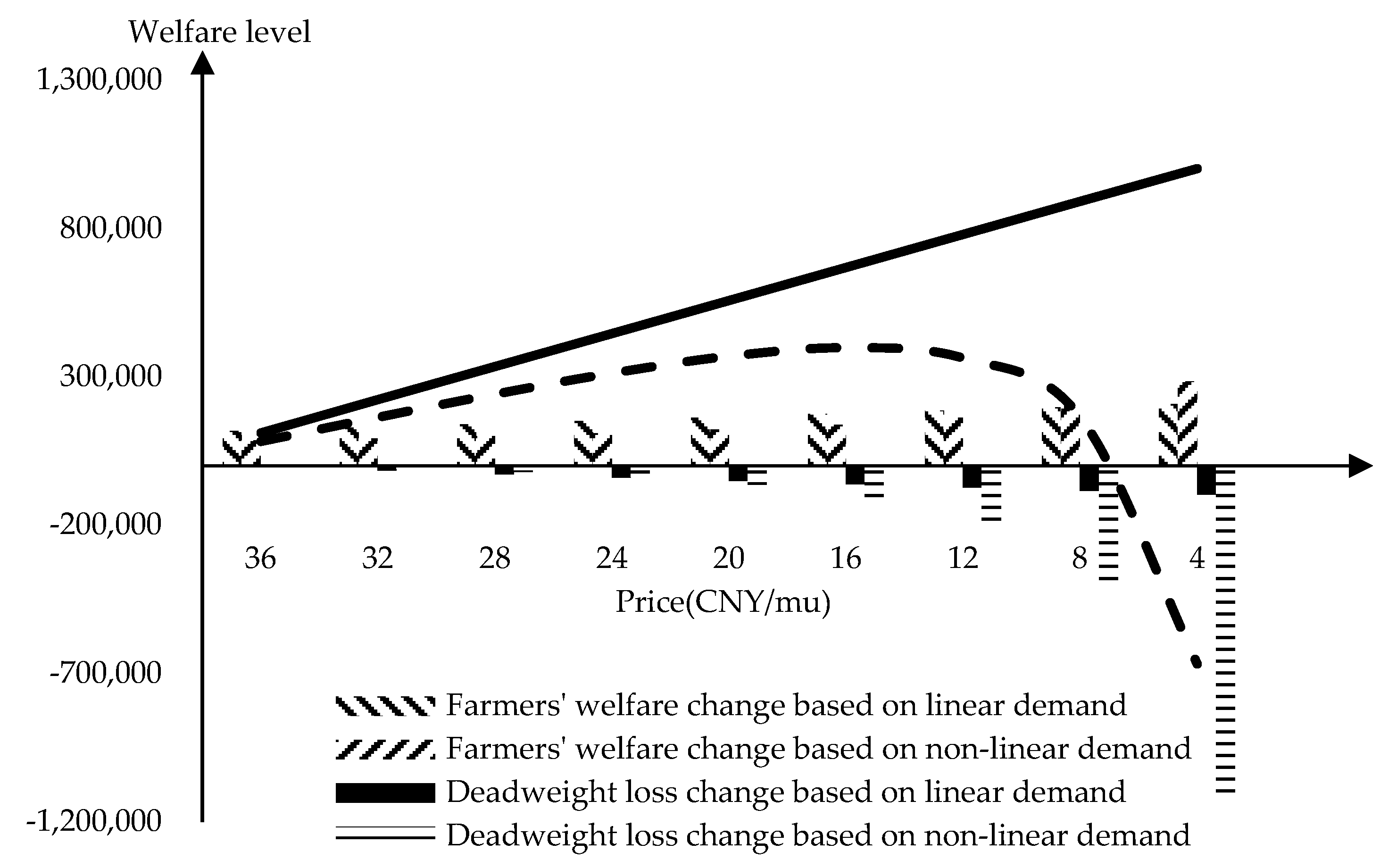
3.1. Regression Results and Welfare Measurement

The linear and power-law demand models for new insurance were estimated utilizing linear least-squares and nonlinear iterative methods, respectively. The estimated parameters are presented in detail in

Table 3. Parameter estimation based on planting area.

Parameter	Linear Demand	Power-Law Demand
	$\mathit{Q}=\mathit{a}+\mathit{b}\mathit{P}$	$\mathit{Q}=\mathit{a}{\mathit{P}}^{\mathit{b}}$
$a$	56,300.840 ***	220,326.600 ***
	(2308.652)	(25,035.180)
$b$	−711.647 ***	−0.642 ***
	(51.318)	(0.045)
$R^2$	0.861	0.970
$Adjust{R}^2$	0.857	0.968

Notes: Standard errors are in parentheses, *** p < 0.01. The table reports the parameter fitting results of linear distribution model and power law distribution model with cultivated land area as the demand unit. $R^2$ and the adjusted $R^2$ represent goodness of fit, and the larger the value, the better the goodness of fit.

, wherein the adjusted goodness-of-fit $R^2$ of the linear model is 0.857, while the adjusted goodness-of-fit $R^2$ of the power-law model reaches 0.968, suggesting that the power-law function more accurately characterizes the actual demand for crop insurance.

Through model fitting, we demonstrate that crop insurance demand exhibits greater consistency with the power-law function. Based on these estimates, the study measures the problem of changing welfare effects due to changes in the proportion of subsidies based on the relevant equation in the previous section.

Table 4. Welfare changes under different demand models.

Subsidy Level	Linear Demand					Power-Law Demand
	Farmers’ Welfare Change ${∆\mathit{C}\mathit{S}}_1$	Deadweight Loss Change ${∆\mathit{D}\mathit{W}\mathit{L}}_1$	${\mathit{g}}_1$	Total Welfare Effect	Welfare Effect Change ${∆\mathit{C}\mathit{S}}_1-{∆\mathit{D}\mathit{W}\mathit{L}}_1$	Farmers’ Welfare Change ${∆\mathit{C}\mathit{S}}_2$	Deadweight Loss Change ${∆\mathit{D}\mathit{W}\mathit{L}}_2$	${\mathit{g}}_2$	Total Welfare Effect	Welfare Effect Change ${∆\mathit{C}\mathit{S}}_2-{∆\mathit{D}\mathit{W}\mathit{L}}_2$
10%	117,033	5693	20.56	111,340	111,340	85,407	2972	28.74	82,434	82,434
20%	128,419	17,080	7.52	222,680	111,340	91,737	10,521	8.72	163,650	81,216
30%	139,806	28,466	4.91	334,019	111,340	99,427	21,477	4.63	241,600	77,950
40%	151,192	39,852	3.79	445,359	111,340	109,019	38,023	2.87	312,596	70,996
50%	162,578	51,239	3.17	556,699	111,340	121,406	64,393	1.89	369,609	57,014
60%	173,965	62,625	2.78	668,039	111,340	138,193	109,740	1.26	398,062	28,453
70%	185,351	74,011	2.50	779,379	111,340	162,612	197,193	0.82	363,481	−34,581
80%	196,737	85,398	2.30	890,719	111,340	202,518	401,657	0.50	164,342	−199,139
90%	208,124	96,784	2.15	1,002,058	111,340	284,844	1,117,149	0.25	−667,962	−832,304

Notes: The table reports the welfare changes with different subsidy levels under the assumption of linear demand and nonlinear demand. The specific figures can only represent the welfare changes and have no practical significance. Under the insurance products utilized in this study, each 10% increase in premium subsidy would result in a CNY 4 per mu reduction in premiums.

presents the specific results.

Under a linear demand model, increasing the premium subsidy enhances the subsidy’s welfare effect and benefits farmers to a greater extent than the subsidy welfare loss. The study utilizes the ratio $g$ to quantify the impact of subsidy on welfare effects. At a 10% subsidy, the ratio $g_1$ of new farmers’ welfare to new deadweight loss is 20.6, transferring over 95% of benefits to farmers. At a 90% subsidy, $g_1$ drops to 2.15, yet still transfers nearly 70% of benefits to farmers. This indicates that, while the subsidy increases the total welfare of farmers, the subsidy’s welfare effect diminishes as the level of subsidy increases, which validates research Hypothesis 1. Overall, at least half of the benefits of the subsidy accrue to farmers, rendering increased subsidy a viable approach to improve farmers’ welfare under the linear demand assumption.

In the power law demand model for crop insurance, the linear demand conclusions are not applicable (Figure 4). The welfare effect of subsidies does not increase consistently with increasing subsidies; it increases only at low levels of subsidies, and once subsidies exceed a certain threshold, the deadweight loss outweighs the increase in farmers’ welfare and increases rapidly, resulting in an inverted U-shaped trend in the welfare effect of subsidies, which validates Hypothesis 2. As demonstrated in Table 4, the ratio $g_2$ decreases with subsidy levels, reaching a maximum of 28.7 with a 10% premium subsidy and plummeting to 0.25 at a 90% subsidy, which further suggests that as the subsidy ratio increases, the welfare gains per unit of subsidy will be much lower than the welfare losses caused by the subsidy, greatly reducing the welfare effect of the subsidy.

Under the power law demand model, at a 60% subsidy level, the increased level of farmers’ welfare is approximately equivalent to the additional deadweight loss. Further increasing the subsidy ratio results in a decline in total welfare effect. In the study area, if subsidies exceed 80%, the total deadweight loss surpasses farmers’ welfare, indicating that, while subsidies enhance farmers’ welfare, they also negatively impact the overall welfare effect. To maximize farmers’ welfare without decreasing the welfare effect, the pursuit of further increases in premium subsidy would be counterproductive.

3.2. Robustness Test

In this section, we validate the demand for crop insurance utilizing the number of farmers purchasing crop insurance as an indicator. Supplementary Table S1 presents the estimated parameters. The adjusted $R^2$ for the linear model is 0.801 and the adjusted $R^2$ for the power-law model is 0.963. The same conclusion was reached using the amount of cropland area as the unit of demand, indicating that the power-law function more accurately represents the actual demand function for crop insurance.

We continue to apply the theoretical formulas from the previous section to evaluate the welfare effect of premium subsidy.

Table 5. Welfare changes under different demand models accounting for farmers as demand units.

Subsidy Level	Linear Demand					Power-Law Demand
	Farmers’ Welfare Change ${∆\mathit{C}\mathit{S}}_1$	Deadweight Loss Change ${∆\mathit{D}\mathit{W}\mathit{L}}_1$	${\mathit{g}}_1$	Total Welfare Effect	Welfare Effect Change ${∆\mathit{C}\mathit{S}}_1-{∆\mathit{D}\mathit{W}\mathit{L}}_1$	Farmers’ Welfare Change ${∆\mathit{C}\mathit{S}}_2$	Deadweight Loss Change ${∆\mathit{D}\mathit{W}\mathit{L}}_2$	${\mathit{g}}_2$	Total Welfare Effect	Welfare Effect Change ${∆\mathit{C}\mathit{S}}_2-{∆\mathit{D}\mathit{W}\mathit{L}}_2$
10%	531	29	8.31	502	502	366	14	26.14	352	352
20%	588	86	6.84	1004	502	397	51	7.78	698	346
30%	645	143	4.51	1507	502	434	106	4.09	1026	328
40%	703	200	3.52	2009	502	482	190	2.54	1318	292
50%	760	258	2.95	2511	502	544	326	1.67	1536	218
60%	817	315	2.59	3013	502	630	564	1.12	1602	66
70%	874	372	2.35	3515	502	757	1035	0.73	1324	−278
80%	932	429	2.17	4018	502	969	2170	0.45	123	−1201
90%	989	487	2.03	4520	502	1425	6324	0.23	−4776	−4899

Notes: The table reports the welfare promotion effect of different subsidy levels under the assumption of linear demand model and nonlinear demand model with farmer households as the demand unit. The specific figures can only represent the welfare change and have no practical significance. Under the insurance products utilized in this study, each 10% increase in premium subsidy would result in a CNY 4 per mu reduction in premiums.

demonstrates that the impact of an increased premium subsidy on enhancing the subsidy’s welfare effect remains limited. In the linear demand model, the total welfare effect increases concomitantly with the increase in the subsidy percentage. Conversely, in the power-law demand model, total welfare effect exhibits an inverted U-shaped trend as the subsidy rate increases. Total welfare effect reaches its maximum when the subsidy rate is approximately 60%. At a subsidy rate of approximately 80%, the total increase in farmers’ welfare attributable to the subsidy is approximately equivalent to the total deadweight loss in social welfare resulting from the premium subsidy.

In the model that measures crop insurance demand by the number of purchasing farmers, the primary conclusions derived from both the linear and power-law demand functions align with those from the demand model measured in mu. Specifically, under the linear demand model, both farmer welfare and the total welfare effect increase with the addition of a crop insurance premium subsidy. In the power-law demand model, farmer welfare also increases with the subsidy rate, albeit at a significantly slower rate than the increase in deadweight loss, resulting in an inverted U-shaped trend in total welfare effect. Furthermore, in both models, the welfare pull effect of an additional subsidy diminishes as the subsidy increases.

3.3. Heterogeneity Analysis

3.3.1. Regional Heterogeneity

Factors such as the frequency of natural disasters and income levels influence crop insurance demand, with farmers in high-risk areas attributing greater value to it and more affluent farmers exhibiting a higher likelihood of affording it. Consequently, it is imperative to comprehend the welfare impact of the premium subsidy across various regions. Distinct estimates for crop insurance demand curves in different cities have been calculated, with results presented in Supplementary Table S2.

The fitted model is used to calculate the change in welfare effects at different premium subsidy rates by region, with findings detailed in

Table 6. Welfare changes over cities.

Subsidy Level	Suqian City				Yancheng City				Huai’an City
	Farmers’ Welfare Change $∆\mathit{C}\mathit{S}$	Deadweight Loss Change $∆\mathit{D}\mathit{W}\mathit{L}$	${\mathit{g}}_{\mathit{s}}$	Total Welfare Effect	Farmers’ Welfare Change $∆\mathit{C}\mathit{S}$	Deadweight Loss Change $∆\mathit{D}\mathit{W}\mathit{L}$	${\mathit{g}}_{\mathit{y}}$	Total Welfare Effect	Farmers’ Welfare Change $∆\mathit{C}\mathit{S}$	Deadweight Loss Change $∆\mathit{D}\mathit{W}\mathit{L}$	${\mathit{g}}_{\mathit{h}}$	Total Welfare Effect
10%	11,131	380	29.29	10,751	29,397	911	32.28	28,486	46,982	1688	27.83	45,294
20%	11,940	1343	8.89	21,348	31,331	3201	9.79	56,617	50,580	5988	8.45	89,886
30%	12,921	2738	4.72	31,532	33,662	6478	5.20	83,801	54,962	12,254	4.49	132,594
40%	14,143	4839	2.92	40,836	36,541	11,355	3.22	108,987	60,442	21,758	2.78	171,277
50%	15,718	8178	1.92	48,376	40,219	19,004	2.12	130,202	67,543	36,976	1.83	201,844
60%	17,847	13,903	1.28	52,321	45,139	31,931	1.41	143,410	77,202	63,279	1.22	215,767
70%	20,936	24,904	0.84	48,354	52,181	56,356	0.93	139,235	91,320	114,311	0.80	192,776
80%	25,965	50,509	0.51	23,810	63,445	112,009	0.57	90,671	114,537	234,526	0.49	72,787
85%	16,195	48,726	0.33	−8720	38,785	105,961	0.37	23,495	72,262	228,771	0.32	−83,721
90%	36,281	139,515	0.26	−79,424	47,158	193,482	0.24	−122,829	90,635	431,193	0.21	−424,280

Notes: The table reports the welfare promotion effect of different subsidy levels under the assumption of linear demand model and nonlinear demand model in different cities. The specific figures can only represent the welfare change and have no practical significance.

. Suqian, Yancheng, and Huai’an cities have approximately 7899 mu, 18,132 mu, and 35,616 mu of land under cultivation by farmers interested in new wheat insurance, respectively.

The data indicate that welfare trends remain consistent across municipalities as the subsidy rate increases, and that subsidies can have a positive welfare effect in the agricultural production sector when the subsidy rate reaches 80%. However, when the subsidy rate reaches 90%, the total deadweight losses due to over-subsidization exceed the welfare it provides to farmers, resulting in significant inefficiencies in subsidies. It is noteworthy that only Yancheng maintains a positive welfare effect at an 85% subsidy rate, while the other cities experience a decline. Yancheng demonstrates higher welfare contribution efficiency, indicated by a higher ratio $g$, compared to Suqian and Huai’an. Within each subsidy interval, Yancheng’s ratio $g$ exceeds those of the other cities, except for a slight decrease when the subsidy increases from 85% to 90%, where it falls marginally below Suqian.

3.3.2. Risk Appetite Heterogeneity

Farmers’ risk preferences influence their propensity to purchase crop insurance. In comparison to risk-averse farmers, risk-preferring farmers exhibit a greater inclination to implement novel technologies in agricultural production, expand their farming operations, and experiment with new crop varieties. However, the expansion of scale, adoption of new technologies, and introduction of new varieties entail uncertainty, thereby increasing the risks associated with agricultural production. Consequently, risk-preferring farmers, in contrast to their risk-averse counterparts, have a greater need for crop insurance to safeguard their agricultural production and are likely to demonstrate a higher WTP for such insurance.

Based on this premise, this study employs an experimental design similar to that of Brick and Visser’s study [58] to determine farmers’ risk preference types through choice experiments. The specific experimental procedure is illustrated in Supplementary Table S6. Through this choice experiment, farmers are classified into three categories: risk-averse, risk-seeking, and risk-neutral.

Upon fitting the crop insurance demand model regression to the three categories of farmers with distinct risk preferences, it was observed that the crop insurance demand curve characteristics of these three farmer types align more closely with the power law distribution model. The specific fitting results are presented in Supplementary Table S3.

The results presented in the table demonstrate that the distribution of crop insurance demand exhibits characteristics consistent with a power law distribution. Furthermore, the $R^2$ and adjusted $R^2$ values of the power law fitting results for crop insurance demand across the three farmer categories are substantially higher than those obtained from the linear demand model. Utilizing the fitted models, the study conducts a further analysis of the welfare access for the three farmer categories under varying premium subsidy rates, as well as the differential welfare effects of the subsidies. Based on the derived model, the welfare changes for each farm household category are calculated, and the results are presented in

Table 7. Welfare changes under different risk attitudes.

Subsidy Level	Risk-Averse				Risk-Neutral				Risk-Seeking
	Farmers’ Welfare Change $∆\mathit{C}\mathit{S}$	Deadweight Loss Change $∆\mathit{D}\mathit{W}\mathit{L}$	${\mathit{g}}_{\mathit{a}\mathit{v}}$	Total Welfare Effect	Farmers’ Welfare Change $∆\mathit{C}\mathit{S}$	Deadweight Loss Change $∆\mathit{D}\mathit{W}\mathit{L}$	${\mathit{g}}_{\mathit{n}\mathit{e}}$	Total Welfare Effect	Farmers’ Welfare Change $∆\mathit{C}\mathit{S}$	Deadweight Loss Change $∆\mathit{D}\mathit{W}\mathit{L}$	${\mathit{g}}_{\mathit{s}\mathit{e}}$	Total Welfare Effect
10%	33,627	1426	23.58	32,202	15,748	539	29.23	15,209	30,129	853	35.33	29,276
20%	36,681	5118	7.17	63,764	16,895	1905	8.87	30,199	31,936	2982	10.71	58,230
30%	40,452	10,629	3.81	93,587	18,286	3884	4.71	44,602	34,101	5999	5.68	86,332
40%	45,244	19,194	2.36	119,637	20,020	6865	2.92	57,757	36,758	10,441	3.52	112,650
50%	51,569	33,272	1.55	137,935	22,254	11,605	1.92	68,406	40,127	17,332	2.32	135,445
60%	60,364	58,322	1.04	139,978	25,276	19,734	1.28	73,948	44,592	28,832	1.55	151,205
70%	73,576	108,599	0.68	104,955	29,661	35,361	0.84	68,248	50,910	50,249	1.01	151,866
75%	44,276	132,958	0.33	16,272	17,232	45,133	0.38	40,347	28,830	67,500	0.43	113,196
80%	51,827	188,172	0.28	−120,073	19,572	61,184	0.32	−1265	32,038	88,456	0.36	56,778
85%	63,170	292,402	0.22	−349,305	22,967	90,291	0.25	−68,589	36,578	125,352	0.29	−31,997
90%	82,510	534,043	0.15	−800,838	28,498	154,328	0.18	−194,419	43,732	203,474	0.21	−191,739

Notes: The table reports the welfare promotion effect of different subsidy levels under the assumption of linear demand model and nonlinear demand model in different cities. The specific figures can only represent the welfare change and have no practical significance.

.

To analyze more effectively the impact of differences in risk preferences on the welfare effects of crop insurance subsidies, the study is stratified into 5% increments, com-mencing from a subsidy ratio of 70%. The findings indicate that the welfare effects of the subsidy for both risk-averse and risk-neutral farmers are negative until the proportion exceeds 75%, whereas the welfare effects for risk-seeking farmers are negative until the proportion exceeds 80%. This confirms the previous hypothesis that risk-seeking farmers are more likely to take risks in the agricultural production process and therefore need crop insurance more to reduce risks.

3.3.3. Planting Scale Heterogeneity

The size of a farmer’s farm has a significant impact on his propensity to take out crop insurance. Compared with small-scale farmers, large-scale farmers are more vulnerable to natural disasters due to their large area under cultivation and are therefore more likely to need crop insurance to mitigate the effects of natural disasters. In this study, based on China’s agricultural producer classification standard, farmers with more than 50 hectares of cultivated area are classified as large-scale farmers, and farmers with less than 50 hectares of cultivated area are classified as small-scale farmers. The results of the model fitting (Supplementary Table S4) show that the distribution of crop insurance demand for large and small agricultural producers has consistent power law distribution characteristics. Using the fitted model, this study further analysed the differences between the two types of agricultural producers. Based on the derived model, the welfare changes for each type of agricultural household were calculated and the results are presented in

Table 8. Welfare changes under different planting scales.

Subsidy Level	Smallholder				Large-Scale Household
	Farmers’ Welfare Change $∆\mathit{C}\mathit{S}$	Deadweight Loss Change $∆\mathit{D}\mathit{W}\mathit{L}$	${\mathit{g}}_{\mathit{a}\mathit{v}}$	Total Welfare Effect	Farmers’ Welfare Change $∆\mathit{C}\mathit{S}$	Deadweight Loss Change $∆\mathit{D}\mathit{W}\mathit{L}$	${\mathit{g}}_{\mathit{n}\mathit{e}}$	Total Welfare Effect
10%	1841	74	24.96	1767	84,908	2868	29.61	82,040
20%	1998	264	7.58	3502	91,011	10,131	8.98	162,920
30%	2192	545	4.03	5149	98,408	20,633	4.77	240,695
40%	2437	977	2.49	6609	107,611	36,431	2.95	311,875
50%	2758	1682	1.64	7684	119,462	61,502	1.94	369,835
60%	3201	2923	1.09	7961	135,464	104,413	1.30	400,886
70%	3859	5385	0.72	6436	158,642	186,718	0.85	372,810
75%	2299	6654	0.35	2082	91,990	239,042	0.38	225,759
80%	2668	9306	0.29	−4556	104,312	323,272	0.32	6799
85%	3218	14,255	0.23	−15,593	122,161	475,685	0.26	−346,725
90%	4142	25,560	0.16	−37,012	151,160	810,049	0.19	−1,005,614

Notes: The table reports the welfare promotion effect of different subsidy levels under the assumption of linear demand model and nonlinear demand model in different cities. The specific figures can only represent the welfare change and have no practical significance.

.

This section is similarly divided into bands of 5%, commencing from a 70% subsidy ratio. The results indicate that the welfare effect of premium subsidies for small farmers becomes negative at subsidy rates exceeding 75%, while for large farmers, it becomes negative at subsidy rates exceeding 80%. This trend is also reflected in the subsidy efficiency, which consistently demonstrates higher values for large farmers compared to small farmers. Nevertheless, the three heterogeneity analyses reveal that although differences exist in the welfare effects between the various groups, the percentage of difference is approximately 5%, suggesting that the overall crop insurance requirements of farmers are low. However, the proportion of subsidies at which the welfare effect is maximized remains consistent for both small and large farmers, reaching its peak at approximately 60% of the subsidy. It is noteworthy that the welfare effect for large farmers decreases at a slower rate than that for small farmers.

4. Discussion

The extent of the welfare effect of increased crop insurance premium subsidies remains a subject of debate. Certain studies have posited that the increase in premium subsidies has effectively promoted the adoption of crop insurance and increased farmers’ risk tolerance, enabling them to enhance their investments in new machinery, agricultural materials, and seeds, etc. [59,60,61]. However, other studies have demonstrated that the continuously increasing scale of premium subsidies has augmented the financial burden on the government without effectively increasing the actual insurance needs of farmers, resulting in significant inefficiencies in resource allocation [62,63]. Furthermore, research has indicated that due to the risk underwriting of crop insurance, farmers have cultivated a large number of insured crops, leading to distortions in the supply and demand dynamics of the crop market, which may potentially compromise national food security. Conner and Katchova’s study [64] revealed that the increase in crop insurance participation rates led to farmers expanding cultivation into low-quality farmland, paradoxically resulting in an increased risk of yield decline. Additionally, Miao’s study [65] found that the risk diversification mechanism of crop insurance exhibits a crowding-out effect on other risk management instruments, thereby inhibiting the long-term capacity of society to adapt to climate change.

Indeed, the actual demand for crop insurance by farmers partially determines the magnitude of the welfare effect of insurance subsidies. Tsiboe and Turner’s study [66] demonstrates that the elasticity of demand for crop insurance by farmers increases with a reduction in subsidies but does not further explore the welfare distribution of subsidies. In addition, existing studies also lack models that can reasonably describe the real demand for crop insurance among farmers. Therefore, our study first clarifies the model that can accurately describe the distribution of real demand for crop insurance among farmers, which compensates for the lack of a reasonable model for the distribution of real demand for crop insurance in existing studies. At the same time, the study also discusses in detail the impact of changes in the level of premium subsidies on the distribution of welfare, and by deriving the calculation of the welfare effect of subsidies, it refutes the stereotype that an increase in premium subsidies can continuously bring about a large amount of welfare improvement in the agricultural production sector, and provides strong theoretical and empirical results to support policy makers.

5. Conclusions

The purpose of this study is to examine the impact of crop insurance premium subsidy rates on farmers’ welfare, subsidy loss, and subsidy welfare effects, with the aim of exploring the actual distribution of farmers’ demand for crop insurance and the appropriate range of crop insurance premium subsidy. Through the constructed theoretical model combined with empirical analyses, this study confirms the power law distribution characteristics of farmers’ crop insurance and draws the following main conclusions: First, the demand for crop insurance in China is more in line with power law distribution characteristics, and its long-tailed nature suggests that the majority of farmers do not have high demand for crop insurance. Second, there is an inverted U-shaped trend between the proportion of crop insurance premium subsidy and the welfare effect of the subsidy, and when the subsidy exceeds a certain proportion, the welfare effect of the subsidy falls off a cliff, causing a large welfare loss. Third, the heterogeneity of farm households leads to differences in the welfare effects of subsidies, but the differences caused by such heterogeneity are not significant.

This study innovatively introduces the power law distribution model to the crop insurance market, which breaks the usual linear demand model assumption in traditional insurance demand research. Meanwhile, through theoretical analysis and derivation, the study reasonably verifies that the power law distribution model can truly describe the distribution of farmers’ demand for crop insurance. In addition, the study provides mathematical modelling support for the relationship between the premium subsidy rate and the subsidy welfare effect, which is a missing part in previous subsidy welfare studies. We also show through empirical modelling that changes in the welfare distribution of premium subsidies differ from the findings of previous studies, which in effect refutes the optimistic view that increased premium subsidies can consistently generate positive welfare effects in the agricultural sector and provides a basis for policy makers.

It is important to note that this study measures the relationship between the level of premium subsidy and the welfare effect of subsidies through mathematical and econometric models based on supply and demand in the insurance market. However, other external factors such as market access issues, agricultural inputs, food production stability, and welfare spillovers were not included in the welfare analysis model, which is a limitation of this study. Future research should include more relevant factors in the welfare analysis model of this study and also consider the combined welfare effects of premium subsidies, so that the overall impact of premium subsidies on social welfare can be analyzed on the basis of the welfare effects of premium subsidies by analyzing the impact of premium subsidies on different sectors.

References

1. Wagner, K.R.H. Designing Insurance for Climate Change. Nat. Clim. Chang. 2022, 12, 1070–1072. [Google Scholar] [CrossRef]
2. Gao, Y.; Shu, Y.; Cao, H.; Zhou, S.; Shi, S. Fiscal Policy Dilemma in Resolving Agricultural Risks: Evidence from China’s Agricultural Insurance Subsidy Pilot. Int. J. Environ. Res. Public Health 2021, 18, 7577. [Google Scholar] [CrossRef]
3. Guo, Y.M.; Shi, Y.R. Impact of the VAT Reduction Policy on Local Fiscal Pressure in China in Light of the COVID-19 Pandemic: A Measurement Based on a Computable General Equilibrium Model. Econ. Anal. Policy 2021, 69, 253–264. [Google Scholar] [CrossRef]
4. Fang, L.; Hu, R.; Mao, H.; Chen, S. How Crop Insurance Influences Agricultural Green Total Factor Productivity: Evidence from Chinese Farmers. J. Clean. Prod. 2021, 321, 128977. [Google Scholar] [CrossRef]
5. Yang, X.; Liu, Y.; Bai, W.; Liu, B. Evaluation of the Crop Insurance Management for Soybean Risk of Natural Disasters in Jilin Province, China. Nat. Hazards 2015, 76, 587–599. [Google Scholar] [CrossRef]
6. Yu, J.; Smith, A.; Sumner, D.A. Effects of Crop Insurance Premium Subsidies on Crop Acreage. Am. J. Agric. Econ. 2018, 100, 91–114. [Google Scholar] [CrossRef]
7. Wang, K.; Zhang, Q.; Kimura, S.; Akter, S. Is the Crop Insurance Program Effective in China? Evidence from Farmers Analysis in Five Provinces. J. Integr. Agric. 2015, 14, 2109–2120. [Google Scholar] [CrossRef]
8. Schaffitzel, F.; Jakob, M.; Soria, R.; Vogt-Schilb, A.; Ward, H. Can Government Transfers Make Energy Subsidy Reform Socially Acceptable? A Case Study on Ecuador. Energy Policy 2020, 137, 111120. [Google Scholar] [CrossRef]
9. Fadhliani, Z.; Luckstead, J.; Wailes, E.J. The Impacts of Multiperil Crop Insurance on Indonesian Rice Farmers and Production. Agric. Econ. 2019, 50, 15–26. [Google Scholar] [CrossRef]
10. Gassler, B.; Rehermann, R. Risk Preferences and the Adoption of Subsidised Crop Insurance: Evidence from Lithuania. Ger. J. Agric. Econ. 2022, 71, 36–52. [Google Scholar] [CrossRef]
11. Sharma, S.; Walters, C.G. Influence of Farm Size and Insured Type on Crop Insurance Returns. Agribusiness 2020, 36, 440–452. [Google Scholar] [CrossRef]
12. Hou, D.; Wang, X. Inhibition or Promotion?–The Effect of Agricultural Insurance on Agricultural Green Development. Front. Public Health 2022, 10, 910534. [Google Scholar] [CrossRef]
13. Yan, F.; Yi, F.; Chen, H. Effect of Education on Crop Insurance Knowledge: Evidence from a RCT in China. China Agric. Econ. Rev. 2024. [Google Scholar] [CrossRef]
14. Ricome, A.; Affholder, F.; Gérard, F.; Muller, B.; Poeydebat, C.; Quirion, P.; Sall, M. Are Subsidies to Weather-Index Insurance the Best Use of Public Funds? A Bio-Economic Farm Model Applied to the Senegalese Groundnut Basin. Agric. Syst. 2017, 156, 149–176. [Google Scholar] [CrossRef]
15. Zhang, R.; Ma, W.; Liu, J. Impact of Government Subsidy on Agricultural Production and Pollution: A Game-Theoretic Approach. J. Clean. Prod. 2021, 285, 124806. [Google Scholar] [CrossRef]
16. Ye, T.; Wang, M.; Hu, W.; Liu, Y.; Shi, P. High Liabilities or Heavy Subsidies: Farmers’ Preferences for Crop Insurance Attributes in Hunan, China. China Agric. Econ. Rev. 2017, 9, 588–606. [Google Scholar] [CrossRef]
17. Ramirez, O.A.; Carpio, C.E. Are the Federal Crop Insurance Subsidies Equitably Distributed? Evidence from a Monte Carlo Simulation Analysis. J. Agric. Resour. Econ. 2015, 40, 457–475. [Google Scholar] [CrossRef]
18. Alizamir, S.; Iravani, F.; Mamani, H. An Analysis of Price vs. Revenue Protection: Government Subsidies in the Agriculture Industry. Manag. Sci. 2019, 65, 32–49. [Google Scholar] [CrossRef]
19. Yang, T.; Li, Z.; Bai, Y.; Liu, X.; Ye, T. Residents’ Preferences for Rural Housing Disaster Insurance Attributes in Central and Western Tibet. Int. J. Disaster Risk Sci. 2023, 14, 697–711. [Google Scholar] [CrossRef]
20. Zhong, L.; Nie, J.; Yue, X.; Jin, M. Optimal Design of Agricultural Insurance Subsidies under the Risk of Extreme Weather. Int. J. Prod. Econ. 2023, 263, 108920. [Google Scholar] [CrossRef]
21. Okubo, M. Model Uncertainty, Economic Development, and Welfare Costs of Business Cycles. J. Macroecon. 2023, 76, 103514. [Google Scholar] [CrossRef]
22. Mazzoleni, P.; Pagani, E.; Perali, F. On the Curvature Properties of “Long” Social Welfare Functions. Mathematics 2023, 11, 1674. [Google Scholar] [CrossRef]
23. Ohdoi, R.; Futagami, K. Welfare Implications of Non-Unitary Time Discounting. Theory Decis. 2021, 90, 85–115. [Google Scholar] [CrossRef]
24. Huang, J.-C.; Zhao, M.Q. Model Selection and Misspecification in Discrete Choice Welfare Analysis. Appl. Econ. 2015, 47, 4153–4167. [Google Scholar] [CrossRef]
25. Vercammen, J.; Pannell, D.J. The Economics of Crop Hail Insurance. Can. J. Agri. Econ. 2000, 48, 87–98. [Google Scholar] [CrossRef]
26. Hill, R.V.; Kumar, N.; Magnan, N.; Makhija, S.; De Nicola, F.; Spielman, D.J.; Ward, P.S. Ex Ante and Ex Post Effects of Hybrid Index Insurance in Bangladesh. J. Dev. Econ. 2019, 136, 1–17. [Google Scholar] [CrossRef]
27. Yi, F.; Zhou, M.; Zhang, Y.Y. Value of Incorporating ENSO Forecast in Crop Insurance Programs. Am. J. Agric. Econ. 2020, 102, 439–457. [Google Scholar] [CrossRef]
28. Heyne, P.; Boettke, P.; Prychitko, D.L. The Economic Way of Thinking; Science Research Associates: Chicago, IL, USA, 1987. [Google Scholar]
29. Rubinstein, M. An Aggregation Theorem for Securities Markets. J. Financ. Econ. 1974, 1, 225–244. [Google Scholar] [CrossRef]
30. Dai, J.; Meng, W. A Risk-Averse Newsvendor Model under Marketing-Dependency and Price-Dependency. Int. J. Prod. Econ. 2015, 160, 220–229. [Google Scholar] [CrossRef]
31. Lynch, M.Á.; Nolan, S.; Devine, M.T.; O’Malley, M. The Impacts of Demand Response Participation in Capacity Markets. Appl. Energy 2019, 250, 444–451. [Google Scholar] [CrossRef]
32. Stark, O.; Budzinski, W. A Social-psychological Reconstruction of Amartya Sen’s Measures of Inequality and Social Welfare. Kyklos 2021, 74, 552–566. [Google Scholar] [CrossRef]
33. Zou, H. The Social Welfare Effect of Environmental Regulation: An Analysis Based on Atkinson Social Welfare Function. J. Clean. Prod. 2024, 434, 140022. [Google Scholar] [CrossRef]
34. Ahmed, S.; McIntosh, C.; Sarris, A. The Impact of Commercial Rainfall Index Insurance: Experimental Evidence from Ethiopia. Am. J. Agric. Econ. 2020, 102, 1154–1176. [Google Scholar] [CrossRef]
35. Cole, S.; Fernando, A.N.; Stein, D.; Tobacman, J. Field Comparisons of Incentive-Compatible Preference Elicitation Techniques. J. Econ. Behav. Organ. 2020, 172, 33–56. [Google Scholar] [CrossRef]
36. Palm-Forster, L.H.; Swinton, S.M.; Shupp, R.S. Farmer Preferences for Conservation Incentives That Promote Voluntary Phosphorus Abatement in Agricultural Watersheds. J. Soil Water Conserv. 2017, 72, 493–505. [Google Scholar] [CrossRef]
37. Khalid, S.A.; Salman, V. Welfare Impact of Electricity Subsidy Reforms in Pakistan: A Micro Model Study. Energy Policy 2020, 137, 111097. [Google Scholar] [CrossRef]
38. Wang, Y.; Lin, B. Performance of Alternative Electricity Prices on Residential Welfare in China. Energy Policy 2021, 153, 112233. [Google Scholar] [CrossRef]
39. Goolsbee, A. The Value of Broadband and the Deadweight Loss of Taxing New Technology. Contrib. Econ. Anal. Policy 2006, 5, 0000101515153806451505. [Google Scholar] [CrossRef]
40. Anderson, S.P.; Renault, R. Efficiency and Surplus Bounds in Cournot Competition. J. Econ. Theory 2003, 113, 253–264. [Google Scholar] [CrossRef]
41. Berry-Stölzle, T.R. Evaluating Liquidation Strategies for Insurance Companies. J. Risk Insur. 2008, 75, 207–230. [Google Scholar] [CrossRef]
42. Zhu, X.; Van Ommeren, J.; Rietveld, P. Indirect Benefits of Infrastructure Improvement in the Case of an Imperfect Labor Market. Transp. Res. Part B Methodol. 2009, 43, 57–72. [Google Scholar] [CrossRef]
43. Pinto, C.M.A.; Mendes Lopes, A.; Machado, J.A.T. A Review of Power Laws in Real Life Phenomena. Commun. Nonlinear Sci. Numer. Simul. 2012, 17, 3558–3578. [Google Scholar] [CrossRef]
44. Rozenfeld, H.D.; Rybski, D.; Gabaix, X.; Makse, H.A. The Area and Population of Cities: New Insights from a Different Perspective on Cities. Am. Econ. Rev. 2011, 101, 2205–2225. [Google Scholar] [CrossRef]
45. Bulut, H. Managing Catastrophic Risk in Agriculture through Ex Ante Subsidized Insurance or Ex Post Disaster Aid. J. Agric. Resour. Econ. 2017, 42, 406–426. [Google Scholar]
46. Amoah, A.; Ferrini, S.; Schaafsma, M. Electricity Outages in Ghana: Are Contingent Valuation Estimates Valid? Energy Policy 2019, 135, 110996. [Google Scholar] [CrossRef]
47. Chen, Q.; Liu, G.; Liu, Y. Can Product-Information Disclosure Increase Chinese Consumer’s Willingness to Pay for GM Foods? The Case of Fad-3 GM Lamb. China Agric. Econ. Rev. 2017, 9, 415–437. [Google Scholar] [CrossRef]
48. Drichoutis, A.C.; Lusk, J.L.; Pappa, V. Elicitation Formats and the WTA/WTP Gap: A Study of Climate Neutral Foods. Food Policy 2016, 61, 141–155. [Google Scholar] [CrossRef]
49. Orlowski, J.; Wicker, P. Monetary Valuation of Non-Market Goods and Services: A Review of Conceptual Approaches and Empirical Applications in Sports. Eur. Sport Manag. Q. 2019, 19, 456–480. [Google Scholar] [CrossRef]
50. Heinzen, R.R.; Bridges, J.F.P. Comparison of Four Contingent Valuation Methods to Estimate the Economic Value of a Pneumococcal Vaccine in Bangladesh. Int. J. Technol. Assess. Health Care 2008, 24, 481–487. [Google Scholar] [CrossRef]
51. Bageant, E.R.; Barrett, C.B. Are There Gender Differences in Demand for Index-Based Livestock Insurance? J. Dev. Stud. 2017, 53, 932–952. [Google Scholar] [CrossRef]
52. Islam, M.D.I.; Rahman, A.; Sarker, M.N.I.; Sarker, M.S.; Jianchao, L. Factors Influencing Rice Farmers’ Risk Attitudesand Perceptions in Bangladesh amidEnvironmental and Climatic Issues. Pol. J. Environ. Stud. 2020, 30, 177–187. [Google Scholar] [CrossRef] [PubMed]
53. Tang, Y.; Cai, H.; Liu, R. Farmers’ Demand for Informal Risk Management Strategy and Weather Index Insurance: Evidence from China. Int. J. Disaster Risk Sci. 2021, 12, 281–297. [Google Scholar] [CrossRef]
54. Goodwin, B.K. An Empirical Analysis of the Demand for Multiple Peril Crop Insurance. Am. J. Agric. Econ. 1993, 75, 425–434. [Google Scholar] [CrossRef]
55. Kim, Y.; Yu, J.; Pendell, D.L. Effects of Crop Insurance on Farm Disinvestment and Exit Decisions. Eur. Rev. Agric. Econ. 2019, 47, 324–347. [Google Scholar] [CrossRef]
56. Lusk, J.L. Distributional Effects of Crop Insurance Subsidies. Appl. Econ. Perspect. Policy 2017, 39, 1–15. [Google Scholar] [CrossRef]
57. Hagquist, C.; Stenbeck, M. Goodness of Fit in Regression Analysis—R2 and G2 Reconsidered. Qual. Quant. 1998, 32, 229–245. [Google Scholar] [CrossRef]
58. Brick, K.; Visser, M. Risk Preferences, Technology Adoption and Insurance Uptake: A Framed Experiment. J. Econ. Behav. Organ. 2015, 118, 383–396. [Google Scholar] [CrossRef]
59. Ward, P.S.; Ortega, D.L.; Spielman, D.J.; Kumar, N.; Minocha, S. Demand for Complementary Financial and Technological Tools for Managing Drought Risk. Econ. Dev. Cult. Change 2020, 68, 607–653. [Google Scholar] [CrossRef]
60. Philippi, T.; Schiller, J. Abandoning Disaster Relief and Stimulating Insurance Demand through Premium Subsidies. J. Risk Insur. 2024, 91, 339–382. [Google Scholar] [CrossRef]
61. Wong, H.L.; Wei, X.; Kahsay, H.B.; Gebreegziabher, Z.; Gardebroek, C.; Osgood, D.E.; Diro, R. Effects of Input Vouchers and Rainfall Insurance on Agricultural Production and Household Welfare: Experimental Evidence from Northern Ethiopia. World Dev. 2020, 135, 105074. [Google Scholar] [CrossRef]
62. Qin, T.; Gu, X.; Tian, Z.; Pan, H.; Deng, J.; Wan, L. An Empirical Analysis of the Factors Influencing Farmer Demand for Forest Insurance: Based on Surveys from Lin’an County in Zhejiang Province of China. J. For. Econ. 2016, 24, 37–51. [Google Scholar] [CrossRef]
63. Glauber, J.W. Crop Insurance Reconsidered. Am. J. Agri. Econ. 2004, 86, 1179–1195. [Google Scholar] [CrossRef]
64. Connor, L.; Katchova, A.L. Crop Insurance Participation Rates and Asymmetric Effects on U.S. Corn and Soybean Yield Risk. J. Agric. Resour. Econ. 2020, 45, 1–19. [Google Scholar] [CrossRef]
65. Miao, R. Climate, Insurance and Innovation: The Case of Drought and Innovations in Drought-Tolerant Traits in US Agriculture. Eur. Rev. Agric. Econ. 2020, 47, 1826–1860. [Google Scholar] [CrossRef]
66. Tsiboe, F.; Turner, D. The Crop Insurance Demand Response to Premium Subsidies: Evidence from U.S. Agriculture. Food Policy 2023, 119, 102505. [Google Scholar] [CrossRef]
Figure 1. Linear demand model. Figure 1 constructs a linear demand model for crop insurance based on a market equilibrium model, where the diagonal line AH represents aggregate farmer demand and BI, FE, and GH represent market supply at different insurance prices.
Agriculture 14 02050 g001
Figure 2. Non-linear demand model. Figure 2 constructs a power law distribution demand model for crop insurance based on the market equilibrium model, where the curves represent aggregate farmer demand and BF, AC, and DE represent market supply at different insurance prices.
Agriculture 14 02050 g002
Figure 3. Demand for crop insurance in the survey area.
Agriculture 14 02050 g003
Figure 4. Welfare changes under different demand models. The solid line in the figure represents the level of the welfare effect of the premium subsidy ratio under a linear crop insurance demand model, while the dashed line represents the level of the welfare effect of the premium subsidy ratio under a power-law distribution demand model.
Agriculture 14 02050 g004