Multi-Scenario Simulation of Optimal Landscape Pattern Configuration in Saline Soil Areas of Western Jilin Province, China

Abstract

The Songnen Plain is a significant region in China, known for its high grain production and concentrated distribution of soda saline land. It is also considered a priority area for cropland development in the country. However, the Songnen Plain is now facing prominent issues such as soil salinization, soil erosion, and deteriorating cropland quality, which are exacerbated by climate change and intensified human activities. In order to address these challenges, it is crucial to adjust the quantitative structure and layout of different landscapes in a harmonious manner, aiming to achieve synergistic optimization, which is posed as the key scientific approach to guide comprehensive renovation policies, improve saline–alkaline land conditions, and promote sustainable agricultural development. In this study, four scenarios including natural development, priority food production (PFP), ecological security priority (ESP), and economic–ecological-balanced saline soil improvement were set up based on Nondominated Sorting Genetic Algorithm II (NSGA-II) and the Future Land Use Simulation (FLUS) model. The results demonstrated that the SSI scenario, which focused on economic–ecological equilibrium, displayed the most rational quantitative structure and spatial layout of landscape types, with total benefits surpassing those of the other scenarios. Notably, this scenario involved converting unused land into saline cropland and transforming saline cropland into normal cropland, thereby increasing the amount of high-quality cropland and potential cropland while enhancing the habitat quality of the region. Consequently, the conflict between food production and ecological environmental protection was effectively mitigated. Furthermore, the SSI scenario facilitated the establishment of a robust ecological security and protection barrier, offering valuable insights for land use planning and ecological security pattern construction in the Songnen Plain, particularly in salt-affected areas.

1. Introduction

The saline soil area in western Jilin Province plays a crucial role in ensuring sustained grain production in China. However, this region is frequently subjected to wind, sand, salinization, and droughts, leading to the deterioration of black soil cropland quality [1]. The high concentration of soluble salts in the soil has further exacerbated the decline in agricultural land quality, inhibiting crop growth and resulting in extensive barren and wasteland formation. This not only hampers ecological environments but also poses significant challenges to agricultural development [2,3]. In recent years, local authorities have prioritized the improvement of saline soils and the prevention of secondary salinization. Effective strategies for enhancing land resource utilization, promoting the conversion of improved saline soils, restoring agricultural productivity, and ensuring food production are key factors in guiding scientifically grounded policies. These policies are essential for effectively addressing the comprehensive rehabilitation and sustainable development of saline soils while preserving ecosystem diversity and stability [4].

Landscape pattern optimization entails the efficient allocation of land resources among various sectors within a specific region, while adhering to specific constraints, and aiming to achieve maximum benefits with regard to ecological, social, and economic aspects. Specifically, Cao et al. [5] and Shu et al. [6] focused on pattern optimization for land use in urban agglomerations and sustainable agricultural development in the North China Plain, respectively. Wang et al. [7] proposed a methodology to optimize the quantitative structure of land use types and rationalize their spatial arrangement by employing scientific techniques. The research of Luan et al. [8] demonstrated that earlier multi-objective optimization methods often relied on subjective weighting of objectives and the integration of multiple sub-objective functions into a single one based on experience. Yang et al. [9] utilized mathematical models and multi-objective optimization techniques to address the landscape pattern configuration problem. Pan et al. [10] and Wu et al. [11] argued that single objective functions had limitations, including subjective weight assignment and a lack of alternative solutions. In addition, Makowski et al. [12] utilized a linear programming model to simulate the development of agricultural land use. However, it was challenging for the linear programming model to comprehensively and quantitatively analyze the intricate land use structure. Similarly, Huo et al. [13] optimized land use in the Xiongan New Area using a Markov model. Nevertheless, their model is not suitable for forecasting over long time series in the future. After evaluating the urban growth of Shanghai City, Han et al. [14] discovered that the system dynamics model must specify the various feedback mechanisms within the system to ensure accurate simulation results. Furthermore, some scholars have also integrated computer algorithms with goal optimization problems to propose heuristic algorithms, such as simulated annealing algorithms [15], particle swarm algorithms [16], and genetic algorithms [17]. These algorithms can efficiently optimize the solutions of multi-objective functions. However, the algorithms above may also encounter challenges such as insufficient diversity and slow convergence speed [18,19].

With the depth of research, scholars have proposed a series of optimization models to enhance the landscape pattern. The primary objective of landscape pattern optimization is to maximize the comprehensive benefit value of land within a specific scope, essentially simulating future land use [20]. Prominent models in this domain include the CLUE (Conversion of Land Use and its Effect) model, CA (Cellular Automata) model, and FLUS (Future Land Use Simulation) model. Particularly, the CLUE model presents a dynamic modeling framework formulated by Veldkmap and Fresco [21] in 1996, commonly employed for simulating large-scale land use changes. However, the calculation of the CLUE model is often oversimplified, primarily due to the empirical statistical parameters that heavily rely on researchers’ experiences. As a grid dynamics model, the CA model is utilized for spatially simulating a specific site type. However, the CA model is often combined with linear programming for spatial layout optimization [22]. Nevertheless, previous landscape pattern studies based on the CA model primarily focused on estimating the conversion probabilities of different land types, without adequately considering the limiting roles and competitive relationships among these classes in predictive landscape pattern simulations [23]. Recognizing the limitations of the traditional CA model, Liu et al. [24] proposed the FLUS model. This model incorporates adaptive inertia and competition mechanisms to address complex competition and interaction issues among land types, and has proven to be effective in simulating various landscape pattern scenarios [25,26]. Specifically, the FLUS model integrates the multifaceted influences of human activities and natural processes, utilizes the Back Propagation Artificial Neural Network (BP-ANN) to calculate land suitability probabilities, and combines the CA model to establish an adaptive inertia and competition mechanism capable of capturing the intricate competition and interactions among land use types such as cropland, forest, grassland, waters, built-up areas, and unused land [27,28,29]. Consequently, the FLUS model has been widely employed in landscape pattern simulations, exhibiting a satisfactory level of accuracy with Kappa coefficients above 0.75 [30,31,32].

The western region of Jilin is one of the three major global distributions of soda saline–alkali soil, which has been plagued by soil salinization for a long time, restricting the self-restoration of the ecological environment in the study area and threatening the improvement of grain economic productivity. However, saline soil also possesses high potential productivity and can be transformed into productive soil, such as paddy fields, grasslands, and wetlands, through improvement measures. Scientifically planning and allocating salinized areas with human intervention to achieve a balanced development between grain production and ecological environmental protection is of great significance for preventing secondary soil salinization and promoting sustainable land resource utilization. Based on land use trends over the past three decades and future government planning documents, we formulated four potential future development directions. The objectives of this study are (1) to investigate how the landscape quantity allocation and spatial pattern in the study area will change by 2030 under these four scenarios; and (2) based on the aforementioned results and the need to achieve multi-objective trade-offs, how do we select the optimal development scenario for 2030?

2. Material and Methods

2.1. Study Area

The western part of Jilin Province is located in the southwestern part of the Songnen Plain, belonging to the low-lying and flood-prone saline–alkaline land and wind–sand land landscape-intertwined area, covering an area of about 4.7 × 10⁴ km², with a geographic location between 121°30′–121°37′ E longitude and 43°59′–46°28′ N latitude. The western region of Jilin is characterized by a low-lying central area with higher elevations on both sides, and is dotted with numerous rivers and lakes. Additionally, the soil types (Figure 1) in this region are diverse, with Chernozem and Phaeozem being widely distributed (accounting for 38.71% and 27.51% of the total study area, respectively). Arenosol and Solonchak are interspersed in the southwestern part of the study area (accounting for 13.81% and 8.24% of the total study area, respectively). In this study, two municipal administrative districts were contained, including Baicheng City (Taobei District, Da’an City, Taonan City, Zhenlai County, and Tongyu County) and Songyuan City (Fuyu City, Qian Guo County, Changling County, and Qian’an County). Due to the agricultural and animal husbandry activities in the intertwined zone, economic development of western Jilin is primarily centered around plantation and tertiary industries. As a result, there has been a growing demand for improved land quality. However, the available land resources are unable to meet these economic demands, leading to the over-cultivation of certain areas. Consequently, the quality of the habitat has declined, aggravated by spring droughts and secondary soil salinization. These factors have intensified the conflict between human activities and the land, further amplifying the human–land contradiction.

2.2. Data Sources

The specific data types used in this study are shown in

Table 1. Data source information.

Data Type	Data Content		Data Source
Land Use Data	Land use data of Jilin Province from 1990 to 2020		Data Center for Resources and Environmental Sciences, Chinese Academy of Sciences (http://www.resdc.cn/) (accessed on 26 November 2024)
Satellite Image Data	Landsat-5 TM, Landsat-8 OLI		NASA (https://earthexplorer.usgs.gov/) (accessed on 26 November 2024)
Statistical Almanac Data	Industrial output value by administrative region from 1990 to 2020		Jilin bureau of Jilin statistics yearbook (http://tjj.jl.gov.cn/tjsj/tjnj/) (accessed on 26 November 2024)
Planning Text Data	Master Plan of Baicheng Land Space (2021–2035), Master Plan of Songyuan City (2021–2035)		Baicheng City People’s Government (http://www.jlbc.gov.cn/) (accessed on 26 November 2024) Songyuan Municipal People’s Government (https://www.jlsy.gov.cn/) (accessed on 26 November 2024)
Driving Force Factor Data	Natural factors	DEM	NASA (https://earthexplorer.usgs.gov/)
		Temperature, precipitation	Data Center for Resources and Environmental Sciences, Chinese Academy of Sciences (http://www.resdc.cn/) (accessed on 26 November 2024)
	Transport accessibility factor	Distance to rail, road	OSM (https://www.openstreetmap.org/) (accessed on 26 November 2024)
	Socio-economic factors	Population density per unit area	World pop (https://www.worldpop.org/) (accessed on 26 November 2024)
		GDP data of China’s kilometer grid	National Earth System Science Data Center (http://www.geodata.cn/) (accessed on 26 November 2024)

. Based on satellite imagery and field measurement samples, a saline soil identification model was constructed. Starting from the inversion of saline soil areas in the western region of Jilin Province, and considering their overlap with the primary land use categories of cropland, forest, and grassland, three new land use categories were ultimately derived: saline cropland, saline forest, and saline grassland. Figure 2a represents the extent of saline soil; (b) shows the primary land use categories of cropland, forest, and grassland; and (c) displays the results of the new land use categories after overlaying (a) and (b).

In this study, the land use data were processed using a level 1 classification system to obtain information on the nine land use categories relevant to the study area (

Table 2. Land use type classification system standard.

Land Use Type Classification System	Land Use Type
CNLUCC Classification System	Cropland, forest, grassland, waters, built-up land, unused land
Spatial classification system of “Three life”	Production space land (cropland, industrial, and mining construction land), Ecological space land (forest, waters, unused land), Living space land (urban and rural living land)
The classification system of this study	Cropland, forest, grassland, waters, built-up land, unused land, Saline cropland *, saline forest *, saline grassland *

* Additional land use category.

). Subsequently, specific land use areas were identified and combined with government planning documents to establish the relevant constraints and scenarios for the study. To evaluate the economic benefits of each land use category, the coefficients of the objective function were calculated using data from the Statistical Yearbook. Additionally, the coefficients of the ecological benefit objective function were calibrated with reference to the ecological value service equivalence table based on Xie et al. [33], which were thus applied to the NSGA-II algorithm as setting parameters.

After determining the land classification system for the study area, we selected common driving factor data that influence the development and changes in saline–alkali land in the western region of Jilin. Natural factors determine the physical suitability of land, transportation accessibility affects the economic value and development potential of land, and socio-economic factors reflect the direct and indirect demands of human activities on land use. Therefore, we selected seven data points from three dimensions—natural (temperature, precipitation, DEM), transportation accessibility (distance to road, distance to railway), and socio-economic (population density, GDP)—as the driving factors for simulating landscape types using the FLUS model (Figure 3).

2.3. Methods

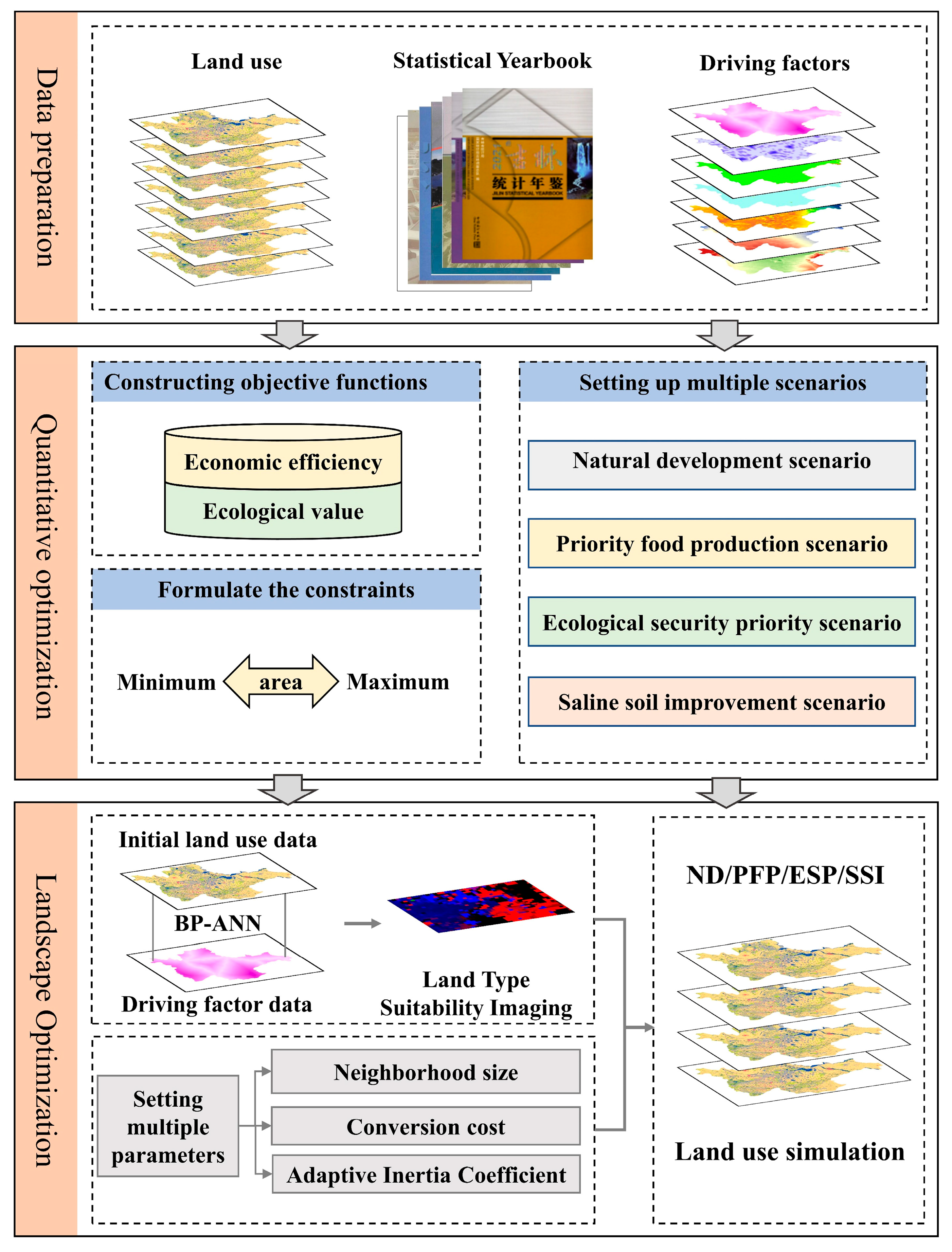
2.3.1. Research Framework

Figure 4 illustrates the flow-process diagram utilized in this study, suggesting that the main data comprise three essential components such as land use data, satellite images, and driver factors. Initially, the land use data and satellite images were merged to identify and delineate the saline soil area. Furthermore, an objective function for the NSGA-II algorithm was established based on the ecological value service table and Statistical Yearbook data. Moreover, relevant land constraints were determined based on governmental textual information. Four development scenarios (ND, PFP, ESP, and SSI scenarios) were formulated. Specifically, the ND scenario was created employing the Markov chain module of GeoSOS-FLUS V2.4, while the other three scenarios were designed using the NSGA-II algorithm. Additionally, data for seven driving factors were selected, and the FLUS model was employed to allocate image elements of each class under multiple scenarios within the study area. In the year 2030, the changes and differences in the quantitative structure of land use, the outcomes of landscape optimization, and the value of total production benefits were analyzed for the various scenarios. Ultimately, the most suitable future development scenario for landscape optimization in the region was selected after conducting a comparative analysis.

2.3.2. NSGA-II Algorithm

In this study, the NSGA-II algorithm was selected to address the optimization problem related to the future distribution of land use in areas with saline soil, which consists of three components such as the selection of decision variables, construction of objective functions, and formulation of constraints. In particular, nine decision variables corresponding to different land categories (cropland, forest, grassland, waters, built-up land, unused land, saline cropland, saline forest, saline grassland) were identified based on Table 2. After considering the demand for land resources for high-quality economic development in the study area, two objective functions including the economic benefit objective function and the ecological benefit objective function were then constructed. Additionally, the range of constraint thresholds was estimated and formulated based on government policy documents and the area distribution of different land categories in the study area, which embodies the restriction and protection of the land development in the process and can effectively alleviate the tension of land use in the area. It is worth noting that these constraint thresholds address the requirements for land development in the study process, resulting in a more balanced and rational land use structure. This ultimately helps mitigate regional land use tensions and allows for better control and adjustment of land utilization.

Objective Benefit Function Construction

(1) The economic benefit objective function is listed as follows:

$$max{F}_1={\displaystyle \sum }_{i=1}^n{A}_i{x}_i$$

(1)

where $F_1$ is the economic benefit, $n$ represents the number of land use types, $x_i$ is the area corresponding to each land use type, and $A_i$ refers to the value of the economic benefit coefficient and describes the economic output produced by the land use type $i$. Based on the ratio of social output to the area of the land type in the Jilin Statistical Yearbook, the economic benefit is obtained by calculating the economic benefit through the five-year coefficient and then using the Grey Model—GM—(1,1) to predict the value for the next five years.

(2) The ecological benefit objective function is listed as follows:

$$max{F}_2={\displaystyle \sum }_{i=1}^n{B}_i{x}_i$$

(2)

where $F_2$ is the ecological value, $n$ describes the number of land use types, $x_i$ is the area of each land use type, and $B_i$ refers to the ecological value coefficient, suggesting the eco-efficiency output value outputted by the land use type $i$. The coefficient was obtained by referring to China’s table of ecological service value coefficients, which was obtained by combining the average grain production and grain unit price in Jilin Province in the past 30 years, and the national subsidy standard for returning cropland to forest from 2002 to 2010. The above two types of objective function coefficients shown in

Table 3. Economic benefit coefficient and ecological benefit coefficient in saline soil area.

Function	C	F	G	W	B	U	S–C	S–F	S–G
Coefficient Ai	411.33	52.56	563.85	111.27	21,095.87	0	176.86	4.39	247.26
Coefficient Bi	295.35	1391.75	901.99	6640.84	0	48.60	169.73	72.02	47.53

C, cropland; F, forest; G, grassland; W, waters; B, build-up land; U, unused land; S-C, saline cropland; S-F, saline forest; S-G, saline grassland.

indicate that cropland, grassland, and built-up land have a more direct impact on the economic benefits, while forest and waters have a significant increase in the ecological benefits.

Development Scenario and Constraints

According to the economic development characteristics of saline soil improvement in western Jilin Province, four scenarios of future landscape pattern change in the saline soil area were set up with reference to urban planning. Future scenarios of the saline soil area in 2030 were also realized through the prediction of the area of each land use category in the demands of different scenarios with quantitative allocation simulation shown in

Table 4. Future development scenario setting.

Scenario Setting	Scenario Description	Land Class Conversion Requirements
ND	Follow the natural evolution law of land use type	There are no restrictions on the conversion between land types
PFP	Grain production is fundamentally in cropland, and the red line of cropland should be strictly observed The target weights of economic and ecological benefits are 0.8 and 0.2, respectively	Conversion of arable land and construction land to other land types is prohibited
ESP	Strengthen the protection of ecological land for waters’ environment, simulate the land structure with the highest ecological benefits, and ensure ecological development. The target weights of economic benefit and ecological benefit are 0.2 and 0.8, respectively	The conversion of forest land and waters’ area to other land types is prohibited. Arable land and grassland can be converted to geographical areas of higher ecological value
SSI	Steadily accelerate saline soil to improve soil with normal salt content and increase its agricultural utilizable value. The target weights of economic benefit and ecological benefit are 0.5 and 0.5, respectively	The conversion of other land types into unused land shall be prohibited, and the conversion of unused land into economic and ecological land shall be vigorously developed

.

In this study, decision-making constraints including the cropland constraint (x₁), forest constraint (x₂), grassland constraint (x₃), waters’ constraint (x₄), built-up land constraint (x₅), unused land constraint (x₆), saline cropland constraint (x₇), saline forest constraint (x₈), saline grassland constraint (x₉), and non-negative constraint on decision-making volume (x_i) were determined from the perspectives of total land area constraint C. All constraints can reflect the requirements of the economic development and ecological environment in western Jilin Province, and thus be used to realize the maximum–minimum regulation of government planning on the area of land resources (

Table 5. The area constraint of land use type.

Constraint Type	Constraints/km2	Instructions
Total land area constraint C	$C={\displaystyle {\displaystyle \sum }_{i=1}^9}{x}_i$	The sum of the planned area (xi) of each land use type shall be equal to the total area C of the study area
Cropland area constraint (x1)	24,851.08 ≤ x1 ≤ 25,219.62	The minimum size of cropland shall not be lower than the current status of cropland in 2020, and the maximum size shall be set with the growth rate of cropland from 1990 to 2020
Forest area constraint (x2)	2796.09 ≤ x2 ≤ 3142.98	The minimum size of the forest land should not be lower than the current situation of the forest land area in 2020, and the maximum size should be set up by 10% according to the development trend of 1990–2020
Grassland area constraint (x3)	4531.99 ≤ x3 ≤ 4812.31	The change in the grassland area is not only affected by human activities, but also greatly affected by rainfall. The change range of the grassland area is set as the base ±3% of the grassland area under the ND scenario
Waters’ area constraint (x4)	1966.33 ≤ x4 ≤ 2162.96	The minimum size of the waters’ area is not lower than the 2020 status quo. And the maximum is set to increase the waters’ area by 10% in 2020
Built-up land area constraint (x5)	1815.43 ≤ x5 ≤ 1967.57	The minimum scale of construction land shall not be lower than the controlled amount of the construction land scale in 2020. The maximum scale is set with the growth rate of construction land from 1990 to 2020
Unused land area constraint (x6)	8734.51 ≤ x6 ≤ 9653.93	Set the unused land area change range as the base ± 5% of the unused land area under the ND scenario
Saline cropland land area constraint (x7)	578.51 ≤ x7 ≤ 737.01	The minimum scale of saline cropland is the current situation of saline cropland in 2020, and the maximum scale is set by the improvement rate of saline cropland from 1990 to 2020
Saline forest area constraint (x8)	56.90 ≤ x8 ≤ 88.56	The minimum scale of saline forest land is the current situation of the saline forest land area in 2020, and the maximum scale is set as the improvement speed of saline forest land
Saline grassland area constraint (x9)	418.36 ≤ x9 ≤ 426.82	The change range of the saline grassland area is set to be ± 1% of the area at the rate of improvement of the saline grassland
Non-negative constraint of decision quantity (xi)	xi ≥ 0, i = 1, 2, 3, 4, 5, 6, 7, 8, 9	In the model, each constraint variable is required to be non-negative

).

2.3.3. FLUS Model

In this study, the FLUS model was selected to simulate future changes in landscape patterns in the saline soil area. The FLUS model consists of two components. The first component involves the use of the BP-ANN algorithm to determine the probability of appropriateness for different types of land use. This is achieved by analyzing historical land use data, as well as multiple driving factors. The second component of the FLUS model involves the use of the CA model, which utilizes an adaptive inertia competition mechanism to simulate the layout outcomes.

Calculate Suitability Probability Based on BP-ANN Algorithm

The BP-ANN algorithm is employed to calculate the sustainability probability. It is trained using multiple iterations of historical land use data and various driving factors influencing its changes. This process aims to enhance the dataset’s fitting accuracy and compute the grid suitability probability, $p\left(p,k,t\right)$, for the corresponding land resource’s land use. The specific equation of $p\left(p,k,t\right)$ is listed as follows:

$$\begin{gathered} p\left(p,k,t\right)={\displaystyle \sum }_j{w}_{j,k}\times sigmoid\left(ne{t}_j\left(p,t\right)\right) \\ \hspace{1em}={\displaystyle {\displaystyle \sum }_j}{w}_{j,k}\times {\displaystyle \frac{1}{1+e^{-net}{j}^{\left(p,t\right)}}} \end{gathered}$$

(3)

where $p\left(p,k,t\right)$ is the adaptive probability of different land use types $k$ in a saline soil area at training time $t$ for unit grid $p;$ $w_{j,k}$ are the adaptive weights between the hidden layer and the output layer in different contexts, with its sum considered as 1. The $sigmoid$ describes the activation function from the hidden layer to the output layer; and $ne{t}_j\left(p,t\right)$ denotes the suitability demand received by the $j$th hidden layer grid $p$ at training time $t$, and the probability of grid cell suitability for the nine land use types.

CA Model Based on Adaptive Inertial Competition Mechanism

The core of the adaptive inertia competition mechanism is considered as the adaptive inertia coefficient, which is adjusted during the simulation iterations to move the quantities of each land use type towards the specified demand target based on the suitability probability results mentioned above, and the raster data of each land use type in different scenarios of saline soil landscapes. The adaptive inertia coefficient is computed using the formula below:

$$Interti{a}_k^{t }=\left\{\begin{array}{cc}Interti{a}_k^{t-1}\hfill & \hspace{1em}\left|D_k^{t-1}\right| \le \left|D_k^{t-2}\right|\\ Interti{a}_k^{t-1}\times {\displaystyle \frac{D_k^{t-2}}{D_k^{t-1}}}\hfill & \hspace{1em}{D}_k^{t-1}<D_k^{t-2}<0\\ Interti{a}_k^{t-1}\times {\displaystyle \frac{D_k^{t-1}}{D_k^{t-2}}}\hfill & \hspace{1em}0<D_k^{t-2}<D_k^{t-1}\end{array}\right.$$

(4)

where $D_k^{t-1}$ and $D_k^{t-2}$ represent the difference between the number of raster targets and the matching area for the different scenarios of class $k$ sites at 2030 and 2020, respectively.

The conversion probability of each land use class is then determined by the combination of the corresponding suitability probability, neighborhood size, conversion cost (whether to convert between classes), and adaptive inertia coefficients. After taking into account the various factors mentioned above, the following formula was carried out to calculate the overall conversion probability of the land use type raster:

$$TPro{b}_{p,k}^t=p\left(p,k,t\right)\times {\Omega }_{p,t}^t\times Interti{a}_k^t\times \left(1-s{c}_{c\to k}\right)$$

(5)

where $TPro{b}_{p,k}^t$ is the overall conversion probability of raster $p$ to be converted from other land types to site type $k$ in 2030, and $s{c}_{c\to k}$ is the cost of converting the original site type $c$ to the new site type $k$; $1-s{c}_{c\to k}$ denotes the ease with which the transformation occurs; ${\Omega }_{p,t}^t$ refers to the neighborhood effect representing the ability of the land use type to expand in the land transformation, calculated by Equation (6):

$${\Omega }_{p,k}^t={\displaystyle \frac{{\Sigma }_{N\times N}con\left(c_p^{t-1}=k\right)}{N\times N-1}}\times W_k$$

(6)

where ${\Sigma }_{N\times N}con\left(c_p^{t-1}=k\right)$ denotes the total number of rasters of the land use type $k$ class in Moore’s neighborhood window of $N\times N$ after $t-1$ iterations, which is taken to be $N$ = 5 in this study, and $W_k$ refers to the weight of the intensity of the neighborhood effect for each land use type.

2.3.4. Precision Evaluation

The Kappa coefficient was selected to assess the accuracy of land use classification with its formula shown as follows:

$$k={\displaystyle \frac{P_0-P_c}{1-P_c}}$$

(7)

where $P_0$ represents the overall accuracy of the simulation results; $P_c$ refers to the correct rate of simulation for each grid in the random state. The Kappa coefficient ranges from 0 to 1, with higher values indicating more accurate classification results. In general, a Kappa coefficient more than 0.75 is usually selected to carry out the simulation prediction with high accuracy.

3. Results and Discussion

3.1. Validation of Land Use Simulation

In this study, salinization land use data and related driving factor data were combined to obtain the land use simulation results in 2020 (Figure 4), which were validated with the real land use. It can be seen from the figure that the model realistically reflected the land use changes in western Jilin Province and can be used in the study area for the simulation and prediction of future land use with a Kappa coefficient of 0.8.

3.2. Structure Analysis Under Different Scenario Configurations

In order to quantitatively analyze the changes in land area between 2020 and 2030, a statistical analysis was conducted on the gains and losses of different land types in various scenarios. The findings are presented in

Table 6. Changes in area gains and losses under different scenarios.

Land Class	2020/km2	2030/km2
		ND		PFP		ESP		SSI
		S	△S	S	△S	S	△S	S	△S
Cropland	24,851.08	25,868.81	1017.73	25,215.5	364.42	24,920.79	69.71	25,045.01	193.93
Forest	2796.09	2600.10	−195.99	2893.34	97.25	3138.43	342.34	3063.34	267.25
Grassland	4437.86	4672.15	234.29	4777.14	339.28	4802.99	365.13	4808.33	370.47
Waters	1966.33	1555.24	−411.09	2008.57	42.24	2162.96	196.63	2113.78	147.45
Built-up land	1815.43	1675.31	−140.12	1967.57	152.14	1893.81	78.38	1952.55	137.12
Unused land	10,096.31	9494.22	−602.09	9053.87	−1042.44	9005.99	−1090.32	8873.46	−1222.85
Saline cropland	578.51	626.32	47.81	682.55	104.04	660.44	81.93	728.34	149.83
Saline forest	56.90	54.65	−2.25	56.90	0	65.73	8.83	68.05	11.15
Saline grassland	478.50	530.21	51.71	421.57	−56.93	425.87	−52.63	424.15	−54.35

. Specifically, under the ND (no development) scenario, the area of cropland and grassland exhibited an increasing trend, with an increase of 1017.73 km² and 234.29 km², respectively, compared to 2020. On the other hand, the areas of forest land, waters, construction land, and unused land all showed a decreasing trend. Among them, the forest area decreased by 195.99 km², the waters’ area decreased by 411.09 km², the construction land area decreased by 140.12 km², and the unused land area decreased by 602.09 km². However, the changes in the area of saline cropland, saline forest land, and saline grassland were relatively small. It is important to note that the ND scenario was formulated based on historical land change inertia and was driven by both natural and socio-economic factors, without considering the influence of policy factors. Thus, the above results can be considered as meeting the requirements of the scenario setting.

Table 6 also demonstrates that the regularizing PFP (protection of cropland policy) scenario exhibited an increasing trend in the predicted area of cropland, forest land, grassland, construction land, and saline cropland. Compared to 2020, the predicted cropland area for 2030 increased by 364.42 km², the forest land area increased by 97.25 km², the grassland area increased by 339.28 km², the construction land area increased by 152.14 km², and the saline cropland area increased by 104.04 km². Meanwhile, the unused land area in 2030 decreased by 1042.44 km² compared to 2020. Furthermore, there was a slight decrease in the area of waters, saline forests, and saline grasslands. In order to strictly implement the policy of cropland protection and adhere to the red line of cropland in western Jilin Province, the expansions of cropland and saline cropland were considered as the main focus under the PFP scenario. However, the transfer and conversion of cropland and construction land to other land types were limited.

Regarding the ESP scenario, the projected areas of forest, grassland, and waters in 2030 all exhibited an increasing trend compared to 2020. Specifically, the forest area expanded by 342.34 km², grassland increased by 365.13 km², and waters’ area increased by 196.63 km². Conversely, there was a significant reduction in the extent of unused land, amounting to a decrease of 1090.32 km² by 2030. Nevertheless, the variations in the areas of cropland, construction land, saline cropland, saline forest land, and saline grassland were relatively minimal. This outcome can be attributed to the emphasis placed on ecological security in the ESP scenario, wherein the expansion of construction land was restricted, the conversions of forests and waters to other land types were prohibited, and the geographical conversions of cropland and grasslands to areas with higher ecological value were facilitated.

Under the SSI scenario, the predicted areas of cropland, forest land, grassland, waters’ area, construction land, and saline cropland in 2030 displayed an increasing trend. Specifically, the cropland area expanded by 193.93 km², the forest area increased by 267.25 km², the grassland area increased by 370.47 km², the waters’ area increased by 147.45 km², the construction land area increased by 137.12 km², and the saline cropland area increased by 149.83 km². However, the changes in the areas of saline forests and saline grasslands were relatively minor. Furthermore, the SSI scenario witnessed the largest transfer of unused land among the four scenarios, amounting to 1222.85 km². In conclusion, it is evident that under the SSI scenario, a substantial amount of unused land has been developed, while other land types have experienced steady growth. This outcome aligned with the objective of accelerating soil improvement under the SSI scenario, facilitating regional economic development, and maintaining a balance between economic progress and ecological security.

In order to improve the understanding of the flow direction of land changes in different land classes, the transfer of various land classes under four scenarios from 2020 to 2030 was statistically analyzed, as depicted in Figure 5. It is evident from the figure that, under the ND scenario, there was a substantial loss of forest land, grassland, construction land, and unused land in 2020, which mainly converted into cropland. Additionally, some waters transitioned into grasslands. However, the transfer of cropland, saline cropland, saline forest land, and saline grassland was not significant. Regarding the PFP scenario, the lost unused land transformed into cropland, forest land, grassland, waters, construction land, and saline cropland. Furthermore, the outflow of forest land, grassland, and saline cropland predominantly converted into cropland. However, the flow of saline forest land and saline grassland was not significant under this scenario. As for the ESP scenario, the transfer of land types in various regions was primarily driven by the conversion of unused land into forest, grassland, and waters. Conversely, the flow of cropland, construction land, saline cropland, saline forest, and saline grassland was not significant. Furthermore, Figure 6 demonstrates that the SSI scenario exhibited a significant transfer of the area from unused land to saline cropland, while the outflow of forest land, grassland, and saline cropland mainly transitioned into cropland. Moreover, a considerable amount of saline grassland converted into grassland, but the flow of waters was not evident.

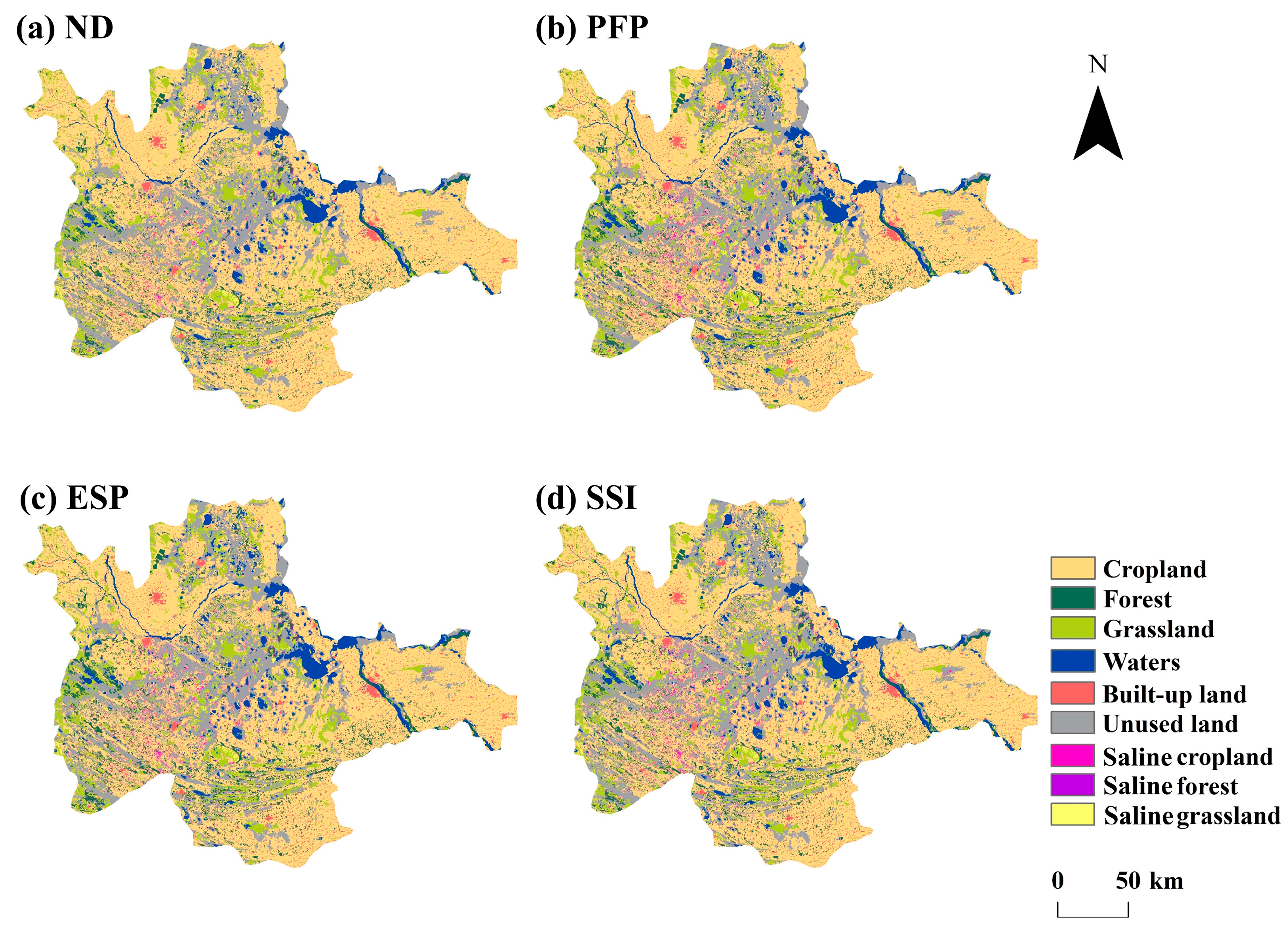
3.3. Landscape Pattern Analysis Under Four Scenario Configurations

Figure 7 presents the landscape optimization layout obtained by applying the land use quantity in the FLUS model. The graph indicates that, under the four different scenarios, cropland was widely spread throughout the study area, with forests and grasslands intersecting each other. Waters predominately concentrated in the middle of the study area, while construction land exhibited a limited aggregation state. Additionally, unused land was primarily distributed in the central and western regions, while saline cropland appeared sporadically near unused land. However, saline forests and grasslands were less prevalent in the study area.

In order to further clarify the land use changes between the actual pattern in 2020 and the simulation in 2030, a corresponding fluctuation trend under four scenarios was created in this study, as shown in Figure 8. Figure 8(a1,a2) demonstrate that under the ND scenario, there was a notable conversion of unused land in Taonan City, Da’an City, and Tongyu County into cropland. Moreover, there was an extensive degradation of waters in the study area, particularly in small areas dominated by the Moon Bubble. The waters of the Tao’er River flowing through Taonan City and Da’an City have also transitioned into cropland. Additionally, some reduced waters in Da’an City and Tongyu County have been transformed into grasslands, and certain forest lands in the border area between Taonan City and Da’an City have disappeared. The degradation of unused land in the study area was relatively evenly distributed, while changes in other land types were quite insignificant. Figure 8(b1,b2) reveal that under the PFP scenario, the distribution of arable land and construction land growth was relatively uniform. The expansion of cropland in this scenario was slightly lower than that in the ND scenario. Zhenlai County, Tongyu County, and Da’an City have experienced notable transformations from grassland and forest land to other land types. The expansion of waters’ area was concentrated in Da’an City. The area of saline cropland in Tongyu County and Qian’an County has increased significantly. Additionally, there has been a significant outflow of unused land within the study area. However, the changes in saline forest land and saline grassland were relatively insignificant. From Figure 8(c1,c2), it can be observed that under the ESP scenario, a substantial conversion of grassland appeared in Da’an City and Zhenlai County. Forest land was concentrated in the western part of Tongyu County. The water area in the region has experienced a significant expansion, with the Chagan Lake area expanding notably. Furthermore, there has been a small-scale expansion of waters, particularly in the Hua’ao Pao area, and in Qianguo County and Da’an City. The unused land in the study area has uniformly decreased on a large scale, while the other land types have not undergone significant changes. In addition, Figure 8(d1,d2) indicate that under the SSI scenario, the conversion of unused land into saline cropland was concentrated in the central and western parts of the study area. Cropland in Taonan City, Tongyu County, and Qianguo County has also experienced some changes, while other land types have remained relatively stable.

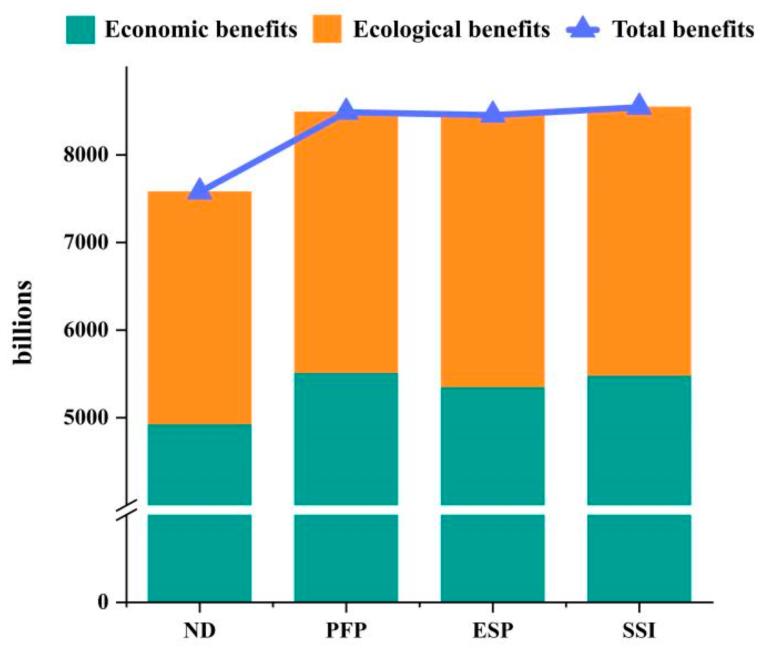
3.4. Comparative Analysis of Benefits

According to the function parameters of the NSGA-II algorithm, the economic and ecological benefits of four scenarios in the saline soil area of western Jilin were compared and analyzed (

Table 7. Comparison of multi-scenario benefits (CNY 100 million).

2030	ND	PFP	ESP	SSI
Economic benefits	4916.90	5517.39	5353.84	5483.39
Ecological benefits	2639.82	2970.17	3099.91	3061.47
Total benefits	7556.72	8487.56	8453.76	8544.86

). The table demonstrates that all four scenarios were optimized and transformed based on their respective conditions, incorporating appropriate adjustments to the quantity structure and landscape pattern, suggesting that this approach can effectively promote sustainable development in the region.

A further analysis of output benefits under different scenarios is presented in Figure 9. The findings indicate that the ND scenario yielded the lowest total benefit among all four scenarios, with economic and ecological benefits amounting to CNY 491.69 billion and CNY 263.982 billion, respectively. The PFP scenario stood out with the highest economic benefits of CNY 551.739 billion, accompanied by a slight improvement in ecological benefits. However, the PFP scenario did not surpass the ecological benefits achieved in the ESP and SSI scenarios. Specifically, the ESP scenario yielded an economic benefit of CNY 535.384 billion, while its ecological benefit reached the highest value among the four scenarios at CNY 309.991 billion. On the other hand, the SSI scenario generated a slightly lower economic benefit of CNY 548.339 billion compared to PFP; yet, its ecological benefit of CNY 306.147 billion remained on par with ESP. Consequently, when considering total benefits, the SSI scenario emerged as the most advantageous with CNY 854.486 billion.

4. Discussion

4.1. Impact of Different Scenarios on Landscape Patterns

Saline soil is a prevalent issue across China, posing a threat to the country’s food security and ecological balance. In recent years, substantial progress has been made in addressing saline soil in western Jilin Province through measures such as salt discharge, washing, and the cultivation of salt-tolerant crops [34]. To further improve understanding, four simulation scenarios were established in this study, specific to saline soil areas in Jilin Province. Given the province’s significance as a major grain-producing region, the impacts of expanding cultivated and saline lands on local economic development were emphasized by simulating landscape patterns. Consequently, the implications of various scenarios were examined from both economic and ecological perspectives on the landscape pattern of saline soil areas in western Jilin Province.

Without being subject to government macroeconomic regulation, a large amount of water and unused land in the ND scenario has turned into arable land, resulting in a severe degradation of water ecological land. This unregulated expansion infringes upon development space and poses a significant threat to ecological security. Without appropriate constraints and restrictions, the habitat quality in western Jilin will inevitably decline [35]. Furthermore, a development plan solely focused on increasing the area of cropland to boost regional GDP, disregarding other economic activities, undermines ecological security and contradicts the principles of sustainable planning, which thus exacerbates the conflict between human needs and land resources, hindering the sustainable development of the social economy.

During the implementation of PFP schemes, there was a varying degree of development on unused land. In addition, the PFP approach can slow down the rate of cropland conversion in comparison to the ND scenario, thereby ensuring a relatively healthy development trend in the regional economy. However, in the context of the rapid economic development in western Jilin Province, the expansion of construction land was still inevitable, with a majority of the transferred land being directed towards economic purposes. While this plan effectively alleviated conflicts in the landscape pattern of saline soil areas, it overlooked the serious ecological and environmental issues associated with such areas [36].

The prevalent distribution of saline soil in the research area highlights the fragility of the local ecosystem. Therefore, under the ESP scenario, there was a rapid development of ecological land, such as grasslands, forests, and waters, to ensure the preservation of the development space for ecological purposes. As compared to the PFP approach, the reduction in ecological land acquisition by construction land in the ESP scenario has a positive impact on maintaining the ecological security of the research area [37]. However, the ESP approach has a relatively singular focus on the conversion of ecological land and places greater emphasis on ecological benefits while sacrificing the economic benefits of the region.

The land use structure under the SSI scenario exhibited a relatively scientific distribution, with minimal amounts of unused land and saline land compared to the other three scenarios. The research area primarily focused on the transformation sequence of “unused land—saline cropland—cropland”. The transitions between different land categories were relatively gradual, maintaining a stable and sustainable pattern, predominantly building upon the existing distribution with a compact structure. The SSI scenario demonstrated high levels of both economic and ecological benefits, surpassing the other three scenarios in terms of total benefits. This made the SSI scenario align better with the current development objective of expanding the total economic output in the western region of Jilin Province. Additionally, it can meet the requirements for food production positioning while alleviating soil degradation resulting from ecological crises [38]. Therefore, the SSI scenario was deemed the most suitable future development approach for the research area and can provide valuable insights for landscape optimization and configuration in saline soil regions.

It is important to note that the other three scenarios, namely ND, PFP, and ESP, also have appropriate implementation sites based on their specific characteristics. For instance, the ND scenario adheres to historical evolution trends and is suitable for regions with a relatively underdeveloped economy or slower urbanization processes. Consequently, it entails minor adjustments and changes within the landscape pattern of the study area [39]. The PFP scenario prioritizes urban land expansion and is suitable for economically developed urban agglomerations with a greater demand for construction land [40]. Lastly, taking into account the important roles of forest, waters, and grassland in enhancing carbon sequestration, conserving soil and water, and maintaining biodiversity [41,42], as outlined in China’s ecological protection redline policy, we will ensure the necessary living spaces for these three types of land use in the ESP scenario. Therefore, it is more applicable to areas with sensitive and fragile ecological environments, with limited human intervention [43].

4.2. Comparison of Landscape Simulation Models

This study employed the FLUS model to address the issue of landscape simulation from a multi-objective trade-off perspective in saline soil areas. Among the currently mainstream landscape configuration models, the CA model boasts powerful computational capabilities but can only simulate the evolution of a single land use type. It is often coupled with models such as linear programming [44]; yet, it fails to capture the competitive relationships among the nine land use types in the study area. The CLUE-S model, while capable of comprehensively considering natural and human factors and quantifying the relationship between land use changes and driving factors [45], performs poorly in addressing adaptive changes in the land use system of saline soil areas. The PLUS model can automatically generate dynamic spatio-temporal simulated patches based on the expansion of various land use types [46]; however, it requires a large number of localized parameters, and the setting of these parameters significantly influences the simulation results, making it challenging to apply this model to address the issues in the study area. The FLUS model, on the other hand, can directly calculate the quantity of changes for different land use types based on historical evolution trends, offering high simulation accuracy and fast running speed [47]. However, it faces difficulties in reading high-resolution images or large-scale images of extensive areas, limiting its operational effectiveness. Given that the final output of this study is at a 100 m resolution, and considering the small study area and complex land use types, the FLUS model is deemed the most suitable choice.

4.3. Limitations of This Research

In the simulation of land allocation based on multiple scenarios, landscape pattern changes are influenced by numerous factors. However, this study only considers seven driving factors that were explicitly listed. Additionally, different driving factors also have significant interferences on the layout of land suitability. Furthermore, while the impact of economy and policies on land change is most pronounced in the short term, the underlying reasons are ultimately controlled by natural factors. On the other hand, due to limitations in model operation, it is challenging to calculate the land use of high-resolution images during the experimental process. Future research should aim to comprehensively consider the impact of improved soil and cropland quality on the landscape pattern, as well as find solutions to overcome computational limitations. This will allow for the construction of a more comprehensive indicator system for driving land use change. Despite the deviation from the natural inertia development plan in this current study, the different scenarios set under the influence of multiple factors still offer valuable insights for consolidating regional ecological security and promoting a healthy economic development.

5. Conclusions

This study focuses on the joint achievement of two goals: increasing grain production and protecting the ecological environment. Based on identification data of saline soil areas in the western region of Jilin Province, which includes saline cropland, saline forest, and saline grassland, and through multi-scenario simulations that couple the FLUS model with the NSGA-II algorithm, it presents four optimized scenarios for landscape pattern configuration. The results show that the SSI scenario is particularly effective in converting unused land into saline cropland. It not only effectively halts the progression of soil salinity but also promotes harmonious coexistence between ecology and the economy, achieving a balance among multiple objectives. This scenario is in line with the Jilin Provincial Government’s objectives to steadily enhance grain production capacity and foster high-quality economic development. The findings have significant implications for policy research on landscape configuration in saline soil areas.

References

1. Iqbal, B.; Khan, I.; Anwar, S.; Jalal, A.; Okla, M.K.; Ahmad, N.; Alaraidh, I.A.; Tariq, M.; AbdElgawad, H.; Li, G.L. Biochar and Saline Soil: Mitigation Strategy by Incapacitating the Ecological Threats to Agricultural Land. Int. J. Phytoremediation 2024, 26, 1269–1279. [Google Scholar] [CrossRef] [PubMed]
2. Paul, D.; Lade, H. Plant-Growth-Promoting Rhizobacteria to Improve Crop Growth in Saline Soils: A Review. Agron. Sustain. Dev. 2014, 34, 737–752. [Google Scholar] [CrossRef]
3. Pan, X.X.; Deng, W.; Zhang, D.Y.; Zhang, D.Y.; Li, F.; Wang, Y.J. Sustainable agriculture in the semi-arid agro-pastoral interweaving belt of northern China: A case study of west Jilin Province. Outlook Agric. 2003, 32, 165–172. [Google Scholar]
4. Tarolli, P.; Luo, J.; Edward, P.; Gianni, B.; Roberta, M. Soil Salinization in Agriculture: Mitigation and Adaptation Strategies Combining Nature-Based Solutions and Bioengineering. Iscience 2024, 27, 108830. [Google Scholar] [CrossRef]
5. Cao, X.X.; Wang, H.J.; Zhang, B.; Liu, J.L.; Yang, J.; Song, Y.C. Land Use Spatial Optimization for City Clusters under Changing Climate and Socioeconomic Conditions: A Perspective on the Land-Water-Energy-Carbon Nexus. J. Environ. Manag. 2024, 394, 119528. [Google Scholar] [CrossRef]
6. Shu, J.Y.; Bai, Y.P.; Chen, Q.; Weng, C.Y.; Zhang, F. Dynamic Simulation of the Water-Land-Food Nexus for the Sustainable Agricultural Development in the North China Plain. Sci. Total Environ. 2024, 912, 168771. [Google Scholar] [CrossRef]
7. Wang, W.; Hu, Y.C.; Wang, J.H.; Niu, S. Urban Construction Land Allocation Efficiency of Urban Agglomerations in China Based on a Stochastic Frontier Production Function Approach. J. Clean. Prod. 2024, 434, 139965. [Google Scholar] [CrossRef]
8. Luan, C.X.; Liu, R.Z.; Zhang, Q.Y.; Sun, J.; Liu, J. Multi-Objective Land Use Optimization Based on Integrated NSGA–II–Plus Model: Comprehensive Consideration of Economic Development and Ecosystem Services Value Enhancement. J. Clean. Prod. 2024, 434, 140306. [Google Scholar] [CrossRef]
9. Yang, Y.F.; Xie, B.H.; Lyu, J.J.; Liang, X.; Ding, D.; Zhong, Y.Q.; Song, T.T.; Chen, Q.; Guan, Q.F. Optimizing Urban Functional Land Towards “Dual Carbon” Target: A Coupling Structural and Spatial Scales Approach. Cities 2024, 148, 104860. [Google Scholar] [CrossRef]
10. Pan, T.T.; Zhang, Y.; Su, F.Z.; Lyne, V.; Fei, C.; Xiao, H. Practical efficient regional land-use planning using constrained multi-objective genetic algorithm optimization. Practical efficient regional land-use planning using constrained multi-objective genetic algorithm optimization. ISPRS Int. J. Geo-Inf. 2021, 10, 100. [Google Scholar] [CrossRef]
11. Wu, W.J.; Qiu, X.Y.; Ou, M.H.; Guo, J. Optimization of Land Use Planning under Multi-Objective Demand—The Case of Changchun City, China. Environ. Sci. Pollut. Res. 2024, 31, 9512–9534. [Google Scholar] [CrossRef] [PubMed]
12. Makowski, D.; Hendrix, E.M.T.; van Ittersum, M.K.; Rossing, W.A.H. A Framework to Study Nearly Optimal Solutions of Linear Programming Models Developed for Agricultural Land Use Exploration. Ecol. Model. 2000, 131, 65–77. [Google Scholar] [CrossRef]
13. Huo, J.G.; Shi, Z.Q.; Zhu, W.B.; Xue, H.; Chen, X. A Multi-Scenario Simulation and Optimization of Land Use with a Markov–Flus Coupling Model: A Case Study in Xiong’an New Area, China. Sustainability 2022, 14, 2425. [Google Scholar] [CrossRef]
14. Han, J.; Yoshitsugu, H.; Cao, X.; Hidefumi, I. Application of an Integrated System Dynamics and Cellular Automata Model for Urban Growth Assessment: A Case Study of Shanghai, China. Landsc. Urban Plan. 2009, 91, 133–141. [Google Scholar] [CrossRef]
15. Mohammadyari, F.; Tavakoli, M.; Zarandian, A.; Abdollahi, S. Optimization Land Use Based on Multi-Scenario Simulation of Ecosystem Service for Sustainable Landscape Planning in a Mixed Urban-Forest Watershed. Ecol. Model. 2023, 483, 110440. [Google Scholar] [CrossRef]
16. Li, W.; Chen, Z.J.; Li, M.C.; Zhang, H.; Li, M.Y.; Qiu, X.Q.; Zhou, C. Carbon Emission and Economic Development Trade-Offs for Optimizing Land-Use Allocation in the Yangtze River Delta, China. Ecol. Indic. 2023, 147, 109950. [Google Scholar] [CrossRef]
17. De Jong, K. Learning with Genetic Algorithms: An Overview. Mach. Learn. 1988, 3, 121–138. [Google Scholar] [CrossRef]
18. Cao, K.; Michael, B.; Huang, B.; Liu, Y.; Yu, L.; Chen, J.F. Spatial Multi-Objective Land Use Optimization: Extensions to the Non-Dominated Sorting Genetic Algorithm-II. Int. J. Geogr. Inf. Sci. 2011, 25, 1949–1969. [Google Scholar] [CrossRef]
19. Xie, X.H.; Deng, H.F.; Li, S.Y.; Gou, Z.H. Optimizing Land Use for Carbon Neutrality: Integrating Photovoltaic Development in Lingbao, Henan Province. Land 2024, 13, 97. [Google Scholar] [CrossRef]
20. Ma, S.H.; Wen, Z.Z. Optimization of Land Use Structure to Balance Economic Benefits and Ecosystem Services under Uncertainties: A Case Study in Wuhan, China. J. Clean. Prod. 2021, 311, 127537. [Google Scholar] [CrossRef]
21. Veldkamp, A.; Fresco, L. Clue: A Conceptual Model to Study the Conversion of Land Use and Its Effects. Ecol. Model. 1996, 85, 253–270. [Google Scholar] [CrossRef]
22. Liang, X.; Liu, X.P.; Li, X.; Chen, Y.M.; Tian, H.; Yao, Y. Delineating Multi-Scenario Urban Growth Boundaries with a Ca-Based Flus Model and Morphological Method. Landsc. Urban Plan. 2018, 177, 47–63. [Google Scholar] [CrossRef]
23. Yang, R.J.; Chen, S.; Ye, Y.M. Toward potential area identification for land consolidation and ecological restoration: An integrated framework via land use optimization. Environ. Dev. Sustain. 2024, 26, 3127–3146. [Google Scholar] [CrossRef]
24. Liu, X.P.; Liang, X.; Li, X.; Xu, X.C.; Ou, J.P.; Chen, Y.M.; Li, S.Y.; Wang, S.J.; Pei, F.S. A future land use simulation model (FLUS) for simulating multiple land use scenarios by coupling human and natural effects. Landsc. Urban Plan. 2017, 168, 94–116. [Google Scholar] [CrossRef]
25. Lin, W.B.; Sun, Y.M.; Nijhuis, S.; Wang, Z.L. Scenario-Based Flood Risk Assessment for Urbanizing Deltas Using Future Land-Use Simulation (Flus): Guangzhou Metropolitan Area as a Case Study. Sci. Total Environ. 2020, 739, 139899. [Google Scholar] [CrossRef]
26. Qiao, X.R.; Li, Z.J.; Lin, J.K.; Wang, H.J.; Zheng, S.W.; Yang, S.Y. Assessing Current and Future Soil Erosion under Changing Land Use Based on Invest and Flus Models in the Yihe River Basin, North China. Int. Soil Water Conserv. Res. 2024, 12, 298–312. [Google Scholar] [CrossRef]
27. WU, X.W.; Guo, F.C. Analysis and Prediction of Carbon Storage Changes in Jiangsu Province Based on the Invest Model and Flus Model. Chin. J. Eco-Agric. 2024, 32, 230–239. [Google Scholar]
28. Xiang, S.J.; Wang, Y.; Deng, H.; Yang, C.M.; Wang, Z.F.; Gao, M. Response and Multi-Scenario Prediction of Carbon Storage to Land Use/Cover Change in the Main Urban Area of Chongqing, China. Ecol. Indic. 2022, 142, 109205. [Google Scholar] [CrossRef]
29. Yang, X.D.; Chen, X.P.; Qiao, F.W.; Che, L.; Pu, L.L. Layout Optimization and Multi-Scenarios for Land Use: An Empirical Study of Production-Living-Ecological Space in the Lanzhou-Xining City Cluster, China. Ecol. Indic. 2022, 145, 109577. [Google Scholar] [CrossRef]
30. Liu, X.Y.; Wei, M.; Li, Z.G.; Zeng, J. Multi-Scenario Simulation of Urban Growth Boundaries with an ESP-FLUS Model: A Case Study of the Min Delta Region, China. Ecol. Indic. 2022, 135, 108538. [Google Scholar] [CrossRef]
31. Xia, C.Y.; Zhang, J.; Zhao, J.; Xue, F.; Li, Q.; Fang, K.; Shao, Z.; Li, S.; Zhou, J. Exploring Potential of Urban Land-Use Management on Carbon Emissions—A Case of Hangzhou, China. Ecol. Indic. 2023, 146, 109902. [Google Scholar] [CrossRef]
32. Liu, G.H.; Cui, F.L.; Wang, Y. Spatial Effects of Urbanization, Ecological Construction and Their Interaction on Land Use Carbon Emissions/Absorption: Evidence from China. Ecol. Indic. 2024, 160, 111817. [Google Scholar] [CrossRef]
33. Xie, G.D.; Lu, C.X.; Leng, Y.F.; Zheng, D.; Li, S.C. Evaluation of ecological assets in Qinghai-Tibet Plateau. J. Nat. Resour. 2003, 2, 189–196. (In Chinese) [Google Scholar]
34. Li, F.; Zhang, S.W.; Xu, X.L.; Yang, J.C.; Wang, Q.; Bu, K.; Chang, L.P. The Response of Grain Potential Productivity to Land Use Change: A Case Study in Western Jilin, China. Sustainability 2015, 11, 14729–14744. [Google Scholar] [CrossRef]
35. Li, W.J.; Guo, J.Y.; Tang, Y.H.; Zhang, P.C. Resilience of Agricultural Development in China’s Major Grain-Producing Areas under the Double Security Goals of “Grain Ecology”. Environ. Sci. Pollut. Res. 2024, 31, 5881–5895. [Google Scholar] [CrossRef]
36. Wen, S.B.; Wang, Y.Z.; Song, H.H.; Liu, H.X.; Sun, Z.L.; Bilal, M.A. Integrated Predictive Modeling and Policy Factor Analysis for the Land Use Dynamics of the Western Jilin. Atmosphere 2024, 3, 288. [Google Scholar] [CrossRef]
37. Gao, H.Y.; Qin, T.L.; Luan, Q.H.; Feng, J.M.; Zhang, X.Y.; Yang, Y.H.; Xu, S.; Lu, J. Characteristics Analysis and Prediction of Land Use Evolution in the Source Region of the Yangtze River and Yellow River Based on Improved Flus Model. Land 2024, 13, 393. [Google Scholar] [CrossRef]
38. Liu, J.P.; Chen, B.L.; Zhang, M.; Wan, D.J.; Liu, X. Construction and Optimization of Ecological Security Patterns in the Songnen Plain. Front. Environ. Sci. 2024, 12, 1302896. [Google Scholar] [CrossRef]
39. Sun, M.Y.; Li, X.H.; Yang, R.J.; Zhang, Y.; Zhang, L.; Song, Z.W.; Liu, Q.; Zhao, D. Comprehensive Partitions and Different Strategies Based on Ecological Security and Economic Development in Guizhou Province, China. J. Clean. Prod. 2020, 274, 122794. [Google Scholar] [CrossRef]
40. Chen, X.; He, X.Y.; Wang, S.Y. Simulated Validation and Prediction of Land Use under Multiple Scenarios in Daxing District, Beijing, China, Based on GeoSOS-FLUS Model. Sustainability 2022, 18, 11428. [Google Scholar] [CrossRef]
41. Arunrat, N.; Sukanya, S.; Praeploy, K.; Ryusuke, H. Soil Organic Carbon and Soil Erodibility Response to Various Land-Use Changes in Northern Thailand. Catena 2022, 219, 106595. [Google Scholar] [CrossRef]
42. Huang, W.; Mao, J.; Zhu, D.; Lin, C. Impacts of Land Use and Land Cover on Water Quality at Multiple Buffer-Zone Scales in a Lakeside City. Water 2020, 12, 47. [Google Scholar] [CrossRef]
43. Hou, M.Z.; Li, L.; Yu, H.N.; Jin, R.; Zhu, W.H. Ecological Security Evaluation of Wetlands in Changbai Mountain Area Based on DPSIRM Model. Ecol. Indic. 2024, 160, 111773. [Google Scholar] [CrossRef]
44. Yang, J.X.; Tang, W.W.; Gong, J.; Shi, R.; Zheng, M.R.; Dai, Y.Z. Simulating Urban Expansion Using Cellular Automata Model with Spatiotemporally Explicit Representation of Urban Demand. Landsc. Urban Plan. 2023, 231, 104640. [Google Scholar] [CrossRef]
45. Gao, Y.; Wang, J.M.; Zhang, M.; Li, S.J. Measurement and Prediction of Land Use Conflict in an Opencast Mining Area. Resour. Policy 2021, 71, 101999. [Google Scholar] [CrossRef]
46. Wei, Q.; Abudureheman, M.; Halike, A.; Yao, K.X.; Yao, L.; Tang, H.; Tuheti, B. Temporal and Spatial Variation Analysis of Habitat Quality on the Plus-Invest Model for Ebinur Lake Basin, China. Ecol. Indic. 2022, 145, 109632. [Google Scholar] [CrossRef]
47. Hou, H.Y.; Zhou, B.B.; Pei, F.S.; Hu, G.H.; Su, Z.B.; Zeng, Y.J.; Zhang, H.; Gao, Y.K.; Luo, M.; Li, X. Future Land Use/Land Cover Change Has Nontrivial and Potentially Dominant Impact on Global Gross Primary Productivity. Earth’s Future 2022, 10, e2021EF002628. [Google Scholar] [CrossRef]
Figure 1. The study area. (a) Jilin Western Soil Texture Classification (World Reference Base for Soil Resources, WRB). (b) A map of the study area.
Agriculture 14 02181 g001
Figure 2. The addition of the Land Category Superposition Process. (a) The saline soil area. (b) The primary land use classification. (c) The newly added land class range resulting from the overlay of (a,b).
Agriculture 14 02181 g002
Figure 3. Land use and related driving factor data (temperature; precipitation; DEM; distance to road; distance to rail; GDP; population density).
Agriculture 14 02181 g003
Figure 4. Flow-process diagram in this study.
Agriculture 14 02181 g004
Figure 5. Comparison between (a) real landscape patterns and (b) simulated landscape pattern.
Agriculture 14 02181 g005
Figure 6. Chord diagram of area transfer between different land use types between four scenarios in 2020 and 2030.
Agriculture 14 02181 g006
Figure 7. Simulation results of landscape pattern in four scenarios. (a) ND scenario simulation. (b) PFP scenario simulation. (c) ESP scenario simulation. (d) SSI scenario simulation.
Agriculture 14 02181 g007
Figure 8. Changes in land use fluctuation between 2020 landscape and 2030 different development scenarios. (a1) ND scenario increase in area. (a2) ND scenario decrease in area. (b1) PFP scenario increase in area. (b2) PFP scenario decrease in area. (c1) ESP scenario increase in area. (c2) ESP scenario decrease in area. (d1) SSI scenario increase in area. (d2) SSI scenario decrease in area.
Agriculture 14 02181 g008
Figure 9. Simulation results of landscape pattern in four scenarios.
Agriculture 14 02181 g009