
A Comprehensive Overview of Control Algorithms, Sensors, Actuators, and Communication Tools of Autonomous All-Terrain Vehicles in Agriculture


Abstract
1. Introduction
2. Objective
3. Models and Control Algorithms
3.1. Vehicle Motion Models
3.1.1. Kinematic Model
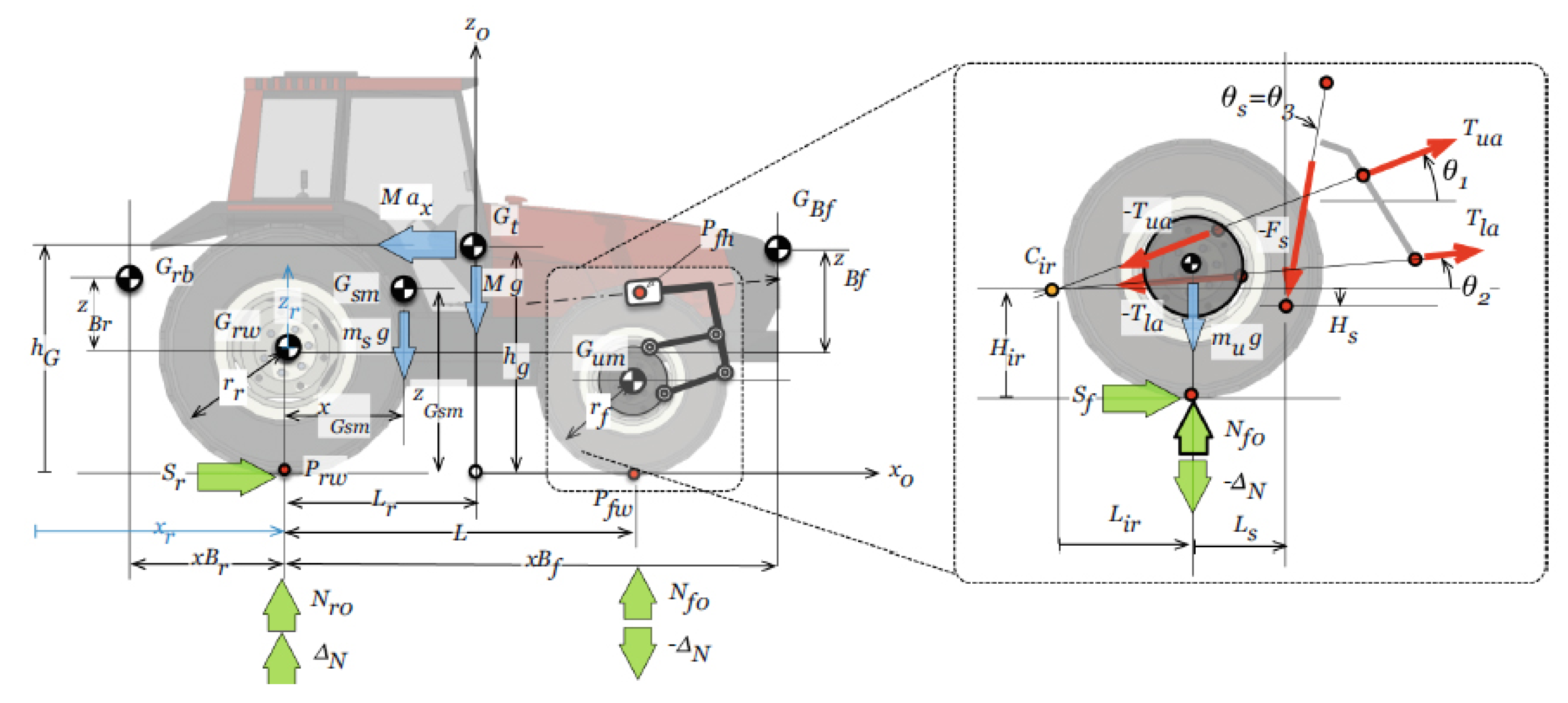
3.1.2. Dynamic Model
3.1.3. Mathematical Modeling
3.2. Logic and Control Systems
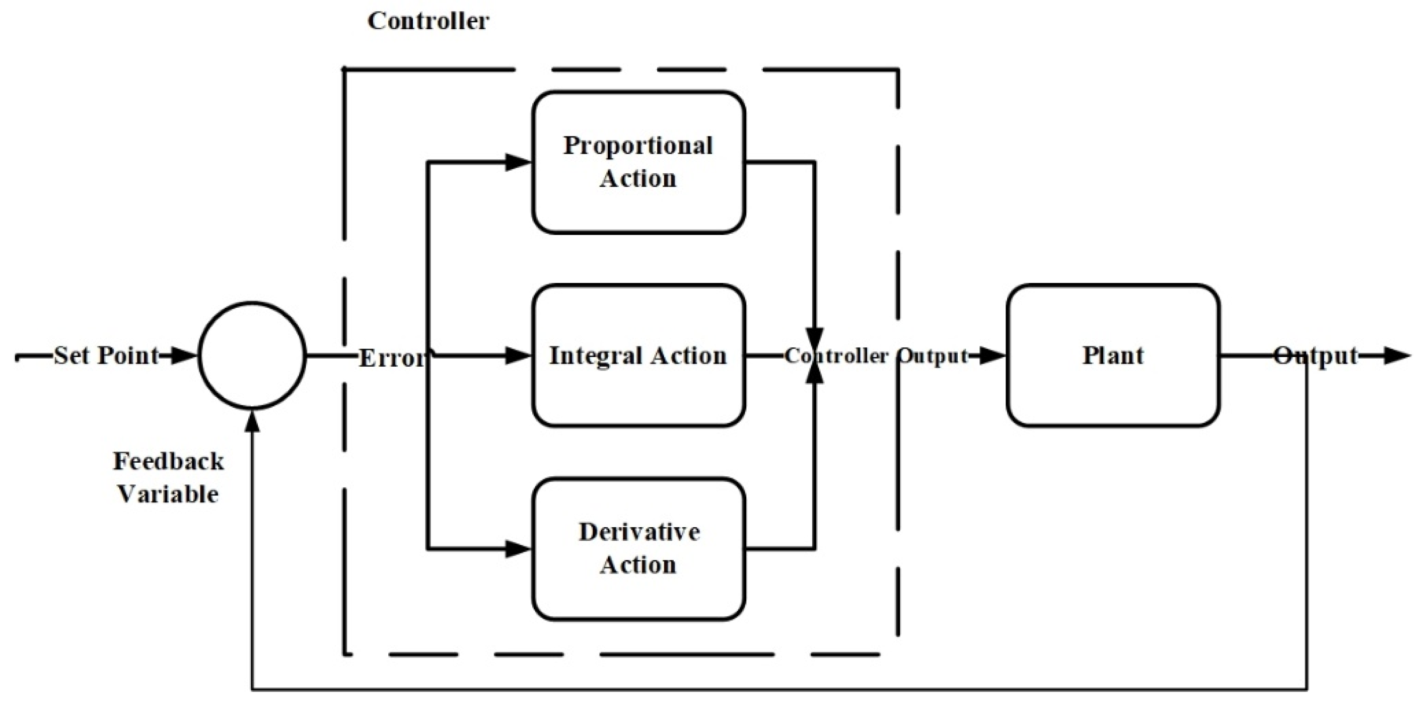
3.2.1. PID
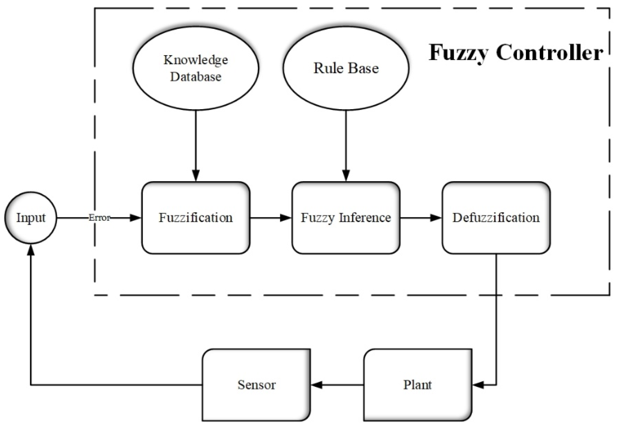
3.2.2. Fuzzy Logic
3.2.3. Genetic (Evolutionary) Algorithms
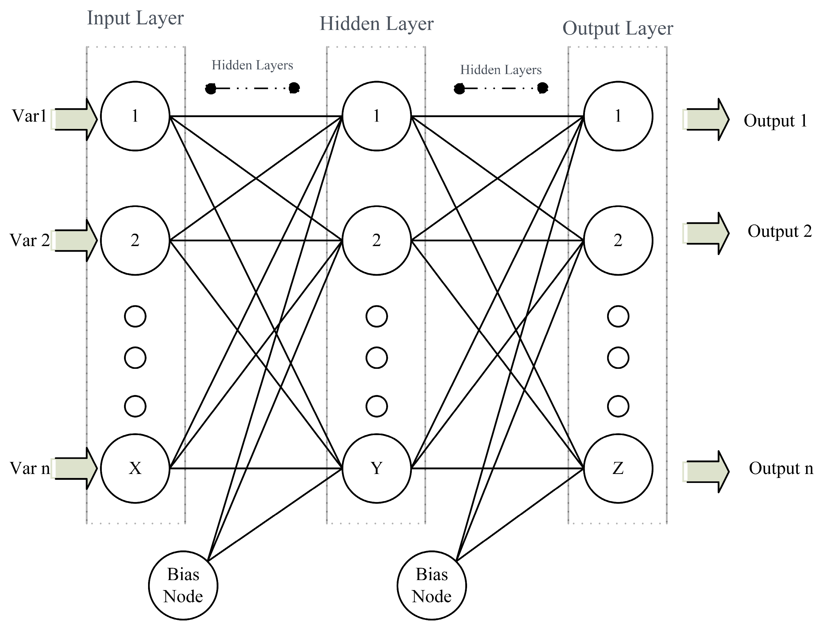
3.2.4. Artificial Neural Network
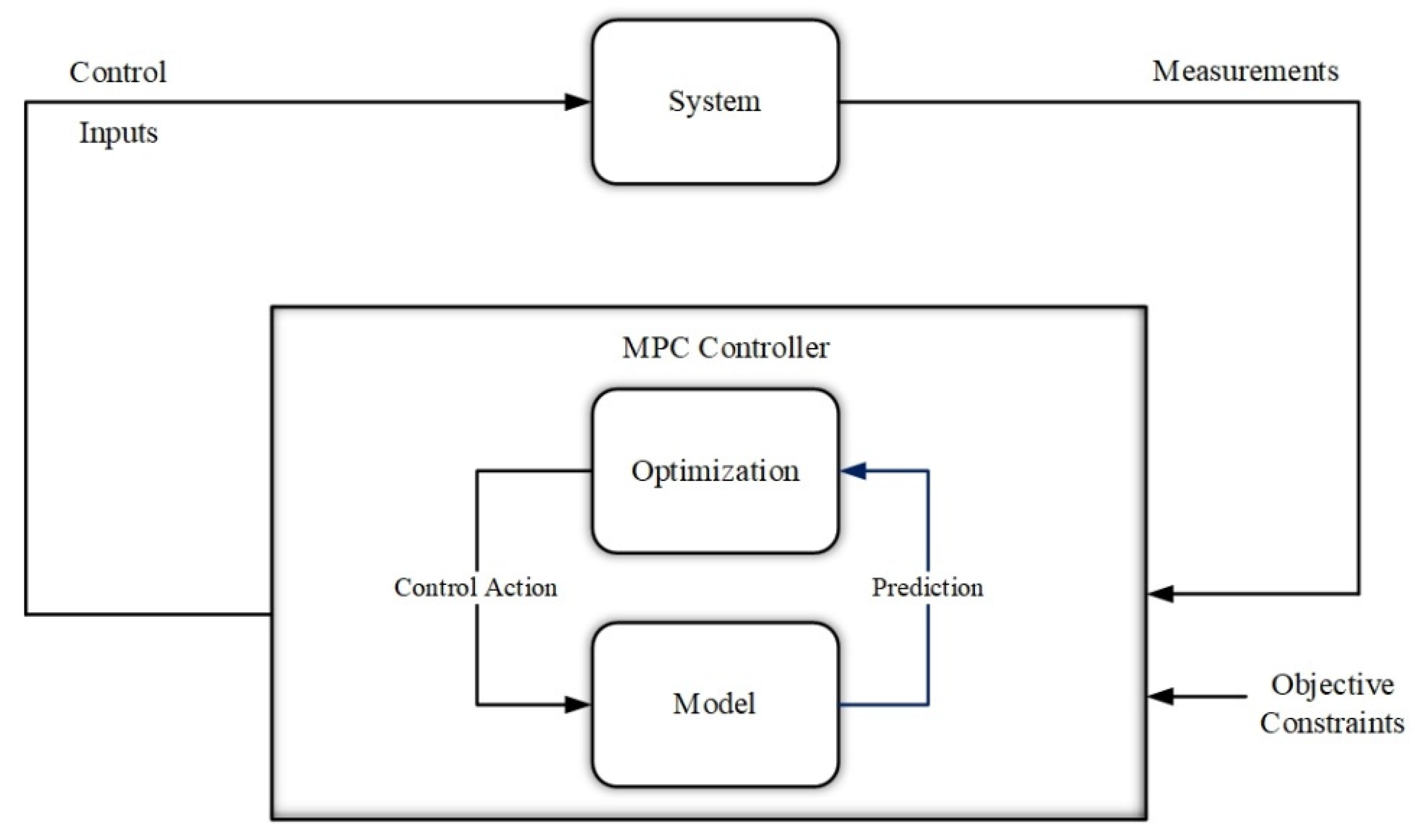
3.2.5. MPC
3.2.6. Kalman Filter
3.2.7. Machine Learning: DRL
4. Sensors
4.1. Attitude
4.2. Navigation Planners
4.3. Tracking Methods
4.4. Sensor Types
4.4.1. Vision
Computational Methods
Hough Transform
Kalman Filter
4.4.2. Position
GPS
Dead-Reckoning Sensors
4.4.3. Laser Sensors
4.4.4. Ultrasonic Sensor
4.4.5. Light Sensor (LiDAR)
4.4.6. Radar Sensor
4.4.7. Inertia Sensor
4.4.8. Geo-Magnetic Sensor
4.4.9. Safety Sensor
4.4.10. Power Status Sensors
Energy
4.4.11. Sensor Fusion
5. Data Communication
5.1. Types of Communications
5.1.1. Internal Communication
CAN
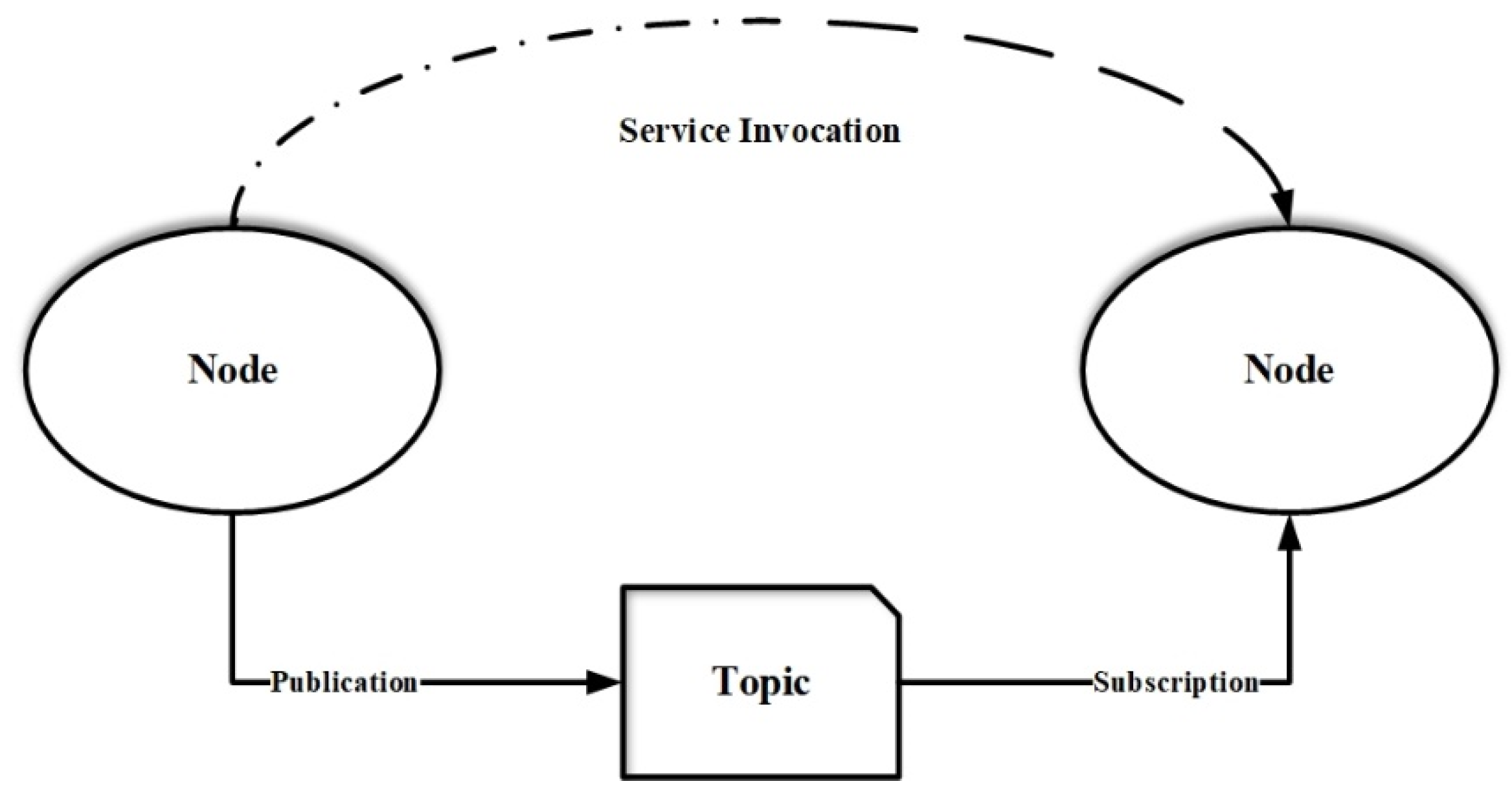
ROS
5.1.2. External Communication
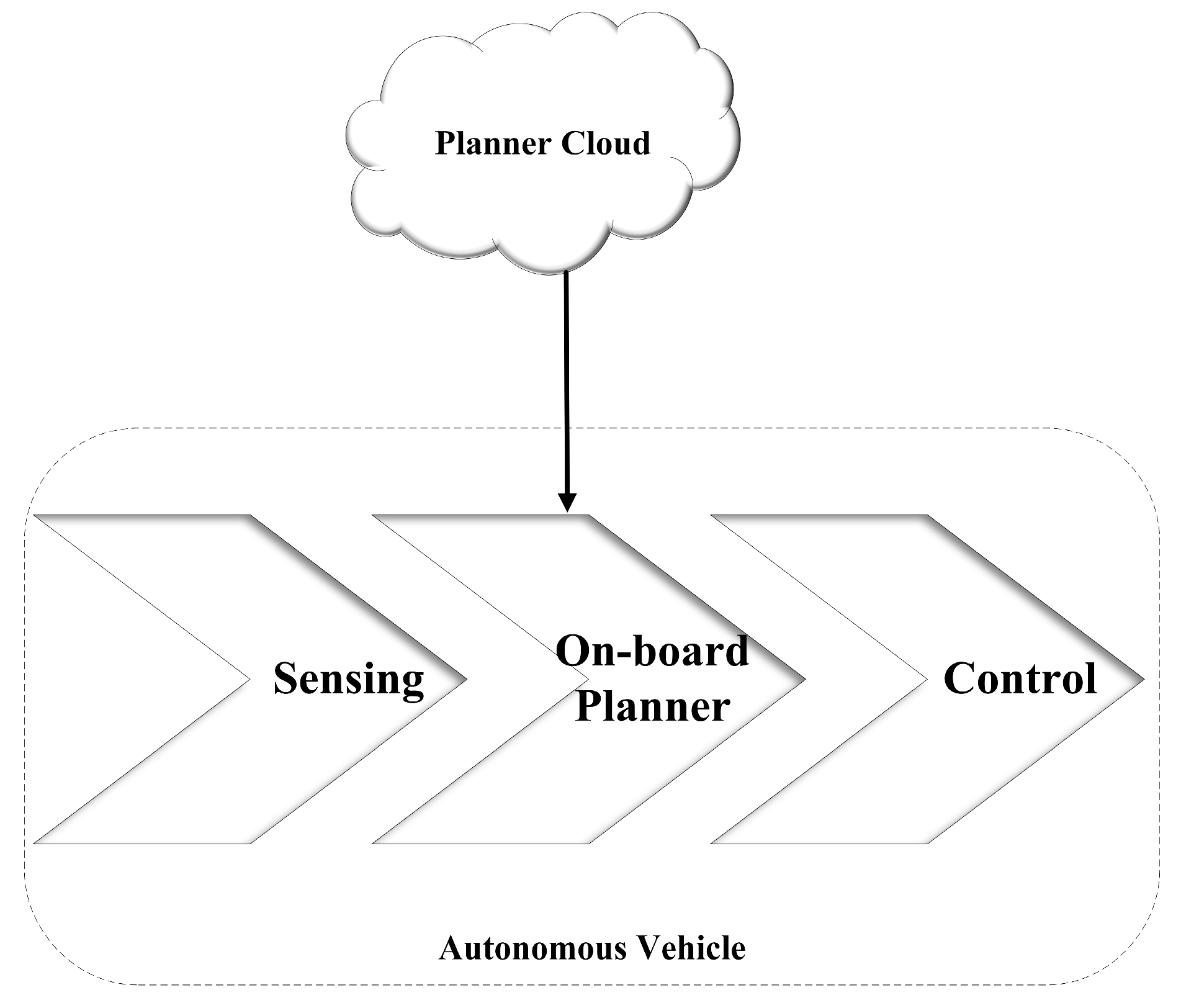
Cloud
6. Control Units and Actuators
6.1. Control Units
6.2. Actuators
6.2.1. Steering
6.2.2. Speed Control
6.2.3. Brake Control
6.3. Operation Control Consistency
7. Conclusions
Author Contributions
Funding
Informed Consent Statement
Data Availability Statement
Conflicts of Interest
References
- GMI. Global Market Insights. 2021. Available online: https://www.gminsights.com/industry-analysis/autonomous-farm-equipment-market (accessed on 13 March 2023).
- Singer, C.R. Agricultural Worker Shortage Could Rise to 114,000. 2021. Available online: https://www.immigration.ca/agricultural-worker-shortage-rise-114000/?nowprocket=1 (accessed on 13 March 2023).
- Future of Farming: Driverless Tractors, ag Robots. 2016. Available online: https://www.cnbc.com/2016/09/16/future-of-farming-driverless-tractors-ag-robots.html (accessed on 13 March 2023).
- McBain-Rigg, K.E.; Franklin, R.C.; McDonald, G.C.; Knight, S.M. Why Quad Bike Safety is a Wicked Problem: An Exploratory Study of Attitudes, Perceptions, and Occupational Use of Quad Bikes in Northern Queensland, Australia. J. Agric. Saf. Health 2014, 20, 33–50. [Google Scholar] [CrossRef] [PubMed]
- Patel, D.; Gandhi, M.; Shankaranarayanan, H.; Darji, A.D. Design of an Autonomous Agriculture Robot for Real-Time Weed Detection Using CNN. In Advances in VLSI and Embedded Systems; Lecture Notes in Electrical Engineering; Darji, A.D., Joshi, D., Joshi, A., Sheriff, R., Eds.; Springer: Singapore, 2023; Volume 962. [Google Scholar] [CrossRef]
- Bochtis, D.D.; Sørensen, C.G.; Busato, P. Advances in agricultural machinery management: A review. Biosyst. Eng. 2014, 126, 69–81. [Google Scholar] [CrossRef]
- Ayers, P.; Conger, J.B.; Comer, R.; Troutt, P. Stability Analysis of Agricultural Off-Road Vehicles. J. Agric. Saf. Health 2018, 24, 167–182. [Google Scholar] [CrossRef] [PubMed]
- Mcintosh, A.S.; Patton, D.A.; Rechnitzer, G.; Grzebieta, R. Injury mechanisms in fatal Australian quad bike incidents. Traffic Inj. Prev. 2016, 17, 386–390. [Google Scholar] [CrossRef] [PubMed]
- Abid, A.; Khan, M.T.; Iqbal, J. A review on fault detection and diagnosis techniques: Basics and beyond. Artif. Intell. Rev. 2021, 54, 3639–3664. [Google Scholar] [CrossRef]
- Gültekin, Ö.; Cinar, E.; Özkan, K.; Yazıcı, A. Multisensory data fusion-based deep learning approach for fault diagnosis of an industrial autonomous transfer vehicle. Expert Syst. Appl. 2022, 200, 117055. [Google Scholar] [CrossRef]
- Zellner, J.; Kebschull, S. Full-Scale Dynamic Overturn Tests of an ATV with and without a “Quadbar” CPD Using an Injury-Monitoring Dummy; Dynamic Research Inc.: Torrance, CA, USA, 2015. [Google Scholar]
- Kanchwala, H.; Chatterjee, A. ADAMS model validation for an all-terrain vehicle using test track data. Adv. Mech. Eng. 2019, 11. [Google Scholar] [CrossRef]
- Aras, M.; Zambri, M.; Azis, F.; Rashid, M.; Kamarudin, M. System identification modelling based on modification of all terrain vehicle (ATV) using wireless control system. J. Mech. Eng. Sci. 2015, 9, 1640–1654. [Google Scholar] [CrossRef]
- Petterson, T.C.; Gooch, S.D. Rolling Resistance of Atv Tyres In Agriculture. In Proceedings of the Design Society: DESIGN Conference, Cavtat, Croatia, 26–29 October 2020; Cambridge University Press: Cambridge, UK, 2020. [Google Scholar] [CrossRef]
- Board, T.R. Tires and Passenger Vehicle Fuel Economy: Informing Consumers, Improving Performance; Special Report 286; The National Academies Press: Washington, DC, USA, 2006; p. 174. [Google Scholar]
- Taheri, S.; Sandu, C.; Pinto, E.; Gorsich, D. A technical survey on Terramechanics models for tire–terrain interaction used in modeling and simulation of wheeled vehicles. J. Terramech. 2015, 57, 1–22. [Google Scholar] [CrossRef]
- Gallina, A.; Krenn, R.; Scharringhausen, M.; Uhl, T.; Schäfer, B. Parameter Identification of a Planetary Rover Wheel-Soil Contact Model via a Bayesian Approach. J. Field Robot. 2014, 31, 161–175. [Google Scholar] [CrossRef]
- Guo, T. Power Consumption Models for Tracked and Wheeled Small Unmanned Ground Vehicles on Deformable Terrains. Ph.D. Thesis, University of Michigan, Detroid, MI, USA, 2016. Available online: https://deepblue.lib.umich.edu/bitstream/handle/2027.42/133484/tianyou_1.pdf?sequence=1 (accessed on 13 March 2023).
- Dallas, J.; Jain, K.; Dong, Z.; Sapronov, L.; Cole, M.P.; Jayakumar, P.; Ersal, T. Online terrain estimation for autonomous vehicles on deformable terrains. J. Terramech. 2020, 91, 11–22. [Google Scholar] [CrossRef]
- Dallas, J.; Cole, P.M.; Jayakumar, P.; Ersal, T. Neural network based terramechanics modeling and estimation for deformable terrains. arXiv 2020, arXiv:2003.02635. [Google Scholar] [CrossRef]
- Shin, J.; Kwak, D.; Lee, T. Robust path control for an autonomous ground vehicle in rough terrain. Control Eng. Pract. 2020, 98, 104384. [Google Scholar] [CrossRef]
- Sock, J.; Kim, J.; Min, J.; Kwak, K. Probabilistic traversability map generation using 3D-LIDAR and camera. In Proceedings of the IEEE International Conference on Robotics and Automation (ICRA), Stockholm, Sweden, 16–21 May 2016; pp. 5631–5637. [Google Scholar]
- Mousazadeh, H. A technical review on navigation systems of agricultural autonomous off-road vehicles. J. Terramech. 2013, 50, 211–232. [Google Scholar] [CrossRef]
- Zhou, C.; Gu, S.; Wen, Y.; Du, Z.; Xiao, C.; Huang, L.; Zhu, M. The review unmanned surface vehicle path planning: Based on multi-modality constraint. Ocean Eng. 2020, 200, 107043. [Google Scholar] [CrossRef]
- Rus, C.; Leba, M.; Negru, N.; Marcuş, R.; Costandoiu, A. Autonomous Control System for an Electric ATV. MATEC Web Conf. 2021, 343, 6003. [Google Scholar] [CrossRef]
- Ma, X.; Hu, X.; Schweig, S.; Pragalathan, J.; Schramm, D. A Vehicle Guidance Model with a Close-to-Reality Driver Model and Different Levels of Vehicle Automation. Appl. Sci. 2021, 11, 380. [Google Scholar] [CrossRef]
- SAE J3016. 2019. Available online: https://www.sae.org/news/2019/01/sae-updates-j3016-automated-driving-graphic (accessed on 1 March 2023).
- Bak, T.; Jakobsen, H. Agricultural Robotic Platform with Four Wheel Steering for Weed Detection. Biosyst. Eng. 2004, 87, 125–136. [Google Scholar] [CrossRef]
- Li, M.; Imou, K.; Wakabayashi, K.; Yokoyama, S. Review of research on agricultural vehicle autonomous guidance. Int. J. Agric. Biol. Eng. 2009, 2, 1–16. [Google Scholar] [CrossRef]
- Heydinger, G.; Bixel, R.; Yapp, J.; Zagorski, S.; Sidhu, A.; Nowjack, J.; Jebode, H. Vehicle Characteristics Measurements of All-Terrain Vehicles; For Consumer Products Safety Commission Contract HHSP I; SEA Vehicle Dynamics Division: Columbus, OH, USA, 2016. [Google Scholar]
- Finch, H.J.S.; Samuel, A.M.; Lane, G.P.F. Introduction, in Lockhart & Wiseman’s Crop Husbandry Including Grassland, 9th ed.; Finch, H.J.S., Samuel, A.M., Lane, G.P.F., Eds.; Woodhead Publishing: Sawston, UK, 2014; pp. 17–42. [Google Scholar]
- Chou, H.-Y.; Khorsandi, F.; Vougioukas, S.G. Developing and Testing a GPS-Based Steering Control System for an Autonomous All-Terrain Vehicle. In Proceedings of the ASABE Annual International, Virtual, 13–15 July 2020; p. 1. [Google Scholar]
- Cheein, F.A.A.; Carelli, R. Agricultural Robotics: Unmanned Robotic Service Units in Agricultural Tasks. IEEE Ind. Electron. Mag. 2013, 7, 48–58. [Google Scholar] [CrossRef]
- Mavridou, E.; Vrochidou, E.; Papakostas, G.A.; Pachidis, T.; Kaburlasos, V.G. Machine Vision Systems in Precision Agriculture for Crop Farming. J. Imaging 2019, 5, 89. [Google Scholar] [CrossRef] [PubMed]
- Oliveira, L.F.P.; Moreira, A.P.; Silva, M.F. Advances in Agriculture Robotics: A State-of-the-Art Review and Challenges Ahead. Robotics 2021, 10, 52. [Google Scholar] [CrossRef]
- Chowdhury, M.Z.; Shahjalal, M.; Hasan, M.K.; Jang, Y.M. The Role of Optical Wireless Communication Technologies in 5G/6G and IoT Solutions: Prospects, Directions, and Challenges. Appl. Sci. 2019, 9, 4367. [Google Scholar] [CrossRef]
- Tomaszewski, L.; Kołakowski, R.; Zagórda, M. Application of mobile networks (5G and beyond) in precision agriculture. In Proceedings of the IFIP International Conference on Artificial Intelligence Applications and Innovations, Hersonissos, Greece, 17–20 June 2022; Springer: Berlin/Heidelberg, Germany, 2022. [Google Scholar] [CrossRef]
- Vougioukas, S.G. Agricultural robotics. Annual review of control, robotics, and autonomous systems. Ann. Rev. 2019, 2, 365–392. [Google Scholar]
- Roshanianfard, A.; Noguchi, N.; Okamoto, H.; Ishii, K. A review of autonomous agricultural vehicles (The experience of Hokkaido University). J. Terramech. 2020, 91, 155–183. [Google Scholar] [CrossRef]
- Goulet, N.; Ayalew, B. Energy-Optimal Ground Vehicle Trajectory Planning on Deformable Terrains. IFAC-PapersOnLine 2022, 55, 196–201. [Google Scholar] [CrossRef]
- Vantsevich, V.V.; Gorsich, D.J.; Paldan, J.R.; Ghasemi, M.; Moradi, L. Terrain mobility performance optimization: Fundamentals for autonomous vehicle applications. Part I. New mobility indices: Optimization and analysis. J. Terramech. 2022, 104, 31–47. [Google Scholar] [CrossRef]
- Jonsson, F. CAKE-Kibb. 2022. Available online: https://www.umu.se/en/umea-institute-of-design/education/student-work/masters-programme-in-transportation-design/2022/fanny-jonsson/ (accessed on 3 March 2023).
- Erian, K.H. Autonomous Control of an All-Terrain Vehicle Using Embedded Systems and Artificial Intelligence Techniques. Ph.D. Thesis, The University of North Carolina at Charlotte, Charlotte, NC, USA, 2022. ACM Digital Library. Available online: https://dl.acm.org/doi/book/10.5555/AAI29164332 (accessed on 13 March 2023).
- Reid, J.F.; Zhang, Q.; Noguchi, N.; Dickson, M. Agricultural automatic guidance research in North America. Comput. Electron. Agric. 2000, 25, 155–167. [Google Scholar] [CrossRef]
- Tillett, N. Automatic guidance sensors for agricultural field machines: A review. J. Agric. Eng. Res. 1991, 50, 167–187. [Google Scholar] [CrossRef]
- Murakami, N.; Ito, A.; Will, J.D.; Steffen, M.; Inoue, K.; Kita, K.; Miyaura, S. Environment identification technique using hyper omni-vision and image map. In Proceedings of the 3rd IFAC International Workshop Bio-Robotics, Sapporo, Japan, 6–8 September 2006. [Google Scholar]
- Klančar, G.; Zdešar, A.; Blažič, S.; Škrjanc, I. Chapter 2—Motion Modeling for Mobile Robots. In Wheeled Mobile Robotics; Klančar, G., Zdešar, A., Blažič, S., Škrjanc, I., Eds.; Butterworth-Heinemann: Oxford, UK, 2017; pp. 13–59. [Google Scholar]
- Kayacan, E.; Kayacan, E.; Ramon, H.; Saeys, W. Towards agrobots: Identification of the yaw dynamics and trajectory tracking of an autonomous tractor. Comput. Electron. Agric. 2015, 115, 78–87. [Google Scholar] [CrossRef]
- Benson, E.; Stombaugh, T.S.; Noguchi, N.; Will, J.D.; Reid, J.F. An evaluation of a geomagnetic direction sensor for vehicle guidance in precision agriculture applications. In Proceedings of the ASAE Annual International Meeting, Orlando, FL, USA, 12–15 July 1998. [Google Scholar]
- O’Connor, M.; Bell, T.; Elkaim, G.; Parkinson, B. Automatic steering of farm vehicles using GPS. In Proceedings of the 3rd International Conference on Precision Agriculture, Minneapolis, MN, USA, 23–26 June 1996; Wiley and Sons: Hoboken, NJ, USA, 1996. [Google Scholar] [CrossRef]
- Zhang, Q.; Wu, D.; Reid, J.; Benson, E. Model recognition and validation for an off-road vehicle electrohydraulic steering controller. Mechatronics 2002, 12, 845–858. [Google Scholar] [CrossRef]
- Fang, H.; Fan, R.; Thuilot, B.; Martinet, P. Trajectory tracking control of farm vehicles in presence of sliding. Robot. Auton. Syst. 2006, 54, 828–839. [Google Scholar] [CrossRef]
- Lenain, R.; Thuilot, B.; Cariou, C.; Martinet, P. Model Predictive Control for Vehicle Guidance in Presence of Sliding: Application to Farm Vehicles Path Tracking. In Proceedings of the IEEE International Conference on Robotics and Automation, Barcelona, Spain, 18–22 April 2005; pp. 885–890. [Google Scholar]
- Lenain, R.; Thuilot, B.; Cariou, C.; Martinet, P. High accuracy path tracking for vehicles in presence of sliding: Application to farm vehicle automatic guidance for agricultural tasks. Auton. Robot. 2006, 21, 79–97. [Google Scholar] [CrossRef]
- Franceschetti, B.; Lenain, R.; Rondelli, V. Comparison between a rollover tractor dynamic model and actual lateral tests. Biosyst. Eng. 2014, 127, 79–91. [Google Scholar] [CrossRef]
- Kayacan, E.; Kayacan, E.; Ramon, H.; Saeys, W. Learning in Centralized Nonlinear Model Predictive Control: Application to an Autonomous Tractor-Trailer System. IEEE Trans. Control Syst. Technol. 2014, 23, 197–205. [Google Scholar] [CrossRef]
- Bouton, N.; Lenain, R.; Thuilot, B.; Martinet, P. Backstepping observer dedicated to tire cornering stiffness estimation: Application to an all terrain vehicle and a farm tractor. In Proceedings of the IEEE/RSJ International Conference on Intelligent Robots and Systems, San Diego, CA, USA, 29 October–2 November 2007; pp. 1763–1768. [Google Scholar]
- Biral, F.; Pelanda, R.; Cis, A. Anti-dive front suspension for agricultural tractors: Dynamic model and validation. In Advances in Italian Mechanism Science: Proceedings of the First International Conference of IFToMM Italy; Springer: Berlin/Heidelberg, Germany, 2017. [Google Scholar] [CrossRef]
- Pan, K.; Zheng, W.; Shen, X. Optimization Design and Analysis of All-terrain Vehicle Based on Modal Analysis. J. Phys. Conf. Ser. 2021, 1885, 52055. [Google Scholar] [CrossRef]
- Alipour, K.; Robat, A.B.; Tarvirdizadeh, B. Dynamics modeling and sliding mode control of tractor-trailer wheeled mobile robots subject to wheels slip. Mech. Mach. Theory 2019, 138, 16–37. [Google Scholar] [CrossRef]
- Liao, J.; Chen, Z.; Yao, B. Model-Based Coordinated Control of Four-Wheel Independently Driven Skid Steer Mobile Robot with Wheel–Ground Interaction and Wheel Dynamics. IEEE Trans. Ind. Inform. 2018, 15, 1742–1752. [Google Scholar] [CrossRef]
- Fnadi, M.; Plumet, F.; Amar, F.B. Nonlinear Tire Cornering Stiffness Observer for a Double Steering Off-Road Mobile Robot. In Proceedings of the 2019 International Conference on Robotics and Automation (ICRA), Montreal, QC, Canada, 24 May 2019; pp. 7529–7534. [Google Scholar] [CrossRef]
- Feng, L.; He, Y.; Bao, Y.; Fang, H. Development of Trajectory Model for a Tractor-Implement System for Automated Navigation Applications. In Proceedings of the IEEE Instrumentation and Measurement Technology, Ottawa, ON, Canada, 16–19 May 2005; pp. 1330–1334. [Google Scholar]
- Soe, T.T.; Tun, H.M. Implementation of Double Closed-Loop Control System for Unmanned Ground Vehicles. Int. J. Sci. Technol. Res. 2014, 3, 257–262. [Google Scholar]
- Kim, J.-H.; Kim, C.-K.; Jo, G.-H.; Kim, B.-W. The research of parking mission planning algorithm for unmanned ground vehicle. In Proceedings of the 2010 International Conference on Control, Automation and Systems (ICCAS 2010), Gyeonggi-do, Republic of Korea, 27–30 October 2010; pp. 1093–1096. [Google Scholar] [CrossRef]
- Deur, J.; Petric, J.; Asgari, J.; Hrovat, D. Recent Advances in Control-Oriented Modeling of Automotive Power Train Dynamics. In Proceedings of the IEEE International Symposium on Industrial Electronics, Dubrovnik, Croatia, 20–23 June 2005; pp. 269–278. [Google Scholar] [CrossRef]
- Tran, T.H.; Kwok, N.M.; Scheding, S.; Ha, Q.P. Dynamic Modelling of Wheel-Terrain Interaction of a UGV. In Proceedings of the 2007 IEEE International Conference on Automation Science and Engineering, Scottsdale, AZ, USA, 22–25 September 2007; pp. 369–374. [Google Scholar] [CrossRef]
- Dave, P.N.; Patil, J.B. Modeling and control of nonlinear unmanned ground all terrain vehicle. In Proceedings of the 2015 International Conference on Trends in Automation, Communications and Computing Technology (I-TACT-15), Bangalore, India, 21–22 December 2015; pp. 1–7. [Google Scholar] [CrossRef]
- Cho, S.I.; Lee, J.H. Autonomous Speedsprayer using Differential Global Positioning System, Genetic Algorithm and Fuzzy Control. J. Agric. Eng. Res. 2000, 76, 111–119. [Google Scholar] [CrossRef]
- Kodagoda, K.R.S.; Wijesoma, W.S.; Teoh, E.K. Fuzzy speed and steering control of an AGV. IEEE Trans. Control Syst. Technol. 2002, 10, 112–120. [Google Scholar] [CrossRef]
- Cortner, A.; Conrad, J.M.; BouSaba, N.A. Autonomous all-terrain vehicle steering. In Proceedings of the IEEE Southeastcon, Orlando, FL, USA, 15–18 March 2012; pp. 1–5. [Google Scholar] [CrossRef]
- Eski, I.; Kuş, Z.A. Control of unmanned agricultural vehicles using neural network-based control system. Neural Comput. Appl. 2019, 31, 583–595. [Google Scholar] [CrossRef]
- Hossain, T.; Habibullah, H.; Islam, R. Steering and Speed Control System Design for Autonomous Vehicles by Developing an Optimal Hybrid Controller to Track Reference Trajectory. Machines 2022, 10, 420. [Google Scholar] [CrossRef]
- Behrooz, F.; Mariun, N.; Marhaban, M.H.; Radzi, M.A.M.; Ramli, A.R. Review of Control Techniques for HVAC Systems—Nonlinearity Approaches Based on Fuzzy Cognitive Maps. Energies 2018, 11, 495. [Google Scholar] [CrossRef]
- Sumarsono, S. Control System for an All Terrain Vehicle Using DGPS and Fuzzy Logic, in Civil and Environmental Engineering. Ph.D. Thesis, University of Melbourne, Melbourne, Australia, 1999. [Google Scholar]
- Delavarpour, N.; Eshkabilov, S.; Bon, T.; Nowatzki, J.; Bajwa, S. The Tractor-Cart System Controller with Fuzzy Logic Rules. Appl. Sci. 2020, 10, 5223. [Google Scholar] [CrossRef]
- Bonadies, S.; Smith, N.; Niewoehner, N.; Lee, A.S.; Lefcourt, A.M.; Gadsden, S.A. Development of Proportional–Integral–Derivative and Fuzzy Control Strategies for Navigation in Agricultural Environments. J. Dyn. Syst. Meas. Control 2018, 140, 4038504. [Google Scholar] [CrossRef]
- Yao, L.; Pitla, S.K.; Zhao, C.; Liew, C.; Hu, D.; Yang, Z. An Improved Fuzzy Logic Control Method for Path Tracking of an Autonomous Vehicle. Trans. ASABE 2020, 63, 1895–1904. [Google Scholar] [CrossRef]
- Fleming, P.; Purshouse, R. Evolutionary algorithms in control systems engineering: A survey. Control Eng. Pract. 2002, 10, 1223–1241. [Google Scholar] [CrossRef]
- Mathworks. Available online: https://www.mathworks.com/help/gads/what-is-the-genetic-algorithm.html (accessed on 21 March 2023).
- Ryerson, A.F.; Zhang, Q. Vehicle path planning for complete field coverage using genetic algorithms. Agric. Eng. Int. CIGR J. 2007, IX. [Google Scholar]
- Ashraf, M.A.; Takeda, J.-I.; Torisu, R. Neural Network Based Steering Controller for Vehicle Navigation on Sloping Land. Eng. Agric. Environ. Food 2010, 3, 100–104. [Google Scholar] [CrossRef]
- Shiltagh, N.A.; Jalal, L.D. Path planning of intelligent mobile robot using modified genetic algorithm. Int. J. Soft Comput. Eng. 2013, 3, 31–36. [Google Scholar]
- Chen, Z.; Xiao, J.; Wang, G. An Effective Path Planning of Intelligent Mobile Robot Using Improved Genetic Algorithm. Wirel. Commun. Mob. Comput. 2022, 2022, 9590367. [Google Scholar] [CrossRef]
- Torisu, R.; Hai, S.; Takeda, J.-I.; Ashraf, M.A. Automatic Tractor Guidance on Sloped Terrain (Part 1) Formulation of NN Vehicle Model and Design of control Law for contour Line Travel. J. Jpn. Soc. Agric. Mach. 2002, 64, 88–95. [Google Scholar] [CrossRef]
- Kamilaris, A.; Prenafeta-Boldú, F.X. Deep learning in agriculture: A survey. Comput. Electron. Agric. 2018, 147, 70–90. [Google Scholar] [CrossRef]
- Afram, A.; Janabi-Sharifi, F. Theory and Applications of HVAC Control systems–A Review of Model Predictive Control (MPC). Build. Environ. 2014, 72, 343–355. [Google Scholar] [CrossRef]
- Christofides, P.D.; Scattolini, R.; de la Peña, D.M.; Liu, J. Distributed model predictive control: A tutorial review and future research directions. Comput. Chem. Eng. 2013, 51, 21–41. [Google Scholar] [CrossRef]
- Wang, Y.-G.; Shi, Z.-G.; Cai, W.-J. PID autotuner and its application in HVAC systems. In Proceedings of the American Control Conference, Arlington, VA, USA, 25–27 June 2001; Volume 3, pp. 2192–2196. [Google Scholar] [CrossRef]
- Froisy, J.B. Model predictive control: Past, present and future. ISA Trans. 1994, 33, 235–243. [Google Scholar] [CrossRef]
- Morari, M.; Lee, J.H. Model predictive control: Past, present and future. Comput. Chem. Eng. 1999, 23, 667–682. [Google Scholar] [CrossRef]
- Qin, S.; Badgwell, T.A. A survey of industrial model predictive control technology. Control Eng. Pract. 2003, 11, 733–764. [Google Scholar] [CrossRef]
- Rawlings, J.B.; Mayne, D.Q. Model Predictive Control: Theory and Design, 2nd ed.; Nob Hill Pub LLC: San Francisco, CA, USA, 2009. [Google Scholar]
- Han, H.; Qiao, J. Nonlinear Model-Predictive Control for Industrial Processes: An Application to Wastewater Treatment Process. IEEE Trans. Ind. Electron. 2013, 61, 1970–1982. [Google Scholar] [CrossRef]
- Lu, E.; Xue, J.; Chen, T.; Jiang, S. Robust Trajectory Tracking Control of an Autonomous Tractor-Trailer Considering Model Parameter Uncertainties and Disturbances. Agriculture 2023, 13, 869. [Google Scholar] [CrossRef]
- Coen, T.; Anthonis, J.; De Baerdemaeker, J. Cruise control using model predictive control with constraints. Comput. Electron. Agric. 2008, 63, 227–236. [Google Scholar] [CrossRef]
- Backman, J.; Oksanen, T.; Visala, A. Navigation system for agricultural machines: Nonlinear Model Predictive path tracking. Comput. Electron. Agric. 2012, 82, 32–43. [Google Scholar] [CrossRef]
- Horvath, K.; Petreczky, M.; Rajaoarisoa, L.; Duviella, E.; Chuquet, K. MPC control of water level in a navigation canal—The Cuinchy-Fontinettes case study. In Proceedings of the 2014 European Control Conference (ECC), Strasbourg, France, 24–27 June 2014; pp. 1337–1342. [Google Scholar] [CrossRef]
- Kayacan, E.; Kayacan, E.; Ramon, H.; Saeys, W. Distributed nonlinear model predictive control of an autonomous tractor–trailer system. Mechatronics 2014, 24, 926–933. [Google Scholar] [CrossRef]
- Bin, Y.; Shim, T. Constrained model predictive control for backing-up tractor-trailer system. In Proceedings of the 10th World Congress on Intelligent Control and Automation (WCICA 2012), Beijing, China, 6–8 July 2012; pp. 2165–2170. [Google Scholar] [CrossRef]
- Yakub, F.; Mori, Y. Comparative study of autonomous path-following vehicle control via model predictive control and linear quadratic control. Proc. Inst. Mech. Eng. Part D J. Automob. Eng. 2015, 229, 1695–1714. [Google Scholar] [CrossRef]
- Plessen, M.M.G.; Bemporad, A. Reference trajectory planning under constraints and path tracking using linear time-varying model predictive control for agricultural machines. Biosyst. Eng. 2017, 153, 28–41. [Google Scholar] [CrossRef]
- Kalmari, J.; Backman, J.; Visala, A. Nonlinear model predictive control of hydraulic forestry crane with automatic sway damping. Comput. Electron. Agric. 2014, 109, 36–45. [Google Scholar] [CrossRef]
- Kalmari, J.; Backman, J.; Visala, A. Coordinated motion of a hydraulic forestry crane and a vehicle using nonlinear model predictive control. Comput. Electron. Agric. 2017, 133, 119–127. [Google Scholar] [CrossRef]
- Ding, Y.; Wang, L.; Li, Y.; Li, D. Model predictive control and its application in agriculture: A review. Comput. Electron. Agric. 2018, 151, 104–117. [Google Scholar] [CrossRef]
- Kalmanfilter. Available online: https://www.kalmanfilter.net/kalman1d.html (accessed on 1 April 2023).
- Gan-Mor, S.; Upchurch, B.; Clark, R.; Hardage, D. Implement Guidance Error as Affected by Field Conditions Using Automatic DGPS Tractor Guidance; American Society of Agricultural and Biological Engineers: St. Joseph, MI, USA, 2002. [Google Scholar]
- Shen, J.; Huang, X. GNSS Application Case Agricultural Auto-Steering and Guidance Systems. In Proceedings of the 16thMeeting of the International Committee on Global Navigation Satellite Systems (ICG-16), Abu Dhabi, United Arab Emirates, 10–14 October 2022; Beijing UniStrong Science and Technology Co., Ltd.: Beijing, China, 2022. Available online: https://www.unoosa.org (accessed on 1 April 2023).
- Nagasaka, Y.; Umeda, N.; Kanetai, Y.; Taniwaki, K.; Sasaki, Y. Autonomous guidance for rice transplanting using global positioning and gyroscopes. Comput. Electron. Agric. 2004, 43, 223–234. [Google Scholar] [CrossRef]
- Nørremark, M.; Griepentrog, H.; Nielsen, J.; Søgaard, H. The development and assessment of the accuracy of an autonomous GPS-based system for intra-row mechanical weed control in row crops. Biosyst. Eng. 2008, 101, 396–410. [Google Scholar] [CrossRef]
- Han, S.; Zhang, Q.; Ni, B.; Reid, J. A guidance directrix approach to vision-based vehicle guidance systems. Comput. Electron. Agric. 2004, 43, 179–195. [Google Scholar] [CrossRef]
- Hague, T.; Tillett, N. A bandpass filter-based approach to crop row location and tracking. Mechatronics 2001, 11, 1–12. [Google Scholar] [CrossRef]
- Crassidis, J.L. Sigma-point Kalman filtering for integrated GPS and inertial navigation. IEEE Trans. Aerosp. Electron. Syst. 2006, 42, 750–756. [Google Scholar] [CrossRef]
- Zhang, Y.; Gao, F.; Tian, L. INS/GPS integrated navigation for wheeled agricultural robot based on sigma-point Kalman Filter. In Proceedings of the 2008 Asia Simulation Conference–7th International Conference on System Simulation and Scientific Computing (ICSC), Beijing, China, 10–12 October 2008; pp. 1425–1431. [Google Scholar] [CrossRef]
- Pratama, P.S.; Gulakari, A.V.; Setiawan, Y.D.; Kim, D.H.; Kim, H.K.; Kim, S.B. Trajectory tracking and fault detection algorithm for automatic guided vehicle based on multiple positioning modules. Int. J. Control Autom. Syst. 2016, 14, 400–410. [Google Scholar] [CrossRef]
- Gao, B.; Hu, G.; Zhu, X.; Zhong, Y. A Robust Cubature Kalman Filter with Abnormal Observations Identification Using the Mahalanobis Distance Criterion for Vehicular INS/GNSS Integration. Sensors 2019, 19, 5149. [Google Scholar] [CrossRef] [PubMed]
- Lillicrap, T.P. Continuous control with deep reinforcement learning. arXiv 2015, arXiv:1509.02971. Available online: http://arxiv.org/abs/1509.02971 (accessed on 21 April 2023).
- Mnih, V.; Kavukcuoglu, K.; Silver, D.; Graves, A.; Antonoglou, I.; Wierstra, D.; Riedmiller, M. Playing atari with deep reinforcement learning. arXiv 2013, arXiv:1312.5602. [Google Scholar] [CrossRef]
- Josef, S.; Degani, A. Deep Reinforcement Learning for Safe Local Planning of a Ground Vehicle in Unknown Rough Terrain. IEEE Robot. Autom. Lett. 2020, 5, 6748–6755. [Google Scholar] [CrossRef]
- Kahn, G.; Villaflor, A.; Ding, B.; Abbeel, P.; Levine, S. Self-Supervised Deep Reinforcement Learning with Generalized Computation Graphs for Robot Navigation. In Proceedings of the 2018 IEEE International Conference on Robotics and Automation (ICRA), Brisbane, Australia, 21–25 May 2018; pp. 1–8. [Google Scholar] [CrossRef]
- Wiberg, V.; Wallin, E.; Nordfjell, T.; Servin, M. Control of Rough Terrain Vehicles Using Deep Reinforcement Learning. IEEE Robot. Autom. Lett. 2021, 7, 390–397. [Google Scholar] [CrossRef]
- Ampatzidis, Y.G.; Vougioukas, S.G.; Bochtis, D.D.; Tsatsarelis, C.A. A yield mapping system for hand-harvested fruits based on RFID and GPS location technologies: Field testing. Precis. Agric. 2009, 10, 63–72. [Google Scholar] [CrossRef]
- Narvaez, F.Y.; Reina, G.; Torres-Torriti, M.; Kantor, G.; Cheein, F.A. A Survey of Ranging and Imaging Techniques for Precision Agriculture Phenotyping. IEEE/ASME Trans. Mechatron. 2017, 22, 2428–2439. [Google Scholar] [CrossRef]
- Prado, J.; Michałek, M.M.; Cheein, F.A. Machine-learning based approaches for self-tuning trajectory tracking controllers under terrain changes in repetitive tasks. Eng. Appl. Artif. Intell. 2018, 67, 63–80. [Google Scholar] [CrossRef]
- Moshou, D.; Bravo, C.; Oberti, R.; West, J.S.; Ramon, H.; Vougioukas, S.; Bochtis, D. Intelligent multi-sensor system for the detection and treatment of fungal diseases in arable crops. Biosyst. Eng. 2011, 108, 311–321. [Google Scholar] [CrossRef]
- Rahnemoonfar, M.; Sheppard, C. Deep Count: Fruit Counting Based on Deep Simulated Learning. Sensors 2017, 17, 905. [Google Scholar] [CrossRef] [PubMed]
- Vasconez, J.P.; Salvo, J.; Auat, F. Toward Semantic Action Recognition for Avocado Harvesting Process based on Single Shot MultiBox Detector. In Proceedings of the 2018 IEEE International Conference on Automation/23rd Congress of the Chilean Association of Automatic Control (ICA-ACCA), Concepcion, Chile, 17–19 October 2018; pp. 1–6. [Google Scholar] [CrossRef]
- Xiong, L.; Xia, X.; Lu, Y.; Liu, W.; Gao, L.; Song, S.; Han, Y.; Yu, Z. IMU-Based Automated Vehicle Slip Angle and Attitude Estimation Aided by Vehicle Dynamics. Sensors 2019, 19, 1930. [Google Scholar] [CrossRef] [PubMed]
- Yang, Y.; Fu, M.; Zhu, H.; Xiong, G.; Sun, C. Control methods of mobile robot rough-terrain trajectory tracking. In Proceedings of the 8th IEEE International Conference on Control and Automation (ICCA 2010), Xiamen, China, 9–11 June 2010; pp. 731–738. [Google Scholar] [CrossRef]
- Ishii, K.; Terao, H.; Noguchi, N. Studies on Self-learning Autonomous Vehicles (Part 3) Positioning System for Autonomous Vehicle. J. Jpn. Soc. Agric. Mach. 1998, 60, 51–58. [Google Scholar]
- Benson, E.; Reid, J.; Zhang, Q. Machine Vision-based Guidance System for Agricultural Grain Harvesters using Cut-edge Detection. Biosyst. Eng. 2003, 86, 389–398. [Google Scholar] [CrossRef]
- Marchant, J.A.; Brivot, R. Real-Time Tracking of Plant Rows Using a Hough Transform. Real-Time Imaging 1995, 1, 363–371. [Google Scholar] [CrossRef]
- Søgaard, H.; Olsen, H. Determination of crop rows by image analysis without segmentation. Comput. Electron. Agric. 2003, 38, 141–158. [Google Scholar] [CrossRef]
- Okamoto, H.; Hamada, K.; Kataoka, T.; Hata, M.T.A.S.; Terawaki, M.; Hata, S. Automatic Guidance System with Crop Row Sensor. In Proceedings of the Automation Technology for Off-Road Equipment, Chicago, IL, USA, 26–27 July 2002; p. 307. [Google Scholar] [CrossRef]
- Billingsley, J.; Schoenfisch, M. The successful development of a vision guidance system for agriculture. Comput. Electron. Agric. 1997, 16, 147–163. [Google Scholar] [CrossRef]
- Kise, M.; Zhang, Q.; Más, F.R. A Stereovision-based Crop Row Detection Method for Tractor-automated Guidance. Biosyst. Eng. 2005, 90, 357–367. [Google Scholar] [CrossRef]
- Barawid, O.C.; Mizushima, A.; Ishii, K.; Noguchi, N. Development of an Autonomous Navigation System using a Two-dimensional Laser Scanner in an Orchard Application. Biosyst. Eng. 2007, 96, 139–149. [Google Scholar] [CrossRef]
- Lee, J.-W.; Choi, S.-U.; Lee, Y.-J.; Lee, K. A study on recognition of road lane and movement of vehicles using vision system. In Proceedings of the 40th SICE Annual Conference (SICE 2001), Nagoya, Japan, 27 July 2001; pp. 38–41. [Google Scholar] [CrossRef]
- Leemans, V.; Destain, M.-F. Line cluster detection using a variant of the Hough transform for culture row localisation. Image Vis. Comput. 2006, 24, 541–550. [Google Scholar] [CrossRef]
- Marchant, J. Tracking of row structure in three crops using image analysis. Comput. Electron. Agric. 1996, 15, 161–179. [Google Scholar] [CrossRef]
- Yu, B.; Jain, A. Lane boundary detection using a multiresolution Hough transform. In Proceedings of the International Conference on Image Processing, Santa Barbara, CA, USA, 26–29 October 1997; Volume 2, pp. 748–751. [Google Scholar] [CrossRef]
- Kalman, R.E. A New Approach to Linear Filtering and Prediction Problems. J. Basic Eng. 1960, 82, 35–45. [Google Scholar] [CrossRef]
- Heidman, B.; Abidine, A.; Upadhyaya, S.; Hills, D. Application of RTK GPS based auto-guidance system in agricultural production. In Proceedings of the 6th International Conference on Precision Agriculture and Other Precision Resources Management, Minneapolis, MN, USA, 14–17 July 2002; American Society of Agronomy: Minneapolis, MN, USA, 2003. [Google Scholar]
- Kumagai, H.; Kubo, Y.; Kihara, M.; Sugimoto, S. DGPS/INS/VMS Integration for High Accuracy Land-Vehicle Positioning. In Proceedings of the 12th International Technical Meeting of the Satellite Division of The Institute of Navigation (ION GPS 1999), Nashville, TN, USA, 14–17 September 1999. [Google Scholar] [CrossRef]
- Bell, T. Automatic tractor guidance using carrier-phase differential GPS. Comput. Electron. Agric. 2000, 25, 53–66. [Google Scholar] [CrossRef]
- Gan-Mor, S.; Ronen, B.; Josef, S.; Bilanki, Y. Guidance of Automatic Vehicle for Greenhouse Transportation. Acta Hortic. 1996, 1, 99–104. [Google Scholar] [CrossRef]
- Larsen, W.; Nielsen, G.; Tyler, D. Precision navigation with GPS. Comput. Electron. Agric. 1994, 11, 85–95. [Google Scholar] [CrossRef]
- Yamamoto, S.; Yukumoto, O.; Matsuo, Y. Robotization of Agricultural Vehicles—Various Operation with Tilling Robot. IFAC Proc. Vol. 2000, 34, 203–208. [Google Scholar] [CrossRef]
- Slaughter, D.; Giles, D.; Downey, D. Autonomous robotic weed control systems: A review. Comput. Electron. Agric. 2008, 61, 63–78. [Google Scholar] [CrossRef]
- Kise, M.; Noguchi, N.; Ishii, K.; Terao, H. Development of the Agricultural Autonomous Tractor with an RTK-GPS and a Fog. IFAC Proc. Vol. 2001, 34, 99–104. [Google Scholar] [CrossRef]
- Kise, M.; Noguchi, N.; Ishii, K.; Terao, H. The Development of the Autonomous Tractor with Steering Controller Applied by Optimal Control. In Proceedings of the Automation Technology for Off-Road Equipment, Chicago, IL, USA, 26–27 July 2002; IFAC Proceedings Volumes. Volume 34, pp. 99–104. [Google Scholar] [CrossRef]
- Ehsani, M.R.; Sullivan, M.D.; Zimmerman, T.L.; Stombaugh, T. Evaluating the Dynamic Accuracy of Low-Cost GPS Receivers. In Proceedings of the 2003 ASAE Annual Meeting, Las Vegas, NV, USA, 27–30 July 2003; p. 1. [Google Scholar]
- Kohno, Y.; Kondo, N.; Iida, M.; Kurita, M.; Shiigi, T.; Ogawa, Y.; Kaichi, T.; Okamoto, S. Development of a Mobile Grading Machine for Citrus Fruit. Eng. Agric. Environ. Food 2011, 4, 7–11. [Google Scholar] [CrossRef]
- Borenstein, J. Experimental results from internal odometry error correction with the Omni Mate mobile robot. IEEE Trans. Robot. Autom. 1998, 14, 963–969. [Google Scholar] [CrossRef]
- Chenavier, F.; Crowley, J. Position estimation for a mobile robot using vision and odometry. In Proceedings of the 1992 IEEE International Conference on Robotics and Automation, Nice, France, 12–14 May 1992. pp. 2588–2593. [CrossRef]
- Morimoto, E.; Suguri, M.; Umeda, M. Vision-based Navigation System for Autonomous Transportation Vehicle. Precis. Agric. 2005, 6, 239–254. [Google Scholar] [CrossRef]
- Subramanian, V.; Burks, T.F.; Arroyo, A. Development of machine vision and laser radar based autonomous vehicle guidance systems for citrus grove navigation. Comput. Electron. Agric. 2006, 53, 130–143. [Google Scholar] [CrossRef]
- Ahamed, T.; Takigawa, T.; Koike, M.; Honma, T.; Hasegawa, H.; Zhang, Q. Navigation using a laser range finder for autonomous tractor (part 1) positioning of implement. J. Jpn. Soc. Agric. Mach. 2006, 68, 68–77. [Google Scholar] [CrossRef]
- Chandan, K.J.; Akhil, V.V. Investigation on Accuracy of Ultrasonic and LiDAR for Complex Structure Area Measurement. In Proceedings of the 6th International Conference on Trends in Electronics and Informatics (ICOEI), Tirunelveli, India, 28–30 April 2022; pp. 134–139. [Google Scholar] [CrossRef]
- Harper, N.; McKerrow, P. Recognising plants with ultrasonic sensing for mobile robot navigation. Robot. Auton. Syst. 2001, 34, 71–82. [Google Scholar] [CrossRef]
- Geo-Matching. Available online: https://geo-matching.com/articles/vectornav-gnss-ins-systems-for-lidar-mapping#:~:text=Modern%20LiDAR%20sensors%20have%20multiple,that%20represents%20the%20surrounding%20area (accessed on 1 April 2023).
- Wang, G.; Wu, J.; Xu, T.; Tian, B. 3D Vehicle Detection with RSU LiDAR for Autonomous Mine. IEEE Trans. Veh. Technol. 2021, 70, 344–355. [Google Scholar] [CrossRef]
- Chen, X.; Vizzo, I.; Labe, T.; Behley, J.; Stachniss, C. Range Image-based LiDAR Localization for Autonomous Vehicles. In Proceedings of the 2021 IEEE International Conference on Robotics and Automation (ICRA), Xi’an, China, 30 May–5 June 2021; pp. 5802–5808. [Google Scholar] [CrossRef]
- Sualeh, M.; Kim, G.-W. Semantics Aware Dynamic SLAM Based on 3D MODT. Sensors 2021, 21, 6355. [Google Scholar] [CrossRef]
- Jahromi, B.S.; Tulabandhula, T.; Cetin, S. Real-Time Hybrid Multi-Sensor Fusion Framework for Perception in Autonomous Vehicles. Sensors 2019, 19, 4357. [Google Scholar] [CrossRef]
- Schönberg, T.; Ojala, M.; Suomela, J.; Torpo, A.; Halme, A. Positioning an autonomous off-road vehicle by using fused DGPS and inertial navigation. IFAC Proc. Vol. 1995, 28, 211–216. [Google Scholar] [CrossRef]
- Barshan, B.; Durrant-Whyte, H. Inertial navigation systems for mobile robots. IEEE Trans. Robot. Autom. 1995, 11, 328–342. [Google Scholar] [CrossRef]
- Zhang, Q.; Reid, J.F.; Noguchi, N. Agricultural vehicle navigation using multiple guidance sensors. In Proceedings of the International Conference on Field and Service Robotics, Pittsburgh, PA, USA, 29–31 August 1999; University of Illinois at Urbana: Urbana, IL, USA, 1999. [Google Scholar]
- Noguchi, N.; Terao, H. Path planning of an agricultural mobile robot by neural network and genetic algorithm. Comput. Electron. Agric. 1997, 18, 187–204. [Google Scholar] [CrossRef]
- Liu, J.; Ayers, P.D. Application of a Tractor Stability Index for Protective Structure Deployment. J. Agric. Saf. Health 1998, 4, 171–181. [Google Scholar] [CrossRef]
- Liu, J.; Ayers, P.D. Off-road Vehicle Rollover and Field Testing of Stability Index. J. Agric. Saf. Health 1999, 5, 59–72. [Google Scholar] [CrossRef]
- Nichol, C.I.; Iii, H.J.S.; Murphy, D.J. Simplified Overturn Stability Monitoring of Agricultural Tractors. J. Agric. Saf. Health 2005, 11, 99–108. [Google Scholar] [CrossRef]
- Liu, B.; Koc, A.B. Field Tests of a Tractor Rollover Detection and Emergency Notification System. J. Agric. Saf. Health 2015, 21, 113–127. [Google Scholar] [CrossRef]
- Siegwart, R.; Nourbakhsh, I.R.; Scaramuzza, D. Introduction to Autonomous Mobile Robots; MIT Press: Cambridge, MA, USA, 2011. [Google Scholar]
- Vasconez, J.P.; Kantor, G.A.; Cheein, F.A.A. Human–robot interaction in agriculture: A survey and current challenges. Biosyst. Eng. 2019, 179, 35–48. [Google Scholar] [CrossRef]
- Soter, G.; Conn, A.; Hauser, H.; Rossiter, J. Bodily Aware Soft Robots: Integration of Proprioceptive and Exteroceptive Sensors. In Proceedings of the 2018 IEEE International Conference on Robotics and Automation (ICRA), Brisbane, Australia, 21–25 May 2018; pp. 2448–2453. [Google Scholar] [CrossRef]
- Vasconez, J.P.; Guevara, L.; Cheein, F.A. Social robot navigation based on HRI non-verbal communication: A case study on avocado harvesting. In Proceedings of the SAC ‘19: The 34th ACM/SIGAPP Symposium on Applied Computing, Limassol, Cyprus, 8–12 April 2019; pp. 957–960. [Google Scholar] [CrossRef]
- García-Pérez, L.; García-Alegre, M.; Ribeiro, A.; Guinea, D. An agent of behaviour architecture for unmanned control of a farming vehicle. Comput. Electron. Agric. 2008, 60, 39–48. [Google Scholar] [CrossRef]
- Kulkarni, A.D.; Narkhede, G.G.; Motade, S.N. SENSOR FUSION: An Advance Inertial Navigation System using GPS and IMU. In Proceedings of the 6th International Conference on Computing, Communication, Control And Automation (ICCUBEA), Pune, India, 26–27 August 2022; pp. 1–5. [Google Scholar] [CrossRef]
- AEF. Agricultural Industry Electronics Foundation. 2019. Available online: https://www.aef-online.org/about-us/isobus.html#/About (accessed on 3 April 2023).
- Gurram, S.K.; Conrad, J.M. Implementation of CAN bus in an autonomous all-terrain vehicle. In Proceedings of the 2011 IEEE Southeastcon, Nashville, TN, USA, 17–20 March 2012; pp. 250–254. [Google Scholar] [CrossRef]
- Corrigan, S. Introduction to the Controller Area Network (CAN); Texas Instruments: Dallas, TX, USA, 2002. [Google Scholar]
- Tindell, K.; Burns, A.; Wellings, A. Calculating controller area network (can) message response times. Control Eng. Pract. 1995, 3, 1163–1169. [Google Scholar] [CrossRef]
- Baek, W.; Jang, S.; Song, H.; Kim, S.; Song, B.; Chwa, D. A CAN-based Distributed Control System for Autonomous All-Terrain Vehicle (ATV). IFAC Proc. Vol. 2008, 41, 9505–9510. [Google Scholar] [CrossRef]
- Henderson, J.R.; Conrad, J.M.; Pavlich, C. Using a CAN bus for control of an All-terrain Vehicle. In Proceedings of the IEEE SoutheastCon 2014, Lexington, KY, USA, 13–16 March 2014; pp. 1–5. [Google Scholar] [CrossRef]
- Open-Source Robotics Foundation. Robot Operating System (ROS). Available online: https://www.ros.org/ (accessed on 3 April 2023).
- Rhoades, B.B.; Srivastava, D.; Conrad, J.M. Design and Development of a ROS Enabled CAN Based All-Terrain Vehicle Platform. In Proceedings of the Southeastcon 2018, St. Petersburg, FL, USA, 19–22 April 2018; pp. 1–6. [Google Scholar] [CrossRef]
- Zhu, M.; Wang, H.; Li, P.; Liu, J. An Open Source Framework Based Unmanned All-Terrain Vehicle(U-ATV) for Wild Patrol and Surveillance. In Proceedings of the IEEE 8th Annual International Conference on CYBER Technology in Automation, Control, and Intelligent Systems (CYBER), Tianjin, China, 19–23 July 2018; pp. 1000–1005. [Google Scholar] [CrossRef]
- Alliance, L. LoRaWAN™ Specification” LoRa™ Alliance; Technical Report; LoRa: Fremont, CA, USA, 2015. [Google Scholar]
- Tao, W.; Zhao, L.; Wang, G.; Liang, R. Review of the internet of things communication technologies in smart agriculture and challenges. Comput. Electron. Agric. 2021, 189, 106352. [Google Scholar] [CrossRef]
- Available online: http://standards.ieee.org/ (accessed on 15 December 2023).
- Available online: http://www.iso.org/standard/ (accessed on 15 December 2023).
- Available online: http://www.etsi.org/ (accessed on 15 December 2023).
- Strzoda, A.; Marjasz, R.; Grochla, K. How Accurate is LoRa Positioning in Realistic Conditions? In Proceedings of the 12th ACM International Symposium on Design and Analysis of Intelligent Vehicular Networks and Applications, Montreal, QC, Canada, 24–28 October 2022; Association for Computing Machinery: New York, NY, USA, 2022. [Google Scholar]
- Boursianis, A.D.; Papadopoulou, M.S.; Diamantoulakis, P.; Liopa-Tsakalidi, A.; Barouchas, P.; Salahas, G.; Karagiannidis, G.; Wan, S.; Goudos, S.K. Internet of Things (IoT) and Agricultural Unmanned Aerial Vehicles (UAVs) in smart farming: A comprehensive review. Internet Things 2022, 18, 100187. [Google Scholar] [CrossRef]
- Balogh, M.; Vidacs, A.; Feher, G.; Maliosz, M.; Horvath, M.A.; Reider, N.; Racz, S. Cloud-Controlled Autonomous Mobile Robot Platform. In Proceedings of the IEEE 32nd Annual International Symposium on Personal, Indoor and Mobile Radio Communications (PIMRC), Helsinki, Finland, 13–16 September 2021; pp. 1–6. [Google Scholar] [CrossRef]
- Gerla, M. Vehicular Cloud Computing. In Proceedings of the 11th Annual Mediterranean Ad Hoc Networking Workshop (Med-Hoc-Net), Ayia Napa, Cyprus, 19–22 June 2012; pp. 152–155. [Google Scholar] [CrossRef]
- Kumar, S.; Gollakota, S.; Katabi, D. A cloud-assisted design for autonomous driving. In Proceedings of the 1st Edition of the MCC Workshop on Mobile Cloud Computing, Helsinki, Finland, 13–17 August 2012; pp. 41–46. [Google Scholar] [CrossRef]
- Shahzad, K. Cloud robotics and autonomous vehicles. In Autonomous Vehicle; Polish Naval Academy: Gdynia, Poland, 2016. [Google Scholar] [CrossRef]
- Warren, J.; Marz, N. Big Data: Principles and Best Practices of Scalable Realtime Data Systems; Simon and Schuster: New York, NY, USA, 2015. [Google Scholar]
- Jie, C.; Yanling, G. Research on Control Strategy of the Electric Power Steering System for All-Terrain Vehicles Based on Model Predictive Current Control. Math. Probl. Eng. 2021, 2021, 6642042. [Google Scholar] [CrossRef]
- Park, H.-J.; Lim, M.-S.; Lee, C.-S. Magnet Shape Design and Verification for SPMSM of EPS System Using Cycloid Curve. IEEE Access 2019, 7, 137207–137216. [Google Scholar] [CrossRef]
- Dutta, R.; Rahman, M.F. Design and Analysis of an Interior Permanent Magnet (IPM) Machine with Very Wide Constant Power Operation Range. IEEE Trans. Energy Convers. 2008, 23, 25–33. [Google Scholar] [CrossRef]
- Fodorean, D.; Idoumghar, L.; Brevilliers, M.; Minciunescu, P.; Irimia, C. Hybrid Differential Evolution Algorithm Employed for the Optimum Design of a High-Speed PMSM Used for EV Propulsion. IEEE Trans. Ind. Electron. 2017, 64, 9824–9833. [Google Scholar] [CrossRef]
- Kim, J.-M.; Yoon, M.-H.; Hong, J.-P.; Kim, S.-I. Analysis of cogging torque caused by manufacturing tolerances of surface-mounted permanent magnet synchronous motor for electric power steering. IET Electr. Power Appl. 2016, 10, 691–696. [Google Scholar] [CrossRef]
- Qiu, H.; Zhang, Q.; Reid, J.F.; Wu, D. Nonlinear Feedforward-Plus-PID Control for Electrohydraulic Steering Systems. In Proceedings of the ASME 1999 International Mechanical Engineering Congress and Exposition, Nashville, TN, USA, 14–19 November 1999; pp. 89–94. [Google Scholar] [CrossRef]
- Wu, D.; Zhang, Q.; Reid, J.F. Adaptive steering controller using a Kalman estimator for wheel-type agricultural tractors. Robotica 2001, 19, 527–533. [Google Scholar] [CrossRef]
- Xia, D.; Kong, L.; Hu, Y.; Ni, P. Silicon microgyroscope temperature prediction and control system based on BP neural network and Fuzzy-PID control method. Meas. Sci. Technol. 2015, 26, 25101. [Google Scholar] [CrossRef]
- Marino, R.; Scalzi, S.; Netto, M. Nested PID steering control for lane keeping in autonomous vehicles. Control Eng. Pract. 2011, 19, 1459–1467. [Google Scholar] [CrossRef]
- Amer, N.H.; Zamzuri, H.; Hudha, K.; Kadir, Z.A. Modelling and Control Strategies in Path Tracking Control for Autonomous Ground Vehicles: A Review of State of the Art and Challenges. J. Intell. Robot. Syst. 2016, 86, 225–254. [Google Scholar] [CrossRef]
- Trebi-Ollennu, A.; Dolan, J.M.; Khosla, P.K. Adaptive fuzzy throttle control for an all-terrain vehicle. Proc. Inst. Mech. Eng. Part I J. Syst. Control. Eng. 2001, 215, 189–198. [Google Scholar] [CrossRef]
- Alvarado, M.; García, F. Wheeled vehicles’ velocity updating by navigating on outdoor terrains. Neural Comput. Appl. 2011, 20, 1097–1109. [Google Scholar] [CrossRef]
- Wang, J.; Sun, Z.; Xu, X.; Liu, D.; Song, J.; Fang, Y. Adaptive speed tracking control for autonomous land vehicles in all-terrain navigation: An experimental study. J. Field Robot. 2013, 30, 102–128. [Google Scholar] [CrossRef]
- Zhu, M.; Chen, H.; Xiong, G. A model predictive speed tracking control approach for autonomous ground vehicles. Mech. Syst. Signal Process. 2017, 87, 138–152. [Google Scholar] [CrossRef]
- Cao, H.; Song, X.; Zhao, S.; Bao, S.; Huang, Z. An optimal model-based trajectory following architecture synthesising the lateral adaptive preview strategy and longitudinal velocity planning for highly automated vehicle. Veh. Syst. Dyn. 2017, 55, 1143–1188. [Google Scholar] [CrossRef]
- Xue, J.; Xia, C.; Zou, J. A velocity control strategy for collision avoidance of autonomous agricultural vehicles. Auton. Robot. 2020, 44, 1047–1063. [Google Scholar] [CrossRef]
- Kayacan, E.; Ramon, H.; Saeys, W. Robust Trajectory Tracking Error Model-Based Predictive Control for Unmanned Ground Vehicles. IEEE/ASME Trans. Mechatron. 2015, 21, 806–814. [Google Scholar] [CrossRef]
- Huang, J.; Wen, C.; Wang, W.; Jiang, Z.-P. Adaptive output feedback tracking control of a nonholonomic mobile robot. Automatica 2014, 50, 821–831. [Google Scholar] [CrossRef]
- Yi, J.; Song, D.; Zhang, J.; Goodwin, Z. Adaptive Trajectory Tracking Control of Skid-Steered Mobile Robots. In Proceedings of the 2007 IEEE International Conference on Robotics and Automation, Rome, Italy, 10–14 April 2007; pp. 2605–2610. [Google Scholar] [CrossRef]
- Huang, X.; Zhang, H.; Wang, J. Robust weighted gain-scheduling H∞ vehicle lateral dynamics control in the presence of steering system backlash-type hysteresis. In Proceedings of the 2013 American Control Conference (ACC), Washington, DC, USA, 17–19 June 2013; pp. 2827–2832. [Google Scholar] [CrossRef]
- Kang, J.; Kim, W.; Lee, J.; Yi, K. Skid Steering-Based Control of a Robotic Vehicle with Six in-Wheel Drives. Proc. Inst. Mech. Eng. Part D J. Automob. Eng. 2010, 224, 1369–1391. [Google Scholar] [CrossRef]
- Urmson, C.; Anhalt, J.; Bartz, D.; Clark, M.; Galatali, T.; Gutierrez, A.; Harbaugh, S.; Johnston, J.; Kato, H.; Koon, P.; et al. A robust approach to high-speed navigation for unrehearsed desert terrain. J. Field Robot. 2006, 23, 467–508. [Google Scholar] [CrossRef]
- Shin, J.; Huh, J.; Park, Y. Asymptotically stable path following for lateral motion of an unmanned ground vehicle. Control Eng. Pract. 2015, 40, 102–112. [Google Scholar] [CrossRef]
- Zhang, H.; Zhang, X.; Wang, J. Robust gain-scheduling energy-to-peak control of vehicle lateral dynamics stabilization. Veh. Syst. Dyn. 2014, 52, 309–340. [Google Scholar] [CrossRef]


| Control Method | Advantages | Disadvantages | References |
|---|---|---|---|
| Fuzzy |
|
| [74,75,76,77,78,79] |
| GA |
|
| [79,80,81,82,83,84] |
| ANN |
|
| [72,76,82,85] |
| MPC |
|
| [86,87,88,89,90,91,92,93,94,95,96,97,98,99,100,101,102,103,104,105] |
| ML: DRL |
|
| [117,118,119,120,121] |
| PID |
|
| [70,71,72,73] |
| Kalman filter |
|
| [106,107,108,109,110,111,112,113,114,115,116] |
| Sensor | Advantages | Drawbacks | Accuracy | Energy Efficiency | Robustness |
|---|---|---|---|---|---|
| Vision |
|
| Up to 250 m Working distance | ||
| GPS |
|
| 2 m (CEP) Approximately 99.88% | Power usage: On average around 30 mA at 3.3 V | GPS signals typically have a −125 dBm power level. |
| Dead-Reckoning |
|
| ------- | ------- | ------- |
| LiDAR |
|
| Range of accuracy is 0.5 to 10 mm. Up to 1 cm horizontal and 2 cm vertical mapping accuracy. Accuracy range: 92.55% to 93.03% | 8–30 W power consumption | 200 m working distance |
| Inertial |
|
| |||
| GDS |
|
| |||
| Ultrasonic Sensor |
|
| Accuracy range: 92.20% to 92.88% | Average operating current: 5 mA | Up to 20 m Working distance |
| Parameters | Standard | Frequency Band | Data Rate | Transmission Rate | Energy Consumption | Cost |
|---|---|---|---|---|---|---|
| Wi-Fi | IEEE 802.11a/c/b/d/g/n [191] | 5–60 GHz | 1 Mb/s–7 Gb/s | 20–100 m | High | High |
| ZigBee | IEEE 802.15.4 [191] | 2.4 GHz | 20–250 kb/s | 10–20 m | Low | Low |
| LoRa | LoRaWAN R1.0 [189] | 868/900 MHz | 0.3–50 kb/s | <30 Km | Very low | High |
| RFID | ISO 18000-6C [192] | 860–960 MHz | 40 to 160 kb/s | 1–5 m | Low | Low |
| Mobile communication | 2G-GSM, CDMA 3G-UMTS, CDMA2000, 4G-LTE,5G-LTE, GPRS [193] | 865 MHz, 2.4 GHz | 2G: 50–100 kb/s 3G: 200 kb/s 4G: 0.1–1 Gb/s | Entire Cellular Area | Low | Low |
| Bluetooth | IEEE 802.15.1 [191] | 24 GHz | 1–24 Mb/s | 8–10 m | Very low | Low |
| Steering Types | Main Parts | Advantages | Drawbacks |
|---|---|---|---|
| Rack and pinion steering |
|
|
|
| Hydraulic power steering |
|
|
|
| Electric power steering |
|
|
|
| Electro Hydraulic power steering |
|
|
| Brake types | Main Parts | Advantages | Drawbacks |
|---|---|---|---|
| Electromagnetic braking system |
|
|
|
| Hydraulic braking system |
|
|
|
| Mechanical braking system |
|
|
|
Disclaimer/Publisher’s Note: The statements, opinions and data contained in all publications are solely those of the individual author(s) and contributor(s) and not of MDPI and/or the editor(s). MDPI and/or the editor(s) disclaim responsibility for any injury to people or property resulting from any ideas, methods, instructions or products referred to in the content. |
© 2024 by the authors. Licensee MDPI, Basel, Switzerland. This article is an open access article distributed under the terms and conditions of the Creative Commons Attribution (CC BY) license (https://creativecommons.org/licenses/by/4.0/).
Share and Cite
Etezadi, H.; Eshkabilov, S. A Comprehensive Overview of Control Algorithms, Sensors, Actuators, and Communication Tools of Autonomous All-Terrain Vehicles in Agriculture. Agriculture 2024, 14, 163. https://doi.org/10.3390/agriculture14020163
Etezadi H, Eshkabilov S. A Comprehensive Overview of Control Algorithms, Sensors, Actuators, and Communication Tools of Autonomous All-Terrain Vehicles in Agriculture. Agriculture. 2024; 14(2):163. https://doi.org/10.3390/agriculture14020163
Chicago/Turabian StyleEtezadi, Hamed, and Sulaymon Eshkabilov. 2024. "A Comprehensive Overview of Control Algorithms, Sensors, Actuators, and Communication Tools of Autonomous All-Terrain Vehicles in Agriculture" Agriculture 14, no. 2: 163. https://doi.org/10.3390/agriculture14020163
APA StyleEtezadi, H., & Eshkabilov, S. (2024). A Comprehensive Overview of Control Algorithms, Sensors, Actuators, and Communication Tools of Autonomous All-Terrain Vehicles in Agriculture. Agriculture, 14(2), 163. https://doi.org/10.3390/agriculture14020163