A Review of Contact Models’ Properties for Discrete Element Simulation in Agricultural Engineering

Abstract

In agricultural engineering, the discrete element simulation of the operational structure, object of movement, and force has become a standard method of modern agricultural equipment design. The selection and development of an appropriate contact model are critical factors affecting the accuracy of the process of the simulation calculation of the movement and force. Understanding how to choose or establish suitable contact models according to different research fields, objects, and purposes has become the focus of present research. This paper gives an overview of contact models for discrete element simulation, summarizes and analyzes the simulation calculation basis of different contact models, and focuses on the application status and scenarios of different models at this stage. It analyzes and summarizes the selection basis and application fields of contact models. The next direction in the development of discrete element simulation contact models should be the hybrid application of multicontact models and the precise development of specialized contact models. It is necessary to establish a standardized parameter-calibration process for different contact models to guarantee the accuracy of the models, to improve the application of computer arithmetic, and to establish an efficient and accurate simulation contact model selection and application in the field of agricultural engineering. Efficient and accurate simulation contact model selection, design theory, and calculation processes will improve the efficiency of modern agricultural machinery design.

1. Introduction

With the popularization and application of modern design methods in agricultural engineering, the use of simulation software to simulate the movement of agricultural implements and components to assist in analysis and design has become a common process in the research and development of modern agricultural equipment [1,2,3]. The primary computational theoretical basis of the current commonly used simulation software is divided into two kinds: finite element and discrete element [4,5]. The finite element method was first proposed in 1960 in Clough’s paper on planar elasticity research. It is a kind of object as a continuum, and a discrete split is used to solve the unit and other unit nodes at the displacement intersection and then solve the unit at each point of the time-step length of the stress change in the calculation method [6]. The discrete element method is a mathematical analysis method proposed by Cundall in 1971 based on the contact calculation of a uniform array of spherical discrete units and disc planes. Cundall subsequently proposed a discrete element calculation method applicable to rock mechanics (1971) and soil mechanics (1979) [7,8], which is mainly used for a single discrete unit to select the touch model to determine material parameters analyzed and then calculated using the calculation method for tangential and radial forces, velocity, or acceleration at the point of contact [5,9,10]. Although the discrete element method was proposed for geotechnics, it has subsequently been widely used in various fields:

(1)

Mining engineering: In mining engineering, discrete element simulation is used to study the fracture and destabilization behavior of rocks and minerals and the mining and excavation process of mines. Discrete element simulation predicts mines’ stability and optimizes mining schemes.

(2)

Civil engineering: In civil engineering, discrete element simulation is used to structure dynamic behavior and seismic responses. Through discrete element simulation, the stability and safety of structures can be assessed, structural design can be optimized, and the seismic performance of buildings can be improved.

(3)

Mechanical engineering: In mechanical engineering, discrete element simulation is used to simulate the flow and separation of particulate matter and mechanical systems’ dynamic behavior and collisions. Through discrete element simulation, the efficiency and reliability of mechanical systems can be improved, and the design and performance of mechanical products can be optimized.

(4)

Environmental engineering: In environmental engineering, discrete element simulation is used to simulate the transport and deposition of particulate matter in rivers, lakes, and oceans, as well as the evolution and impact of environmental disasters. Through discrete element simulation, environmental changes and disaster development trends can be predicted, providing a scientific basis for environmental protection and disaster prevention and control.

(5)

Agricultural engineering: In agricultural engineering, the operating objects of agricultural implements are usually more discrete and accompanied by a flow or collision rupture after movement, such as the application of seeds and fertilizers and the movement and collision of the soil in touching operation. In such cases, the finite element method can only consider the discrete group as a whole. It is impossible to analyze the movement of the individual particles and the force, so the accuracy and versatility of analytical calculations using the discrete element method are much higher [4,11].

In the application of the discrete element method for the simulation and calculation of the trajectory and contact force between operating components and objects, it is necessary to select a reasonable contact model of each discrete unit and complete the measurement and calibration of the required intrinsic and contact parameters according to the model in order to accurately describe the flow characteristics and the changes in the internal force of the contact of the discrete units and ensure the accuracy of the calculation [12,13,14]. Usually, the contact model is used to define the normal and tangential elastic and damping forces of a single discrete unit, and some models are additionally used to define additional characteristics such as rolling friction, rotation, vibration, and bonding [15,16]. Therefore, for different operating objects and application scenarios of agricultural implements, the contact models and theoretical bases used by many scholars at home and abroad in the discrete element simulation modeling process are also different.

In this paper, we review existing progress in the field of discrete element simulation, combine the theoretical basis of simulation analysis modeling by scholars at home and abroad and the essential characteristics of the commonly used contact models in the simulation software simulation process, analyze the advantages and disadvantages of various types of models in the process of modeling the use of different agricultural objects, and put forward the trend in the development of future contact models of discrete element simulation to provide a reference for the selection and direction of development of the contact model in the field of discrete element simulation in agricultural engineering in the future. This paper also proposes the future development trend of the discrete element simulation contact model, which will provide a reference for the selection and development direction of the discrete element simulation contact model in agricultural engineering.

2. Overview of Discrete Element Simulation Models Commonly Used in Agricultural Engineering

2.1. Linear Model

The linear model is a computational model based on the discrete element method proposed by Cundall in 1979 [7], and it is one of the most superficial contact models in discrete element simulation. As shown in Figure 1, the linear model is an elastic contact model based on Hooke’s law. When the contact occurs, radial compression $F_n$ and tangential friction $F_s$ will occur between the discrete units; at this time, the contact model will generate an elastic component $F_1$ (no tension) and a damping component $F_d$ at the contact surface of the two discrete units, and since the linear model does not resist the relative rotation, the contact between the discrete units’ moments is equal to 0 [17].

From the analysis of the model’s principle, the linear model’s contact setup is relatively simple. It is not easy to fully describe the motion characteristics of the discrete units. The difference from the actual situation is also significant, so the linear model was only applied in rock mechanics in the early years. There are relatively few applications in the field of agricultural engineering. However, calculating the elasticity and damping components in the tangential and radial directions is the theoretical basis for the subsequent proposal of many models.

2.2. Hertz–Mindlin (No-Slip) Model

The Hertz–Mindlin (no-slip) model is one of the most commonly used fundamental models in the field of discrete element analysis, originating from a computational model proposed by Hertz in 1882 for the nonlinear relationship between the normal force and the displacement of elastic discrete units after contact with each other [18], which was completed by Mindlin and Deresiewicz in 1953 for contact friction after the construction of the tangential force–displacement variation between discrete units resulted in the Hertz–Mindlin (no-slip) contact model [19].

When the model is analyzed within a time step, it starts to work only when the discrete cell gap is less than or equal to the set gap. During the calculation, the Hertz–Mindlin (no-slip) model will decompose the contact force into normal and tangential Hertzian nonlinear force and damping force [20,21]. Its theoretical contact model is shown in Figure 2, to which many subsequent contact models have been added based on this model, which are other constraints for further development.

The functional expression between the normal force $F_N$ and the normal phase overlap ${\delta }_N$ is given by

$$F_N=\frac{4}{3}{E}^{\ast }\sqrt{R^{\ast }}{\delta }_N^{\frac{3}{2}}$$

(1)

where Young’s modulus $E^{\ast }$ is expressed as a function of equivalent radius $R^{\ast }$:

$$\frac{1}{E^{\ast }}=(\frac{1-{\alpha }_1^2}{E_1}+\frac{1-{\alpha }_2^2}{E_2})$$

(2)

$$\frac{1}{R^{\ast }}=(\frac{1}{R_1}+\frac{1}{R_2})$$

(3)

where $E_{\mathrm{1,2}}$ is the Young’s modulus of the discrete unit, ${\alpha }_{\mathrm{1,2}}$ is the Poisson’s ratio of the discrete unit, and $R_{\mathrm{1,2}}$ is the radius of the discrete unit.

At this time, the expression of normal damping force $F_N^d$ is

$$F_N^d=-2\sqrt{\frac{5}{6}}\beta \sqrt{S_N{M}^{\ast }}{v}_N^{\overrightarrow{rel}}$$

(4)

$$M^{\ast }={(\frac{1}{M_1}+\frac{1}{M_2})}^{-1}$$

(5)

$$\beta =\frac{lne}{\sqrt{{ln}^{2}e+{\pi }^2}}$$

(6)

$$S_N=2E^{\ast }\sqrt{R^{\ast }}{\delta }_N$$

(7)

where $S_N$ is the normal stiffness, $M^{\ast }$ is the equivalent mass ($M_{\mathrm{1,2}}$ is the mass of the discrete unit), $v_N^{\overrightarrow{rel}}$ is the normal relative velocity, and $e$ is the coefficient of restitution;

The tangential force $F_T$ expression is

$$F_T=-S_T{\delta }_T$$

(8)

$$S_T=8G^{\ast }\sqrt{R^{\ast }{\delta }_N}$$

(9)

where $F_T$ is the tangential force, $S_T$ is the tangential stiffness, ${\delta }_T$ is the tangential overlap force, and $G^{\ast }$ is the equivalent shear modulus.

The tangential damping $F_T^d$ expression is

$$F_T^d=-2\sqrt{\frac{5}{6}}\beta \sqrt{S_T{M}^{\ast }}{v}_T^{\overrightarrow{rel}}$$

(10)

where $F_T^d$ is the tangential damping force, $v_T^{\overrightarrow{rel}}$ is the tangential component of relative velocity, and $S_T$ is the tangential stiffness.

As can be seen from the contact force calculation formula [19], the model does not have an analytical process for contact deformation, so when the Hertz–Mindlin (no-slip) model is applied for simulation, the discrete units are all regarded as rigid bodies and do not deform, resulting in the radius of curvature of the discrete units contacting each other being very small. The contact interface cannot resist the relative rotation, so the contact moments between the discrete units constantly equal zero [20,21,22].

At present, the Hertz–Mindlin (no-slip) model, one of the most commonly used models in discrete element simulation and analysis in the field of agricultural engineering, has a large number of applications in the simulation modeling of soils and tiny seeds with hard shells, and the model established by Song Shaolong [23] for the post-tillage soils of a cotton field was found to have an error of less than 7% in the comparison of the resistance of layered fertilization and the open furrow mulching test, which can be used for the prediction of traction force. Dai Feijian [24] established a soil model for full-film double-row mulching and found the model to be more reliable by comparing the mulching simulation with field trials. Zhang Rui [25] established discrete units with different morphologies for sandy soil, calibrated the stacking angle, and found that the relative error was 4.74%, which proved that the influence of discrete unit morphology on friction was more prominent. Some application scenarios of the Hertz–Mindlin (no-slip) contact model for soil simulation modeling are shown in Figure 3.

From the settings of contact moments and relative rotations by discrete units in the model formulation and the application scenario of the above model in soil simulation, it can be seen that the Hertz–Mindlin (no-slip) contact model can only be applied to dryland soils and gravel soils. The primary simulation is the simulation of contact force and friction to avoid the torque or the viscosity of the soil to the simulation value of the discrete unit to calculate deviation.

Dongxu Yan [26,27,28] proposed a new discrete element model for soybeans and proved the model’s accuracy through the autoclave and tilt tests for the modeling of hard-shelled seeds. Song Xuefeng [29] used a novel contact-detection model for the vibration process of hulled hemp threshing and found that the error was less than 10%, which proved that the model could be used for vibratory sorting operations. Shu Caixia [30] simulated the cleaning process of oilseed rape cyclone separation and cleaning operation and found that the errors of the cleaning rate and loss rate were less than 10% compared with the bench test, which is of reference significance. Joash Bryan Adajar [31] carried out a variety of shear tests between field residues and soil and found that the relative error was less than 2% through the measurements of the stress–displacement and friction angle, which is a better observation of the interaction mechanism between the straw and the soil. The interaction mechanism between straw and soil, in addition to modeling for Panax ginseng, sunflower seeds, rice, wheat, and so on [32,33,34,35,36,37,38,39,40], can show their respective contact characteristics relatively well. Some application scenarios of the Hertz–Mindlin (no-slip) contact model are shown in Figure 4.

The application of the Hertz–Mindlin (no-slip) contact model revolves around the theoretical derivation of the rigid body’s elastic collision after the damping caused by the nonlinear changes in force and tangential friction and displacement changes after contact in terms of two aspects. These two aspects coincide with measuring contact forces between agricultural materials in agricultural engineering applications where only small deformations occur after contact and measuring friction between agricultural materials or soils. However, the inability to account for plastic deformation in the extrusion friction process and the lack of viscous simulation in soil modeling are problems that this model cannot solve. Therefore, new contact models have been developed for different applications.

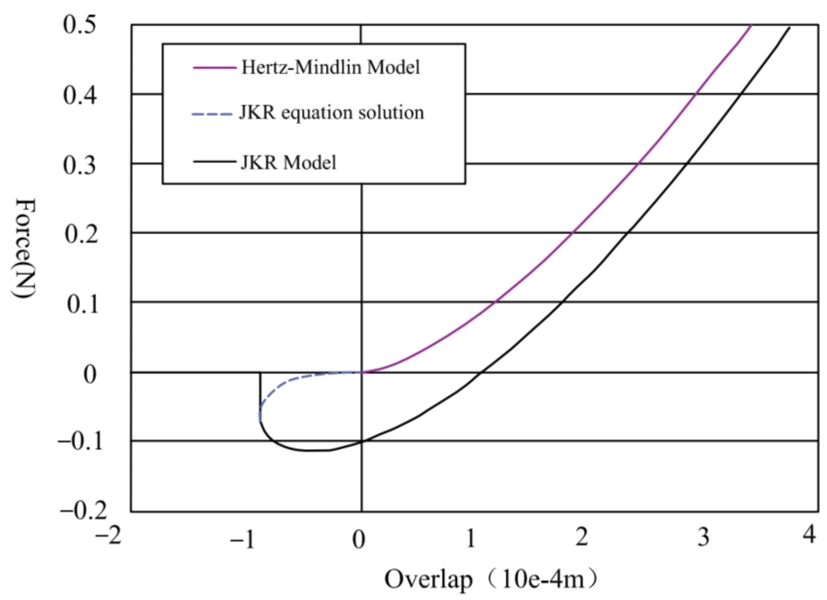
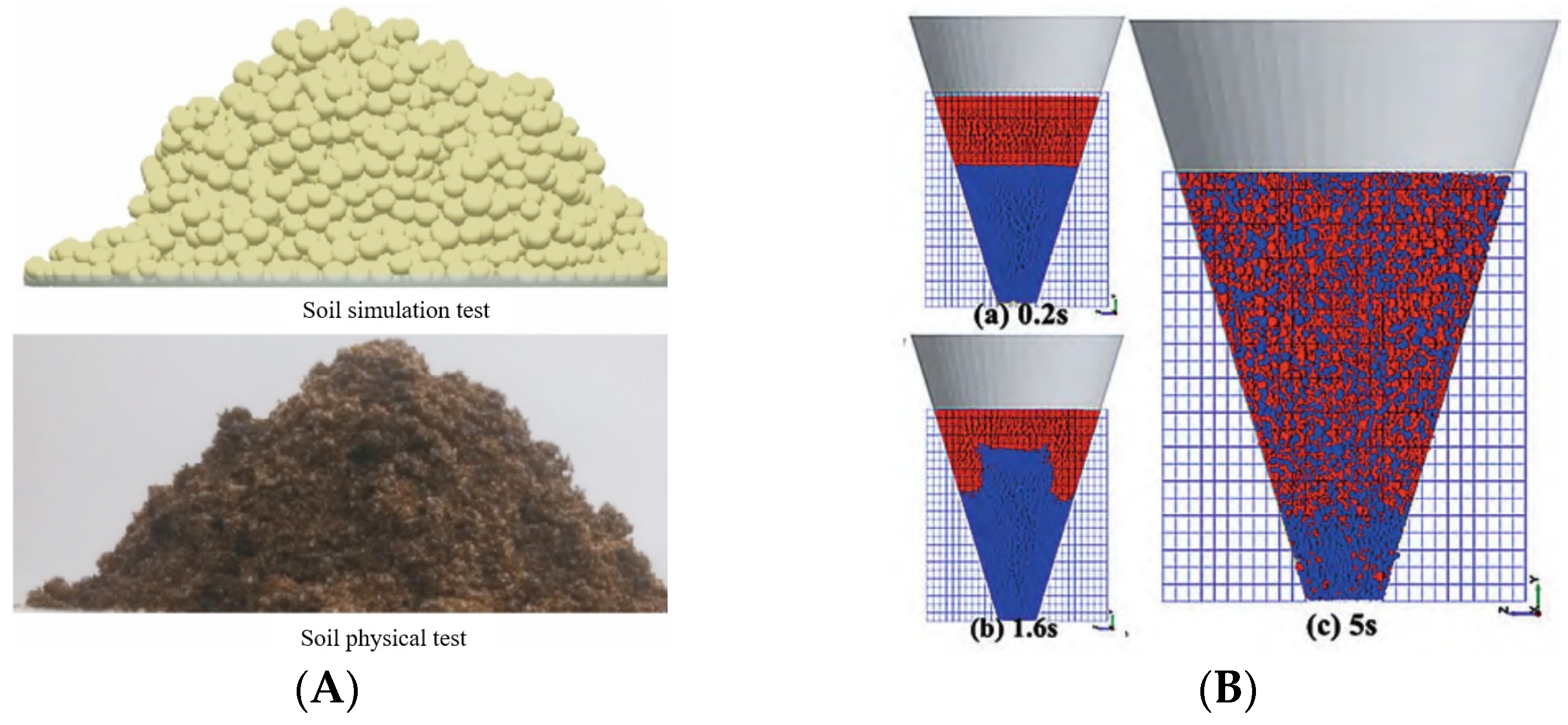
2.3. Hertz–Mindlin with JKR

The Hertz–Mindlin with the JKR contact model was proposed by Johnson in 1971 based on the Hertz model, taking into account the van der Waals forces, and it is a model that expresses the cohesion or adhesion between units by introducing an attractive force component that defines the attraction between the same and different discrete units and thus the cohesion or adhesion between the units [41] so that the JKR model can generate the surface adherence via the surface adhesion. Moreover, getting rid of the tension between discrete units requires additional mechanical energy to offset the surface energy adhesion, and then the disengagement distance between discrete units will be greater than the contact distance; the contact process is shown in Figure 5. At this time, the maximum gap δ_c and the maximum tensile force between discrete units F_pb is calculated as follows:

$${\delta }_c=\frac{{\alpha }_c^2}{R^{*}}-\sqrt{4\pi \gamma {\alpha }_c/E^{*}}$$

(11)

$${\alpha }_c={\left[\frac{9\pi \gamma R^{\ast 2}}{2E^{\ast }}\left(\frac{3}{4}-\frac{1}{\sqrt{2}}\right)\right]}^{1/3}$$

(12)

$$F_{pb}=-\frac{3}{2}\pi \gamma R^{\ast }$$

(13)

where ${\alpha }_c$ is the radius of the maximum discrete unit center spacing after detachment, $E^{\ast }$ is the modulus of elasticity, $R^{\ast }$ is the contact radius of the discrete unit, and $\gamma$ is the JKR surface energy.

Although the JKR model is proposed for smooth drying spheres, it can also act in the simulation of wet discrete units when the maximum adhesion tension $F_{pbw}$ after the contact detachment of the discrete units is related to the liquid surface tension ${\gamma }_s$ and the wetting angle $\theta$, which is calculated as follows:

$$F_{pbw}=-2\pi {\gamma }_{s}cos\left(\theta \right)\sqrt{R_1{R}_2}$$

(14)

The surface JKR energy of discrete units can be estimated by associating the wetting and drying maximum adhesion pull forces without scaling up the discrete unit model.

Subsequently, Johnson et al. also observed that the adhesion force is relatively insignificant under the discrete units subjected to higher loads in contact with each other. The overall characteristics exhibited are similar to those of the Hertz model, as shown in Figure 6 for the relationship between the discrete unit overlap and contact force for the Hertz–Mindlin contact model and the JKR contact model, which shows that with the gradual decrease in the load, the role of the adhesion force is gradually enhanced. The contact relationship of discrete units is also more and more important; when the amount of overlap is equal to zero, the Hertz–Mindlin contact model’s discrete units no longer produce force between them, while the JKR model also exists in the tensile force between the discrete units caused by the adhesion force, and the subsequent amount of overlap is negative to indicate that the two discrete units are separated from each other by a distance [42,43]. Therefore, the contact theory formulation of the JKR model is also similar to that of the Hertz–Mindlin (no-slip) model, which is divided into nonlinear adhesion forces in the standard and tangential directions and damping. But the JKR model simulates the cohesion and adhesion between discrete units through the definition of the attraction component; compared with the Hertz model, the JKR model can simulate the tension additionally brought about by the surface adhesion of the discrete units, as shown in Figure 5, in which discrete units will produce adhesion. The distance between the particles also needs to be more significant than the sum of the radii of the two particles in order for there to be detachment, and the Hertz model only has a more accurate simulation in the friction of the contact surface and does not produce mutual attraction when not in contact. The normal surface adhesion force F_JKR is shown in Equation (16) and is calculated consistently in both loaded and unloaded cases [41]:

$$\delta =\frac{{\alpha }^2}{R^{\ast }}-\sqrt{4\pi \gamma \alpha /E^{\ast }}$$

(15)

$$F_{JKR}=-4\sqrt{\pi \gamma E^{*}}{\alpha }^{\frac{3}{2}}+\frac{4E^{*}}{3R^{*}}{\alpha }^3$$

(16)

where $\alpha$ is the real-time discrete cell-contact radius.

When the surface JKR energy $\gamma =0$, the normal force formula agrees with Hertz–Mindlin (no-slip):

$$F_{HM}=\frac{4}{3}{E}^{\ast }\sqrt{R^{\ast }}{\delta }^{3/2}$$

(17)

Because of the existence of adhesion between discrete units of the JKR model, the adhesion that JKR can provide is only more pronounced between discrete units of small discrete units of the dust class [41]. The friction will be more significant than that of the Hertz–Mindlin (no-slip) model; initially, the JKR model was commonly used for the variations of the adhesion between discrete units that are a micrometer or smaller [44,45,46,47,48]. Gilabert and Baran [42,43] mentioned the modeling of discrete units of pulverized gravel and lunar soil using the JKR model. They found that the modified model can more accurately express the friction and rolling resistance between each of the two discrete units.

Therefore, the application of the JKR model in agricultural engineering is still focused on the modeling of materials with viscosity. Wu Tao and Xiang Wei [49,50] have used the JKR contact model to establish a discrete element simulation model of southern viscous soils. Xiang Wei followed up with a simulation and an actual comparison through the cavity molding test and found that the error of the two parameters of the opening longitudinal length and the adequate depth is less than 4%, which can more accurately express the contact characteristics of clay soil in southern China. Luo Shuai and Wang Liming [51,52] established a discrete element simulation model of livestock and poultry manure using the JKR model. They calibrated the parameters for swine manure with different moisture contents, and the errors of the contact characteristic tests were less than 10%, which was within a reasonable range. There are also the studies by Wang Weiwei, Huo Lili [53,54], etc., who used the JKR model for modeling the discrete unit of dust for biomass fuels and, through the hole mode compression of the simulation of the actual comparison test, found that the error is less than 2%, which is more accurate. Some application scenarios of the JKR model are shown in Figure 7.

A summary of the above literature applications shows that the JKR model is most accurately modeled for powdery discrete units that produce cohesion. This is also the closest to the application scenario for which the model was initially proposed. In the case of discrete units such as poultry manure and soil, where the particulate units are large and the utility of the surface JKR energy is poor, the accuracy of the simulated modeling force may be closer to the direct use of the Hertz–Mindlin (no-slip) model. In addition, soil manure initially has a certain water content. The theoretical derivation can also be seen in the water content of the JKR model of the maximum discrete unit’s detachment force, which also has a specific effect. Finally, simulation tests with large extrusion loads will also impact the accuracy of the JKR model. These are why it is challenging to simulate soils with specific firmness and water content during soil-modeling applications. Therefore, in agricultural engineering, the most suitable application scenario for the JKR model is still the simulation scenario of discrete powder units or as much reduction as possible in the simulated soil’s discrete unit size for simulation. This can better fit the JKR model’s computational theory prototype and reduce the model’s error.

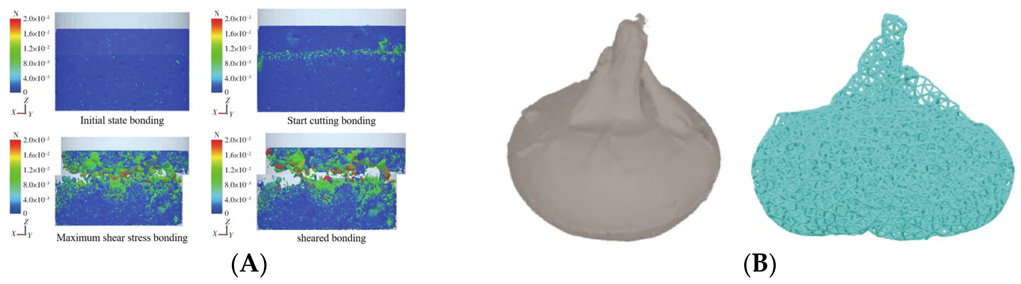
2.4. Hertz–Mindlin with Bonding Model

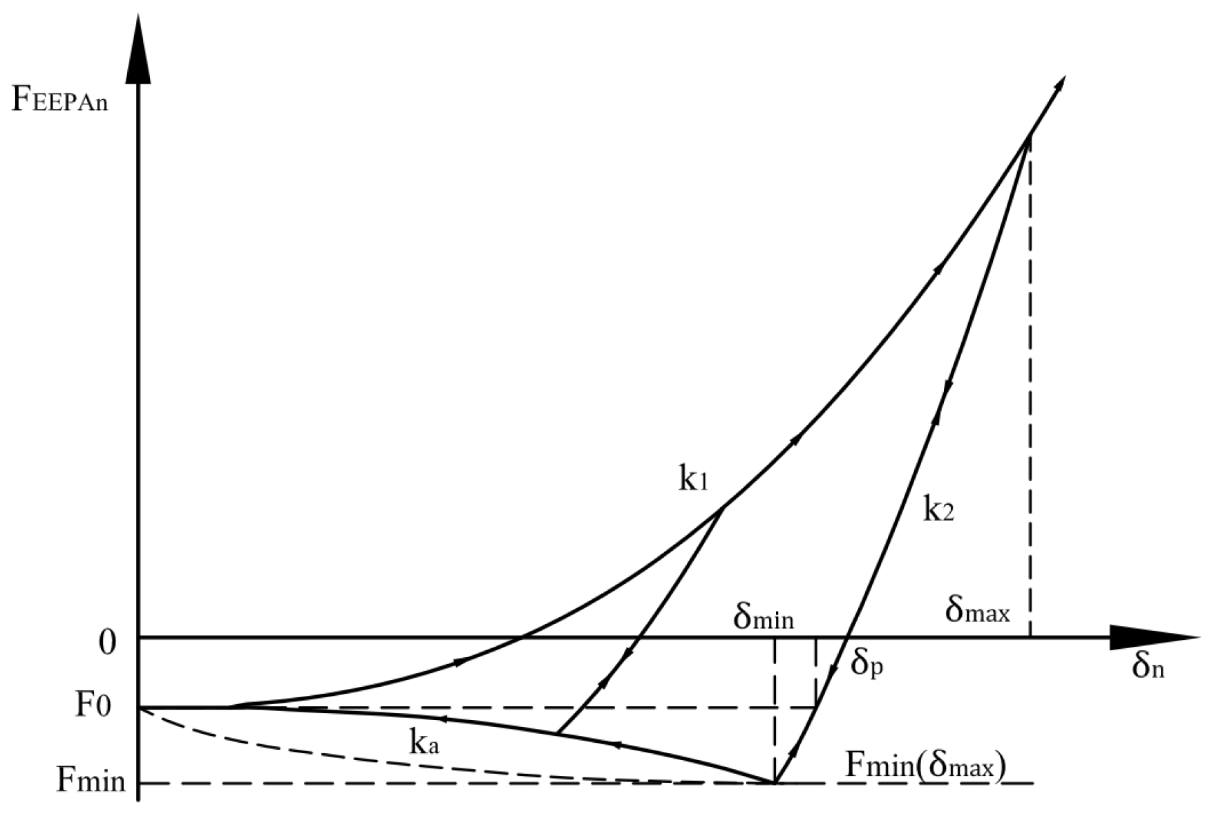
The bonding contact model is a new computational theory based on the Hertz–Mindlin model proposed by D.O. Potyondy and P.A. Cundall [55] in 2004. The model is used to observe the elasticity, fracture, and other properties of discrete rock units with non-uniform-sized spheres by stacking the bonding setup and the loading force. It is a very good model for characterizing rock simulation. The fracture process is characterized and widely used in this field [56,57,58,59].

When the bonding model is calculated in the contact force analysis, the force will be decomposed into the elastic force in the expected direction and the shear damping in the tangential direction. The bonding force between discrete units of the bonding model in the model is a fixed value formed during the initial loading process. The interactions between the discrete units before the bonding follow the Hertz–Mindlin (no-slip) contact model, and the bonding force between the discrete units is a fixed value formed during the initial loading process when the Bonding model of adhesion exists. The normal direction will exhibit a tensile force that prevents the discrete units from moving away from each other. This force is limited by the tensile strength of the discrete units themselves, while the tangential direction will exhibit shear damping that prevents the discrete units from slipping, which is limited by the shear strength. When the tensile force or the shear force in any direction exceeds the strength limit, the tangential tensile force and the tangential shear force generated by the bonding model will immediately disappear, at which point slipping will likely occur between tangential discrete cells. And subsequent discrete cell properties will be consistent with the linear model. The bonds will not form again even if subsequent squeezing occurs [60].

When the bonding model bonds during the action, the mechanical characteristics of the model and the linear model show a similar state. However, the bonding model of the linear and damping forces can be changed to the tensile state. The bonds during the action of the discrete units will not occur between the slipping, resulting in the damping force of the connecting bonds, which is also independent of the relative sliding state of the discrete units. Therefore, in the simulation process, when the bond between discrete units is formed, the tangential and normal forces and moments follow the bonding formula to be updated according to the time step. The specific formula is as follows [17]:

$$\delta F_N=-v_n{S}_{n}A{\delta }_t$$

(18)

$$\delta F_t=-v_t{S}_{t}A{\delta }_t$$

(19)

$$\delta M_N=-{\omega }_n{S}_{n}J{\delta }_t$$

(20)

$$\delta M_t=-{\omega }_t{S}_t\frac{J}{2}{\delta }_t$$

(21)

$$A=\pi R_B^2$$

(22)

$$J=\frac{1}{2}\pi R_B^4$$

(23)

where $F_{N,T}$ is the normal and tangential force of particle, $M_{N,T}$ is the normal and tangential torque of particle, $R_B$ is the bond radius, $S_{n,t}$ is the normal and tangential stiffness, ${\delta }_t$ is the time step, $v_{n,t}$ is the normal and tangential velocity of the discrete unit, and ${\omega }_{n,t}$ is the normal and tangential angular velocity of the discrete unit.

The bond will fracture when the force is updated to the usual tension limit or tangential shear limit, at which point the formula calculates the normal and tangential stress limits:

$${\sigma }_{max}<-\frac{F_n}{A}+\frac{2M_t}{J}{R}_B$$

(24)

$${\tau }_{max}<-\frac{F_t}{A}+\frac{M_n}{J}{R}_B$$

(25)

Like the bonds in the simulation application process in the generation, the discrete units that have not been in contact have been opened to show the force of mutual attraction. So the bonds in the application of parameter settings, as well as the contact radius, should be set slightly larger than the actual radius to simulate this process [17].

In agricultural engineering, the bonding model is also one of the widely used models; first of all, for applications in the soil field, Song Zhanhua [61] established a discrete element model of the soil of non-equal discrete units in a mulberry orchard, and through the simulation and the measurement of the actual straight shear internal friction angle error, found that the model’s error is 5.53%, which can be used for discrete element modeling of sandy soils. Hu Jianping [62] established a discrete element model of biaxial rotary plowing-straw-soil tillage for comparing models for the prediction of the power consumption of implements and found through the test that the error was 9.5%, and the model was representative. So bonding models are mainly used to observe bond breakage when applied to soils and are more widely used in modeling cohesive soils and clods. However, the comprehensive theory and application analysis is used to see the bonding model once the bonding bond fractures, the characteristics of the discrete units between the discrete units will follow the Linear model, and the soil characteristics have a large gap. But this model cannot be expressed on the soil cohesion or cohesion, only sandy soils, and the subsequent fracture model characteristics are closer to the rest of the soil type. If the remaining soil types need to be studied in the direction of soil fragmentation, they should refer to the research of Zhang Zhihong and Zhu Huibin [63,64]; the JKR and bonding models are used to jointly set up the soil contact calculations to ensure that there is still a JKR particle surface cohesion between the discrete units after the bonding bonds break to express the cohesion of the soil.

In addition, the bonding model is also widely used in the modeling of rhizomes and fruits, mainly in terms of two aspects. The first is for the small stalks of exudates or crushed stalks through the bonds to polymerize individual discrete units to simulate their shapes. According to Liao Yitao, CHAI X [65,66], used for the modeling of oilseed rape and rice crushed stalks, can be a better expression of the respective contact characteristics. The second aspect is the modeling of the soil-contact characteristics of the crushed stalks. Contact characteristics and the second aspect are the prediction of shear or extrusion destructive force on the overall stalks, fruits, and other parts through the setting of bond strength. Guo-Zhong ZHANG and Rui-Jie SHI [67,68] carried out discrete element simulation on the shear characteristics of water chestnut and caraway stalks, respectively, and the magnitude of the shear force was simulated better through the setting of bonds and the subsequent completion of the improvement in the tool or structure, which is of some reference significance. Some application scenarios of the bonding model are shown in Figure 8.

Although the bonding model was initially proposed for rock-fragmentation studies [55], it has been further extended to applications in the characterization of soil fragmentation, root crop cutting and fracture processes, and forces in agricultural engineering because of its ability to model connecting bonds that enable bonding and fracturing.

2.5. EEPA Model

The EEPA model is based on an extension of Walton’s Linear hysteretic model, which was developed by Morrisey in 2013 [69]. The EEPA model is similar to the rolling resistance linear model, which uses the exact mechanism of viscous damping superimposed on rolling resistance, allowing the elastic component to generate tension as well as a force–displacement relationship when in a nonlinear force–displacement relationship with respect to the compression. But the EEPA model also added additional viscous damping and resistance to rolling resistance, which can be observed through the cohesion and adhesion force changes between the same or different discrete units of the attractive force, and the model can also reflect when the discrete units are subjected to high loads of extrusion to produce plastic deformation resulting from increases in the contact area due to the increase in cohesion behavior. So the development of the initial stage model is mainly applied in the geotechnical compression test. Therefore, the model was initially developed for use in compression tests of soil mechanics to record the force variations of historical compression deformations. When applying the EEPA contact model for simulation calculations, similar to the linear model, the contact model is introduced for calculations only when the gap between the surfaces of the discrete units is detected to be less than or equal to 0 [17].

The updated formula for the contact force–displacement for the discrete cells within the time step of the EEPA model is shown in Equation [69]:

$$F_c=F_{EEPA}+F_d$$

(26)

$$M_c=M_r$$

(27)

where $F_c$ is the contact force, $F_{EEPA}$ is the nonlinear force, $F_d$ is the viscous damping force, $M_c$ is the contact moment, and $M_r$ is the rolling resistance moment.

In the process of simulation calculation, the nonlinear force is again decomposed into tangential and normal directions to be calculated separately, where the normal nonlinear force follows the average nonlinear force–displacement loading/unloading path model shown in Figure 5, where the horizontal coordinate is the length of the overlapping region of the discrete unit and the vertical coordinate is the value of the normal nonlinear force equal to the drag force (Figure 9).

When the contact between the discrete units just occurred (${\delta }_n=0$), the normal direction between the discrete units begins to produce a negative drag force $F_0$; at this time, with the overlap between the discrete units increasing, the initial loading change rule will follow the stiffness $k_1$ and overlap amount ${\delta }_n^m$ of the change curve. When the normal nonlinear force reaches the maximum, the model will record this time, the maximum amount of overlap ${\delta }_{max}$ unloading. The drag force follows the variation curve of the stiffness $k_2$ and the plastic overlap ${\delta }_p$. The power index (m) of the nonlinear curve in this stage is the same as that in the initial loading stage, and the stiffness coefficient $k_2$ is determined by the plastic strain ratio ${\lambda }_p$ of the simulation object following Equation (28):

$$k_2=\frac{k_1}{1-{\lambda }_p}$$

(28)

The stiffness $k_1$ is determined by the Young’s modulus of the simulated object, following Equation (29), which is similar in form to the Hertz model.

$$k_1=\frac{4}{3}{E}^{*}\sqrt{\overline{R}}$$

(29)

where $\overline{R}$ is

$$\overline{R}=\frac{R_1{R}_2}{R_1{+R}_2}$$

(30)

where $R_1$ and $R_2$ are the radii of the two mutually contacting discrete units.

The unloaded plastic overlap ${\delta }_p$, on the other hand, is related to the plastic strain ratio ${\lambda }_p$ and the power exponent (m) of the nonlinear curve, following Equation (31):

$${\delta }_p={\lambda }_p^{1/m}{\delta }_{max}$$

(31)

Between unloading overlap volumes, discrete cells generate a pulling force (adhesion force) on each other, which has a value equal to the drag force $F_0$, until the magnitude of the drag force reaches a minimum value ($F_{min}$), at which point

$$F_{min}=F_0-\frac{3}{2}\pi r^{*}$$

(32)

where r* is the adhesion energy assigned to the surface of the discrete unit in the JKR model, and a is the radius of the hypothetical plastic overlapping circular contact patch, which is derived from Equation (33) based on Hertz’s theory:

$$a=\sqrt{2{\delta }_p\overline{R}}$$

(33)

When the drag force reaches the minimum value $F_{min}$, the unloading stiffness coefficient will begin to follow the $k_a$ change curve, whose calculation formula is shown in Equation (34). At this time, the stage of the nonlinear curve of the power exponent (χ), the calculation needs to pay attention to keep the $k_a$ stiffness coefficient change curve the same as the $k_2$ stiffness coefficient change curve of the minimum value of the drag force $F_{min}$.

$$k_a=\frac{F_{min}-F_0}{{\delta }_{min}^{\chi }}$$

(34)

The formula for the amount of overlap at the minimum drag force is shown in the following equation:

$${\delta }_{min}={\left({\delta }_p^m+\frac{F_{min}-F_0}{k_2}\right)}^{1/m}$$

(35)

At this time, the stiffness coefficient $k_a$ is a variable that is affected by the minimum drag force $F_{min}$ of the loading and unloading histories and is determined by the unloading plastic overlap ${\delta }_p$ and the loading maximum overlap ${\delta }_{max}$.

From the above contact-calculation formula, it can be seen that the EEPA model, on the one hand, can be better applied in the simulation of soil discrete units and more accurately reflect the viscous and flow characteristics of soil discrete units in the field of agricultural engineering, mainly in the change in discrete unit flow in the ground soil after the operation of the machine tools, and the observation of the final shape and structure of the overall soil after the operation has been widely researched and applied. Wang Xianliang [70,71,72] established a discrete element discrete unit simulation model based on conservation tillage soil as a prototype through the tire–soil interaction simulation, and compaction soil deep-pine research validation found that the soil model can be used instead of the actual soil for simulation tests. Wanli Pengcheng [73,74,75] established a soil–trough soil-excavating plow discrete element simulation model, unfolded the discrete element simulation verification of harvesting components, and found that the simulation value and the actual error were within reasonable ranges. Dong Qianqian [76] analyzed the soil disturbance in each tillage layer during the vibratory deep-pine process through the simulation of cohesion and adhesion between discrete units of the EEPA model and observed the changing rules of the vibratory deep-pine trajectory and disturbance planes, as well as the transition zone, backfill zone, and disturbed zone under different operating speeds, and they verified the accuracy of the simulation model through field experiments. Yeon-Soo Kim [77] conducted a simulation of soil-tillage depth, soil-excavation plowing, and harvesting components through the model. They also simulated the tillage depth and traction force through the model and compared it with the actual test and found that the resistance error of the simulation was 7.5%, which was 5.3–61.6% more accurate than the theoretical prediction of the traction force. The accuracy was 20.3% higher than the single-layer soil model prediction considering the multi-layer soil characteristics.

Scholars have recently expanded the research on discrete units’ flow and adhesion characteristics based on the EEPA contact model. Subhash C [78] proposed a contact model for the quantitative prediction of the flow characteristics of cohesive powder based on the EEPA model and verified that it can be applied to limestone powder. Wenguang Nan [79] proposed a contact model based on the EEPA model for analyzing the flow characteristics between discrete units during a collision. Wenguang Nan [79] proposed a model based on the EEPA model to analyze the contact behavior between discrete units and the flow behavior of discrete unit agglomerates during a collision and found that the discrete calcium units have more robust adhesion characteristics than the EEPA model. However, the two models are not directly applicable in discrete element commercial software and still need further development. Some application scenarios of the EEPA model are shown in Figure 10.

The EEPA model, on the other hand, focuses on the ability to record the historical stress changes during the loading–unloading process of the model to record the correlation of stress changes during compression or shear. Fangping Xie [80] calibrated the discrete soil established by the EEPA model by conducting uniaxial confined compression and unconfined compressive strength tests on the soil. They obtained the optimal parameter combinations of the simulated soil after screening and compared the simulated values with the measured values, and they found that the EEPA modeled soil can accurately express the stress–strain behavior of the soil within the axial plastic deformation and the axial strain ranging from 3% to 45%. M. Javad Mohajeri [81] used a genetic-algorithm-calibration procedure to capture the different stress states of the discrete units of the EEPA model and the discrete unit history record correlation and corrected it. Then, the calibrated model’s parameters were verified through simulation with actual ring shear tests, which found that the model has a good correlation with the stress history data. Alvaro Janda [82] found an excellent stress-history data correlation of the EEPA model through the cone-penetration and unrestricted-compression tests to develop a study of the accuracy of the EEPA contact model for the simulation modeling of discrete elements of viscous solids, combined with simulation. Actual test comparisons found that the model can qualitatively reproduce the typical trends of the penetration-resistance curves in viscous discrete elements. Loading and deformation behaviors are independent of the size of the discrete elements used in the simulation process, and the contact model is more accurate.

The above article shows that EEPA can more accurately represent the changes in force and transport of discrete units with adhesion and flow characteristics. At the same time, the accuracy of applying stress–strain history records from the point of view of accuracy could be a lot better. However, this can be observed with the same trend as the actual situation, which is superior to the theoretical analysis of the results of the derivation of the existing discrete element commercial software contact model in the newer, more complex parameter setting. This is a model that is closer to the actual situation in the discrete element simulation of agricultural engineering soil.

The discrete element simulation model commonly used in agricultural engineering, as shown in

Table 1. Simulation parameters used in the discrete element method.

Contact Model	Model Type	Mechanical Behavior between Discrete Cells		Model Characteristics	Application Scenario
Linear	Linear elasticity Discrete cells are not deformable	Contact force = linear force + damping force Contact torque is always equal to zero		Discrete units in contact produce linearly varying compression and friction and do not resist the relative rotation of the units.	Geotechnics
HM (no-slip)	Nonlinear elasticity Discrete units can undergo small deformations	Contact force = Hertz nonlinear force + damping force Contact torque is always equal to zero		Discrete cells with small deformation variables produce nonlinear variations in squeezing and friction and do not resist relative rotation.	1. Discrete units for dryland soils 2. Crusty materials 3. Small discrete units of detritus
JKR	nonlinear elasticity	Contact force = JKR nonlinear force + damping force Contact moment = sliding resistance moment		JKR surface adsorption is significant at low pressures between small discrete cells, and adhesion will resist relative rotation.	1. Dust-like substances that generate mutual adsorption 2. Small discrete units of sticky material (soil, feces, etc.)
Bonding	Before bonding: nonlinear elasticity	Before bonding:	Consistent with HM model	Bonding bonds are generated before simulation and cannot be generated again once broken.	1. Sandy soils 2. Conformations of straw fruits and exudates and prediction of their shear–extrusion destructive forces
	Bonding: linear elasticity	When bonding:	Linear forces and damping can be stretched without slipping between discrete cells
	Fracture: linear elasticity	After the break:	Consistent with the linear model
EEPA	Nonlinear elasticity Plastic deformable	Contact force = EEPA nonlinear force + viscous damping force Contact moment = rolling resistance distance		1. Record of historical stress changes on discrete unit property changes after load application. 2. Discrete unit adhesion and flow.	1. Pre-loading of materials that affect discrete units 2. Observation of the flow characteristics of the discrete unit and the study of the final molding of the discrete unit under force

for the above model’s contact characteristics of the scene’s application, is summarized for the choice of the contact model to provide a specific theoretical basis and a new application direction.

3. Overview of Other Discrete Meta-Simulation Models in the Field of Agricultural Engineering

In addition to the models described above, several discrete element contact models in the field of agricultural engineering are similar to the models described above or are more specific to modeling soils, which are briefly described below.

3.1. Rolling Resistance Linear Model

The rolling resistance linear model is a contact calculation method similar to the linear model based on the research of Ai and Wensrich [83,84]. The contact torque is added based on the linear model to generate the rolling obstruction behavior. This torque increases linearly with the increase in the relative rotation of the contact point of the discrete unit, which is a better form of the rolling damping expression based on the linear model. However, the subsequent nonlinear model of the resistance to the rolling of the computational calculation of the theory of the simulation object is closer to the characteristics of the simulation object compared to the linear model, so the current application of this model in the field of agricultural engineering has been replaced by the nonlinear contact model, and the rolling resistance linear model is only applied in a few geotechnical research areas [85].

3.2. Adhesive Rolling Resistance Linear Model

The adhesive rolling resistance linear model, proposed by Gilabert [43] in 2007, is a linear contact model that expresses the attraction between discrete units, where the surrounding discrete units can be adsorbed through the setting of the attraction force and the attraction range, which is different from the van der Waals force of mutual attraction between tiny discrete units in the EEPA model. The adhesive rolling resistance linear model provides a linear fit of the van der Waals force between discrete units at short distances, and the model starts to work when the distance between discrete units is less than the attraction range [43,86]. Otherwise, the model does not work and is mainly used in the simulation of soil mixing. The properties of the materials in agricultural engineering are still the same as those of the EEPA model. The characteristics of materials in the field of agricultural engineering are still closer to the attractive adhesion setup of the EEPA model.

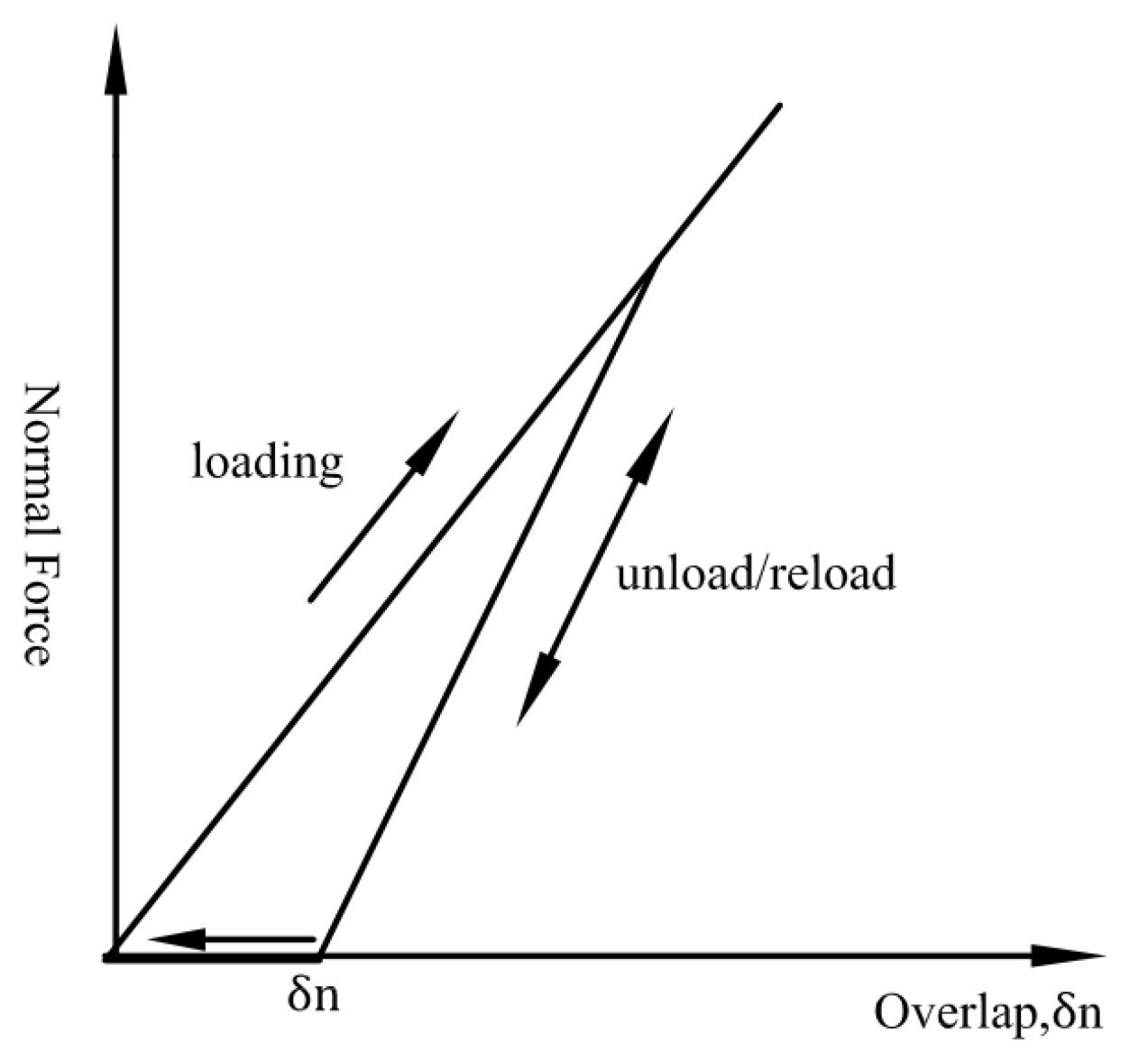
3.3. Hysteretic Model

The hysteretic model is a contact mechanics model proposed by Walton and Braun [87] in 1986 that allows discrete cells to deform plastically and is often considered an extended form of the linear spring model, where the elastic behavior between discrete cells is constrained by the setting of predetermined stress on the discrete cells. Once the contact stress is greater than the set stress, the discrete cells start to deform and their compression characteristics are simulated.

The relationship between the model contact force and the amount of overlap is shown in the curve in Figure 11. Unlike the EEPA model, the hysteretic model does not record the changes in the discrete units in the last loading and unloading cycle, so when the discrete units are separated, the discrete units will slowly become the same as those with the same stiffness and size before loading. It can be seen in the figure that when the amount of overlap is ${\delta }_0$, the contact force between the discrete units becomes 0. At this time, the amount of overlap is the remaining overlap between the recovery process of plastic deformation. When the remaining overlap amount becomes zero, the recovery of the discrete units is complete, and the contact characteristics and shape become consistent with the loading [87,88].

Based on their contact properties, hysteretic models are widely used to observe the performance of cyclic loading object properties [89,90,91], but there are fewer such cases in agricultural engineering, which do not have better application scenarios.

3.4. Other Models

In addition to the models mentioned above, there are also models with more fixed application scenarios, which are mainly still in rock–soil simulation. However, some of the properties may find new applications in the field of agricultural engineering in the future.

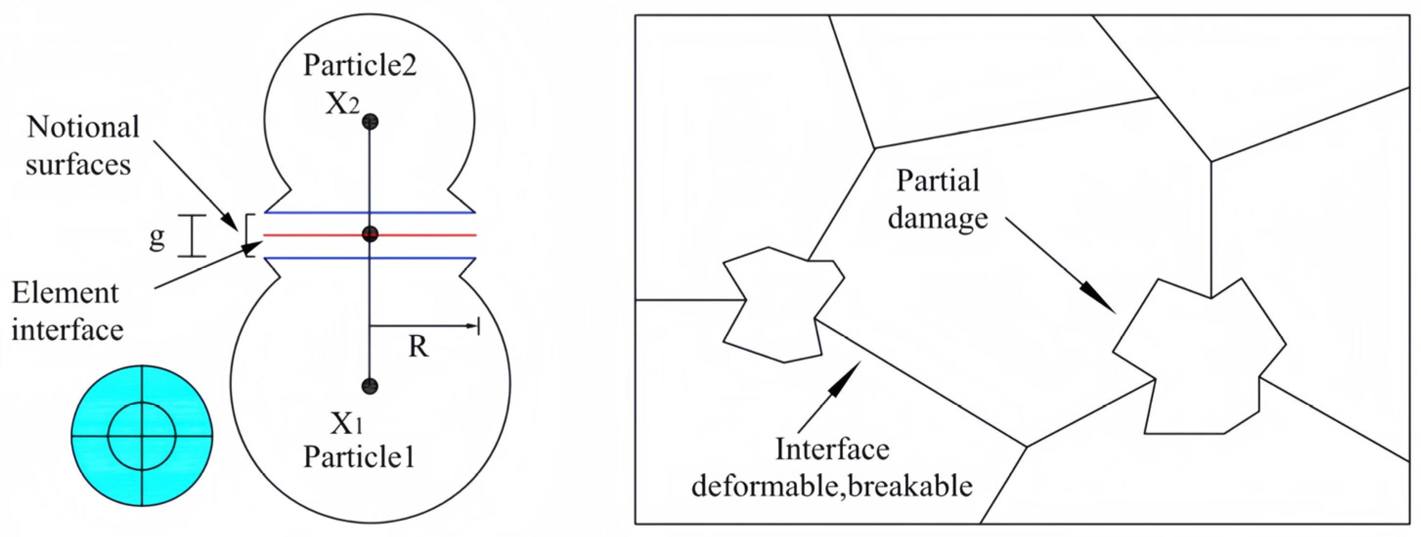
3.4.1. Flat-Joint Model

The flat-joint model is a contact-force-analysis theory proposed by Potyondy for models with flat joints and possible damage [92,93,94], and it is widely used in single flat contact and crystal discrete units in mutual contact. As shown in Figure 12, when the model starts to act, the contact surfaces of each discrete unit are determined as being bonded or unbonded. If bonding occurs at the interface, the kinematic behavior between the discrete units exhibits a linear elastic law. However, when the force separating the discrete units exceeds the bond strength limit, the interface will fracture, and some damage will be caused at the bonded surface. Moreover, when there is no bond between the contact planes, the interface will exhibit elastic and frictional motion [95,96].

This model structure has been widely studied in rock plane fractures. However, in the field of agricultural engineering, the flat-joint model of discrete cell interfaces bonded to each other has yet to be innovatively applied in scenarios by researchers, which is worthy of in-depth study.

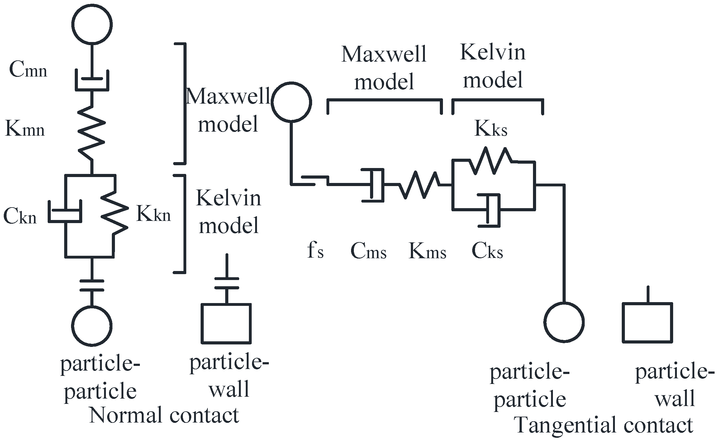
3.4.2. Burgers Model

The Burgers model is a commonly used contact model in soil rheological characterization that can more accurately characterize the elastic properties of soil flow. The model provides a Maxwell model, which acts in series in the standard and tangential directions, and a Kelvin model. The Kelvin model is a combination of linear springs and dampers, and the Maxwell model is a combination of linear springs and dampers that act in series, with a combination of a spring and a damper. The Burgers model acts on a tiny area and transmits only one force [97].

The Burgers model can better simulate the creep process of soil, as shown in Figure 13. When the load σ is applied to the soil, the elastic body, E₀ in the Maxwell model, immediately responds to the occurrence of the σ/E₀ strain. The deformation then occurs through the superposition of the motion of the damping body η₁ in the Maxwell model at the velocity σ/η₁ and the viscoelastic hysteresis motion of the Kelvin model. As t→∞, the Kelvin model deformation stops, and the curve gradually parallels the deformation curve of the η₁ damping body. This is a straight line of Newtonian flow, and the deformation will continue.

The model will resume the creep when the load is removed at some point t₁. First, the Maxwell model elastomer E₀ instantaneously recovers to its original length, and the Kelvin model will also recover fully as t→∞. However, the distance of the η₁ damping body flow cannot be recovered. The model then develops a residual deformation with a magnitude of σ_t1/η₁ (Figure 14).

From the analysis, it can be seen that the Burgers model can be a better representation of the creep characteristics of the soil, so it is also primarily used in this research area [98,99]; the applicable scene is narrower, and it is not easy to broaden the new application object.

It can be seen that there are still many models that have not been applied in the field of agricultural engineering and have not yet developed a good application scenario, as well as models where the model design is more specialized. In the future, in the simulation modeling of new agricultural work, objects can be used in the appropriate scenarios for innovative applications.

4. Trends in the Application of Contact Modeling for Discrete Element Simulation

With the continuous improvement in computer hardware and the deepening of contact analysis, it can be found that the development of contact models between discrete units has changed from the use of a single linear elasticity simulation to the incorporation of more and more properties into the simulation co-calculation, such as plastic deformation, adhesion, destruction, and the separation of discrete units, as well as the introduction of nonlinear forces, all of which imply more complex simulation and calculation rules per unit time step. However, advances in computer science mean that in the future, we can add more features to the development of contact models in order to simulate the simulation object more accurately. For example, the Nishihara model for siltstone [100] or the permafrost simulation model developed by Song Yungjun [101] with the addition of freezing load parameters have added additional parameters to their simulation objects, which are different from those of the original model, to supplement the characteristics that are not present in their models. The simulation results are also closer to reality and have reference significance. Therefore, referring to the summary of the above articles, the following predictions are made for the future development and application of the contact model.

(1)

From the analysis of the simulation model application, it can be seen that it is difficult to use a single model to simulate the operating objects in the field of agricultural engineering to thoroughly express all the characteristics of the material, and in the simulation and analysis of the mixture of materials in the process of the contact, the characteristics of the different substances are also different. Therefore, in the future, simulation should be used in combination with the multiple contact model of the discrete unit of the force and displacement for more accurate analysis and calculation. Therefore, the forces and displacements of discrete units should be analyzed and calculated more accurately in the future by mixing multiple contact models.

(2)

Many of the contact models used in agricultural engineering are based on the stress–strain calculation method and analyzed using geotechnical theory, and the contact characteristics in the simulation and analysis of crops differ significantly from the actual situation. Therefore, in the future, we need to design a particular contact model for the simulation object in the field of agriculture. By fitting the contact-fracture characteristics of the object through the setting of critical parameters such as spring, damping, slider, contact surface, and bonding key, the degree of similarity of the simulated object is fitted by the model and then assisted by the calibration process. According to the simulation parameters and application scenarios to be obtained on the simulation object, it needs to be determined whether it is a rigid body, whether it is plastic deformation, whether it is fracture damage, etc., for the establishment of a particular model so that the contact model of the force to match the deformation of the computational analysis of the actual situation as much as possible, to ensure the accuracy of the simulation model.

(3)

After determining the contact model, it is also necessary to determine and correct its physical or contact parameters through parameter calibration to ensure the accuracy of the model, and often, the error brought about by the measurement results at this time will also make the model show a big difference from the actual situation. Therefore, in the future, we should carry out a standardized process of physical and contact parameter determination for different contact models, find out the best determination method from the existing contact-parameter-determination method to unify the measurement specifications, and improve the accuracy of the discrete element method in the application of contact simulation in the field of agricultural engineering.

References

1. Zhang, X. Research on computer simulation technology and its application in agricultural engineering. China Rice 2021, 27, 150. [Google Scholar]
2. Chen, S.; Mao, H.; Jia, W. Computer Simulation Technology and Its Application in Agricultural Engineering; Jiangsu University Press: Zhenjiang, China, 2011. [Google Scholar]
3. Ma, Z.; Li, Y.; Xu, L. A review of discrete unit motion research in agricultural engineering. J. Agric. Mach. 2013, 44, 22–29. [Google Scholar]
4. Yu, J.; Fu, H.; Li, H.; Shen, Y. Discrete element method and its application in the research and design of working parts of agricultural machinery. J. Agric. Eng. 2005, 21, 6. [Google Scholar]
5. Zeng, Z.W.; Ma, X.; Cao, X.L.; Li, Z.H.; Wang, X.C. Current status and outlook of the application of discrete element method in agricultural engineering research. J. Agric. Mach. 2021, 52, 1–20. [Google Scholar]
6. Clough, R.W. The finite element in plane stress analysis. Proc. Am. Soc. Civ. Eng. 1960, 23, 337–345. [Google Scholar]
7. Cundall, P.A. A computer model for simulating progressive, large-scale movements in rocksy block systems. In Proceedings of the International Symposium on Rock Mechanics, Nancy, France, 4–6 October 1971. [Google Scholar]
8. Cundall, P.A.; Strack, O. A discrete numerical model for granual assemblies. Geotechnique 1979, 29, 47–65. [Google Scholar] [CrossRef]
9. Li, L. Research status and prospect of discrete element method in agricultural engineering. Chin. J. Agric. Mech. Chem. 2015, 36, 345–348. [Google Scholar]
10. Wang, W.; Li, X. A review of discrete element method and its application in geotechnical engineering. Geotech. Eng. Technol. 2005, 19, 177–181. [Google Scholar]
11. Yu, J.; Fu, H. Digital design software based on discrete element method and its application in the research and design of working parts of agricultural machinery. In Proceedings of the Abstracts of the Chinese Mechanics Society Academic Conference 2009, Zhengzhou, China, 24–26 August 2009; p. 435. [Google Scholar]
12. He, Y.; Wu, M.; Xiang, W.; Yan, B.; Wang, J.; Bao, P. Progress in the application of discrete element method in agricultural engineering. China Agron. Bull. 2017, 33, 133–137. [Google Scholar]
13. Hansong, J.I.; Song, Q.; Gupta, M.K.; Cai, W.; Zhao, Y.; Liu, Z. Grain scale modelling and parameter calibration methods in crystal plasticity finite element researches: A short review. J. Adv. Manuf. Sci. Technol. 2021, 1, 2021005. [Google Scholar]
14. Fang, W.; Wang, X.; Han, D.; Chen, X. Review of material parameter calibration method. Agriculture 2022, 12, 706. [Google Scholar] [CrossRef]
15. Coetzee, C.J. Calibration of the discrete element method. Powder Technol. 2017, 310, 104–142. [Google Scholar] [CrossRef]
16. Coetzee, C.J.; Scheffler, O.C. The Calibration of DEM Parameters for the Bulk Modelling of Cohesive Materials. Processes 2022, 11, 5. [Google Scholar] [CrossRef]
17. Itasca. PFC3D User Manual; Itasca Consulting Group Inc.: Minneapolis, MN, USA, 2003. [Google Scholar]
18. Hertz, H. Uber die beruhrung fester elastischer korper (On the contact of elastic solids). J. Reine Angew. Math. 1882, 91, 156–171. [Google Scholar] [CrossRef]
19. Mindlin, R.D.; Deresiewicz, H. Elastic Spheres in Contact Under Varying Oblique Forces. J. Appl. Mech. 1953, 20, 327–344. [Google Scholar] [CrossRef]
20. Tsuji, Y.; Tanaka, T.; Ishida, T. Lagrangian numerical simulation of plug flow of cohesionless particles in a horizontal pipe. Powder Technol. 1992, 71, 239–250. [Google Scholar] [CrossRef]
21. Elata, D.; Berryman, J.G. Contact force-displacement laws and the mechanical behavior of random packs of identical spheres. Mech. Mater. 1996, 24, 229–240. [Google Scholar] [CrossRef]
22. Ramírez, R.; Pöschel, T.; Brilliantov, N.V.; Schwager, T. Coefficient of restitution of colliding viscoelastic spheres. Phys. Review. E Stat. Phys. Plasmas Fluids Relat. Interdiscip. Top. 1999, 60, 4465–4472. [Google Scholar] [CrossRef] [PubMed]
23. Song, S.; Tang, Z.; Zheng, X.; Liu, J.; Meng, X.; Liang, Y. Calibration of discrete elemental parameters of a post-tillage soil model for cotton fields in Xinjiang. J. Agric. Eng. 2021, 37, 63–70. [Google Scholar]
24. Dai, F.; Song, X.; Zhao, W.; Zhang, F.; Navy, M.A.; Mingyi, M.A. Simulated calibration of discrete elemental contact parameters for full-film dihedral furrow mulching soil. J. Agric. Mach. 2019, 50, 49–56+77. [Google Scholar]
25. Zhang, R.; Han, T.L.; Ji, Q.L.; He, Y.; Li, J.Q. Research on the calibration method of sand and soil parameters in discrete element simulation. J. Agric. Mach. 2017, 48, 49–56. [Google Scholar]
26. Yan, D.X. Simulation Analysis and Experimental Research on Discrete Unit Modeling of Soybean Seed and the Process of Seed Casting, Mulching and Suppression. Ph.D. Thesis, Jilin University, Changchun, China, 2021. [Google Scholar]
27. Yan, D.; Yu, J.; Liang, L.; Wang, Y.; Liang, P. A Comparative Study on the Modelling of Soybean Particles Based on the Discrete Element Method. Processes 2021, 9, 286. [Google Scholar] [CrossRef]
28. Yan, L. A general modelling method for soybean seeds based on the discrete element method. Powder Technol. Int. J. Sci. Technol. Wet Dry Part. Syst. 2020, 372, 212–226. [Google Scholar] [CrossRef]
29. Song, X.-F.; Dai, F.; Shi, R.-J.; Wang, F.; Zhang, F.W.; Zhao, W.Y. Simulation and test of vibratory sorting of jute threshing material based on non-spherical discrete unit model. J. Agric. Eng. 2022, 38, 8. [Google Scholar]
30. Shu, C.; Yang, J.; Wan, X.; Yuan, J.C.; Liao, Y.T.; Liao, Q.X. Calibration and test of discrete element simulation parameters for combined harvesting of oilseed rape rejects. J. Agric. Eng. 2022, 38, 34–43. [Google Scholar]
31. Adajar, J.B.; Alfaro, M.; Chen, Y.; Zeng, Z. Calibration of discrete element parameters of crop residues and their interfaces with soil. Comput. Electron. Agric. 2021, 188, 106349. [Google Scholar] [CrossRef]
32. Liang, R.; Chen, X.; Zhang, B.; Wang, X.; Kan, Z.; Meng, H. Calibration and test of the contact parameters for chopped cotton stems based on discrete element method. Int. J. Agric. Biol. Eng. 2022, 15, 9. [Google Scholar] [CrossRef]
33. Liao, Y.; Wang, Z.; Liao, Q.; Wan, X.; Zhou, Y.; Liang, F. Parameter calibration of discrete elemental contact model for fodder rape stalks at early fruit pod stage. J. Agric. Mach. 2020, 51, 8. [Google Scholar]
34. Yu, Q.; Liu, Y.; Chen, X.; Sun, K.; Lai, Q.H. Calibration and test of simulation parameters of panax pseudoginseng seeds based on discrete elements. J. Agric. Mach. 2020, 51, 10. [Google Scholar]
35. Zhou, D. A study on the modelling method of maize-seed particles based on the discrete element method. Powder Technol. Int. J. Sci. Technol. Wet Dry Part. Syst. 2020, 374, 353–376. [Google Scholar] [CrossRef]
36. Wu, Q.; Liu, B.; Wang, Z.; Cai, Y. Numerical simulation and experimental study on stacking angle of lignite discrete units. Fertil. Des. 2021, 59, 5–8. [Google Scholar]
37. Wang, L.; He, X.; Hu, C.; Guo, W.S.; Wang, X.F.; Xing, J.F.; Hou, S.L. Determination of physical properties of coated cotton seeds and calibration of discrete element simulation parameters. J. China Agric. Univ. 2022, 27, 12. [Google Scholar]
38. Liu, F.Y.; Zhang, J.; Li, B. Discrete element parameter analysis and calibration of wheat based on stacking test. J. Agric. Eng. 2016, 32, 7. [Google Scholar]
39. Liu, C.; Wang, Y.; Song, J.; Li, Y.; Ma, T. Discrete elemental modeling and test of rice seeds based on three-dimensional laser scanning. J. Agric. Eng. 2016, 32, 7. [Google Scholar]
40. Aori, G.L.; Zhang, W.; Wang, S.; Liu, W.H.; Yu, Z.H. Determination of physical contact parameters of sunflower seeds with discrete element simulation calibration. Agric. Mech. Res. 2023, 45, 9. [Google Scholar]
41. Johnson, K.L.; Kendall, K.; Roberts, A.D. Surface Energy and the Contact of Elastic Solids. Proc. R. Soc. A Math. Phys. Eng. Sci. 1971, 324, 301–313. [Google Scholar]
42. Baran, O.; DeGennaro, A.; Rame, E.; Wilkinson, A. DEM Simulation of a Schulze Ring Shear Tester. In Proceedings of the 6th International Conference on Micromechanics of Granular Media, Golden, CO, USA, 13–17 July 2009; pp. 409–412. [Google Scholar]
43. Gilabert, F.A.; Roux, J.-N.; Castellanos, A. Computer simulation of model cohesive powders: Influence of assembling procedure and contact laws on low consolidation states. Phys. Rev. E 2007, 75, 011303. [Google Scholar] [CrossRef]
44. Antony, S.J.; Moreno-Atanasio, R.; Musadaidzwa, J.; Williams, R.A. Impact Fracture of Composite and Homogeneous Nanoagglomerates. J. Nanomater. 2008, 2008, 125386. [Google Scholar] [CrossRef]
45. Carrillo, J.M.Y.; Raphael, E.; Dobrynin, A.V. Adhesion of nanoparticles. Langmuir ACS J. Surf. Colloids 2010, 26, 12973–12979. [Google Scholar] [CrossRef] [PubMed]
46. Hassanpour, A.; Antony, S.J.; Ghadiri, M. Influence of interface energy of primary particles on the deformation and breakage behaviour of agglomerates sheared in a powder bed. Chem. Eng. Sci. 2008, 63, 5593–5599. [Google Scholar] [CrossRef]
47. Modenese, C.; Utili, S.; Houlsby, G.T. A Study of the Influence of Surface Energy on the Mechanical Properties of Lunar Soil Using DEM. In Discrete Element Modelling of Particulate Media; Wu, C.Y., Ed.; Chapter 9; RSC Publishing: Washington, DC, USA, 2012; pp. 69–75. ISBN 9781849735032. [Google Scholar]
48. Moreno-Atanasio, R.; Antony, S.J.; Ghadiri, M. Analysis of flowability of cohesive powders using Distinct Element Method. Powder Technol. 2005, 158, 51–57. [Google Scholar] [CrossRef]
49. Wu, T.; Huang, W.; Chen, X.; Ma, X.; Han, Z.Q.; Pan, T. Parameter calibration of a discrete element model for cohesive soil considering the bonding force between discrete units. J. South China Agric. Univ. 2017, 38, 93–98. [Google Scholar]
50. Xian, W.; Wu, M.; Lu, J.; Quan, W.; Ma, L.; Liu, J.J. Calibration of simulated physical parameters of clay loam soil based on stacking test. J. Agric. Eng. 2019, 35, 116–123. [Google Scholar]
51. Wang, L.; Fan, S.; Cheng, H.; Meng, H.B.; Shen, Y.J.; Wang, J.; Zhou, H.B. Calibration of contact parameters of swine manure based on EDEM. J. Agric. Eng. 2020, 36, 95–102. [Google Scholar]
52. Luo, S.; Yuan, Q.; Shaban, G.; Yang, L.Y. Parameter calibration of earthworm manure substrate discrete element method based on JKR bonding model. J. Agric. Mach. 2018, 49, 343–350. [Google Scholar]
53. Wang, W.; Cai, D.; Xie, J.; Zhang, C.; Liu, L.; Chen, L. Parameter calibration of discrete element model for dense molding of corn stover powder. J. Agric. Mach. 2021, 52, 127–134. [Google Scholar]
54. Huo, L.; Zhao, L.; Tian, Y.; Yao, Z.L.; Meng, H.B. Viscoelastic intrinsic model for biomass discrete unit fuel molding. J. Agric. Eng. 2013, 29, 200–206. [Google Scholar]
55. Dop, A.; Pac, B. A bonded-particle model for rock. Int. J. Rock Mech. Min. Sci. 2004, 41, 1329–1364. [Google Scholar]
56. Potyondy, D.O. The bonded-particle model as a tool for rock mechanics research and application: Current trends and future directions. Geosystem Eng. 2015, 18, 1–28. [Google Scholar] [CrossRef]
57. Obermayr, M.; Dressler, K.; Vrettos, C.; Eberhard, P. A bonded-particle model for cemented sand. Comput. Geotech. 2013, 49, 299–313. [Google Scholar] [CrossRef]
58. Song, Z.; Konietzky, H.; Herbst, M. Bonded-particle model-based simulation of artificial rock subjected to cyclic loading. Acta Geotech. 2019, 14, 955–971. [Google Scholar] [CrossRef]
59. Potyondy, D.O. Simulating stress corrosion with a bonded-particle model for rock. Int. J. Rock Mech. Min. Sci. 2007, 44, 677–691. [Google Scholar] [CrossRef]
60. Yoon, J.S.; Jeon, S.; Zang, A.; Stephansson, O. Bonded particle model simulation of laboratory rock tests for granite using particle clumping and contact unbonding. In Proceedings of the 2nd International FLAC/DEM Symposium, Melbourne, VIC, Australia, 14–16 February 2011. [Google Scholar]
61. Song, Z.; Li, H.; Yan, Y.; Tian, F.Y.; Li, Y.D.; Li, F.D. Parameter calibration and test of discrete element simulation model for non-equal-size discrete unit of mulberry soil. J. Agric. Mach. 2022, 53, 21–33. [Google Scholar]
62. Hu, J.; Zhao, J.; Pan, H.; Liu, W.; Zhao, X. A discrete element-based power consumption prediction model for a two-axis rotary tiller. J. Agric. Mach. 2020, 51 (Suppl. S1), 16–23. [Google Scholar]
63. Zhu, H.; Wu, X.; Bai, L.; Qian, C.; Zhao, H.; Li, H. Development of a dual-axis stubble breaking no-tillage device for rice stubble land based on EDEM-ADAMS simulation. J. Agric. Eng. 2022, 38, 10–22. [Google Scholar]
64. Zhang, Z.; Zhao, L.; Lai, Q.; Tong, J. Analysis and test of operating mechanism of shovel-plate type rolling soil touching component based on DEM-MBD coupling. J. Agric. Eng. 2022, 38, 10–20. [Google Scholar]
65. Liao, Y.; Liao, Q.; Zhou, Y.; Wang, Z.T.; Jiang, Y.J.; Liang, F. Parameter calibration for discrete element simulation of stalk crushing for fodder rape harvesting at shoot stage. J. Agric. Mach. 2020, 51, 10. [Google Scholar]
66. Chai, X.; Zhou, Y.; Xu, L.Z.; Li, Y.; Li, Y.; Lv, L. Effect of guide strips on the distribution of threshed outputs and cleaning losses for a tangential-longitudinal flow rice combine harvester. Biosyst. Eng. 2020, 198, 228–230. [Google Scholar] [CrossRef]
67. Zhang, G.; Chen, L.; Liu, H.; Dong, Z.; Zhang, Q.; Liu, Y. Calibration and test of discrete element simulation parameters of water chestnut. J. Agric. Eng. 2022, 38, 10. [Google Scholar]
68. Shi, R.; Dai, F.; Zhao, W.; Zhang, F.; Shi, L.; Guo, J. Establishment of discrete element flexibility model and experimental validation of contact parameters of caraway stalk. J. Agric. Mach. 2022, 53, 146–155. [Google Scholar]
69. Morrissey, J.P. Discrete Element Modelling of Iron Ore Pellets to Include the Effects of Moisture and Fines. Ph.D. Thesis, University of Edinburgh, Edinburgh, Scotland, 2013. [Google Scholar]
70. Wang, X.L.; Hu, H.; Wang, Q.J.; Li, H.W.; He, J.; Chen, W.C. Calibration method of soil model parameters based on discrete elements. J. Agric. Mach. 2017, 48, 78–85. [Google Scholar]
71. Wang, X. Research on Soil Compaction Evaluation and Combined Shovel Loosening Technology for Agricultural Machinery Operation. Ph.D. Thesis, China Agricultural University, Beijing, China, 2018. [Google Scholar]
72. Wang, X.; Zhong, X.; Geng, Y.; Wei, Z.C.; Hu, J.; Geng, D.Y.; Zhang, X.C. Calibration of no-till soil parameters based on discrete element nonlinear elastic-plastic contact model. J. Agric. Eng. 2021, 37, 100–107. [Google Scholar]
73. Li, P.; Li, Y.; Su, C.; Zhao, H.; Dong, Q.; Song, J.; Wang, S. Simulation of soil tillage characteristics based on EEPA contact model and analysis of spherical influence of discrete units. J. China Agric. Univ. 2021, 26, 193–206. [Google Scholar]
74. Li, P.; Li, Y.; Zhao, H.; Xu, G.; Song, J.; Dong, Q.; Zhang, C.; Wang, S. Asymptotic throwing characteristics of single-pendulum shovel-grid harvesting device for root crops. J. Agric. Eng. 2021, 37, 9–21. [Google Scholar]
75. Li, P.; Li, Y.; Jin, J.; Song, J.; Dong, Q.; Wang, S. Characterization of driving torque of single pendulum shovel fence harvesting device for root and tuber crops. J. Agric. Mach. 2022, 53, 191–200+339. [Google Scholar]
76. Dong, Q.; Su, C.; Zheng, H.; Han, R.; Li, Y.; Wan, L.P.; Song, J.; Wang, S. Analysis of soil disturbance process of vibratory deep loosening based on DEM-MBD coupling algorithm. J. Agric. Eng. 2022, 38, 34–43. [Google Scholar]
77. Kim, Y.S.; Siddique, M.A.A.; Kim, W.S.; Kim, Y.J.; Lee, S.D.; Lee, D.K.; Lim, R.G. DEM simulation for draft force prediction of moldboard plow according to the tillage depth in cohesive soil. Comput. Electron. Agric. 2021, 189, 106368. [Google Scholar] [CrossRef]
78. Thakur, S.C.; Morrissey, J.P.; Sun, J.; Chen, J.F.; Ooi, J.Y. Micromechanical analysis of cohesive granular materials using the discrete element method with an adhesive elasto-plastic contact model. Granul. Matter 2014, 16, 383–400. [Google Scholar] [CrossRef]
79. Nan, W.; Wei, P.G.; Rahman, M.T. Elasto-plastic and adhesive contact: An improved linear model and its application. Powder Technol. Int. J. Sci. Technol. Wet Dry Part. Syst. 2022, 407, 117634. [Google Scholar] [CrossRef]
80. Xie, F.; Wu, Z.; Wang, X.; Liu, D.; Wu, B.; Zhang, Z. Calibration of soil discrete element parameters based on unconfined compressive strength test. J. Agric. Eng. 2020, 36, 39–47. [Google Scholar]
81. Mohajeri, M.J.; Do, H.Q.; Schott, D.L. DEM calibration of cohesive material in the ring shear test by applying a genetic algorithm framework. Adv. Powder Technol. 2020, 31, 1838–1850. [Google Scholar] [CrossRef]
82. Janda, A.; Ooi, J.Y. DEM modeling of cone penetration and unconfined compression in cohesive solids. Powder Technol. 2016, 293, 60–68. [Google Scholar] [CrossRef]
83. Ai, J.; Chen, J.F.; Rotter, J.M.; Ooi, J.Y. Assessment of Rolling Resistance Models in Discrete Element Simulations. Powder Technol. 2011, 206, 269–282. [Google Scholar] [CrossRef]
84. Wensrich, C.M.; Katterfeld, A. Rolling Friction as a Technique for Modelling Particle Shape in DEM. Powder Technol. 2012, 217, 409–417. [Google Scholar] [CrossRef]
85. Jiang, M.; Shen, Z.; Wang, J. A Novel Three-Dimensional Contact Model for Granulates Incorporating Rolling and Twisting Resistances. Comput. Geotech. 2015, 65, 147–163. [Google Scholar] [CrossRef]
86. Gilabert, F.A.; Roux, J.-N.; Castellanos, A. Computer Simulation of Model Cohesive Powders: Plastic Consolidation, Structural Changes and Elasticity under Isotropic Loads. Phys. Rev. E 2008, 78, 031305. [Google Scholar] [CrossRef]
87. Walton, O.R.; Braun, R.L. Viscosity, granular-temperature, and stress calculations for shearing assemblies of inelastic, frictional disks. J. Rheol. 1986, 30, 949–980. [Google Scholar] [CrossRef]
88. Walton, O.R. Numerical simulation of inclined chute flows of monodisperse, inelastic, frictional spheres. Mech. Mater. 1993, 16, 239–247. [Google Scholar] [CrossRef]
89. Zhang, P.; Ren, Q.; Lei, D. Hysteretic model for concrete under cyclic tension and tension-compression reversals. Eng. Struct. 2018, 163, 388–395. [Google Scholar] [CrossRef]
90. Ji, A.; Li, T.A.; Rm, A.; Qu, B. Development of a hysteretic model for steel members under cyclic axial loading. J. Build. Eng. 2022, 46, 103798. [Google Scholar]
91. Nip, A.; Gardner, L.; Elghazouli, A.Y. Ultimate behaviour of steel braces under cyclic loading. Proc. Inst. Civ. Eng.-Struct. Build. 2013, 166, 219–234. [Google Scholar] [CrossRef]
92. Potyondy, D. PFC3D Flat-Joint Contact Model (Version 1); Technical Memorandum ICG7234-L; Itasca Consulting Group, Inc.: Minneapolis, MN, USA, 2013. [Google Scholar]
93. Potyondy, D. PFC2D Flat-Joint Contact Model; Technical Memorandum ICG7138-L; Itasca Consulting Group, Inc.: Minneapolis, MN, USA, 2012. [Google Scholar]
94. Potyondy, D.O. A Flat-Jointed Bonded-Particle Material for Hard Rock; In Proceedings of the 46th U. S. Rock Mechanics/Geomechanics Symposium, Chicago, IL, USA, 24–27 June 2012. Paper ARMA 12-501. [Google Scholar]
95. Potyondy, D.O. Material-Modeling Support in PFC [fistPkg25]; Technical Memorandum ICG7766-L; Itasca Consulting Group, Inc.: Minneapolis, MN, USA, 2017. [Google Scholar]
96. Potyondy, D. Flat-Joint Contact Model [Version 1]; Technical Memorandum 5-8106:16TM47; Itasca Consulting Group, Inc.: Minneapolis, MN, USA, 2016. [Google Scholar]
97. Gucunski, N. Fundamentals of Continuum Mechanics of Soils 1991. Soil Sci. 1992, 154, 170. [Google Scholar] [CrossRef]
98. Carcione, J.M.; Helle, H.B.; Gangi, A.F. Theory of borehole stability when drilling through salt formations. Geophysics 2006, 71, F31–F47. [Google Scholar] [CrossRef]
99. Carcione, J.M.; Poletto, F. Seismic rheological model and reflection coefficients of the brittle–ductile transition. Pure Appl. Geophys. 2013, 170, 2021–2035. [Google Scholar] [CrossRef]
100. Sun, X.; Mu, C.; Jiang, M.; Zhang, Y.; Yang, L.; Guo, B. Creep test and theoretical study of sandstone with different water content based on improved Nishihara model. J. Rock Mech. Eng. 2021, 40, 2411–2420. [Google Scholar]
101. Song, Y.; Zhang, L.; Ren, J.; Chen, J.; Che, Y.; Yang, H.; Bi, R. Triaxial creep characteristics of red sandstone and its modeling under freeze-thaw environment. J. Geotech. Eng. 2021, 43, 841–849. [Google Scholar]
Figure 1. Linear contact model. (a) Schematic of linear model contact force. (b) Linear model analysis.
Agriculture 14 00238 g001
Figure 2. Hertz–Mindlin (no-slip) contact model.
Agriculture 14 00238 g002
Figure 3. Model application scenarios. (a) Song Shaolong using the Hertz–Mindlin (no-slip) model to simulate Post-tillage soil in cotton fields. (b) Dai Fei using the model to simulate mulched soil.
Agriculture 14 00238 g003
Figure 4. Hertz–Mindlin (no-slip) model-application scenarios. (A) Dongxu Yan using the Hertz–Mindlin (no-slip) model to simulate a soybean; (a,b) are for the process of modeling from actual soybeans to simulation. (B) Song Xuefeng using the model to simulate a sesame stem; (C) Wang Long using the model to simulate coated cotton seed.
Agriculture 14 00238 g004
Figure 5. Contact process of the JKR model.
Agriculture 14 00238 g005
Figure 6. Overlap–load relationship curve of the JKR model.
Agriculture 14 00238 g006
Figure 7. JKR model application scenarios. (A) Wu Tao using the JKR model to simulate clay; (B) He Ping using the JKR model to simulate plastic powder.
Agriculture 14 00238 g007
Figure 8. Bonding model application scenarios. (A) Song Zhanhua using the bonding model to simulate the shearing process of soil in a mulberry field (B) Guo-Zhong ZHANG using the bonding model to simulate water chestnut to simulate the shearing force.
Agriculture 14 00238 g008
Figure 9. Overlap–load relationship curve of the EEPA model.
Agriculture 14 00238 g009
Figure 10. Application scenarios of the EEPA model. (a) Dong Xiangqian using the EEPA model to simulate soil disturbance state; (b) Sun Jianfeng using the EEPA model to simulate the rotary plowing process; (c) Subhash C. Thakur using the EEPA model to record direct shear stress.
Agriculture 14 00238 g010
Figure 11. Overlap–load relationship curve of the hysteretic model.
Agriculture 14 00238 g011
Figure 12. Contact theory of the flat-joint model.
Agriculture 14 00238 g012
Figure 13. Contact theory of the Burgers model.
Agriculture 14 00238 g013
Figure 14. Stress change of the Burgers contact model.
Agriculture 14 00238 g014